Notional Defined Contribution Pension Systems in a
Stochastic Context: Design and Stability
Alan J. Auerbach
University of California, Berkeley and NBER and
Ronald Lee
University of California, Berkeley and NBER December 2006
This research was supported by the U.S. Social Security Administration through grant #10-P-98363-1-02 to the National Bureau of Economic Research as part of the SSA Retirement
Research Consortium. The findings and conclusions expressed are solely those of the authors and do not represent the views of SSA, any agency of the Federal Government, or the NBER. The authors gratefully acknowledge the excellent research assistance of Erin Metcalf and Anne Moore, the contributions of Carl Boe in the development of the stochastic forecasting model, comments from Ed Palmer, Jason Seligman, Ole Settergren (none of whom is responsible for any remaining errors), participants in the NBER summer institute, the 8th annual RRC conference, and the October, 2006 NBER Conference on Retirement Research and support from Berkeley’s NIA-funded Center for the Economics and Demography of Aging. The research funded here builds on basic research funded by NIA grant R37-AG11761.
Abstract
Around the world, Pay-As-You-Go (PAYGO) public pension programs face serious long-term fiscal problems due primarily to actual and projected population aging, and most appear unsustainable as currently structured. Some have proposed the replacement of such plans with systems of fully funded private or personal Defined Contribution (DC) accounts, but the difficulties of transition to funded systems have limited their implementation. Recently, a new variety of public pension program known as “Notional Defined Contribution” or “Non-financial Defined Contribution” (NDC) has been created, with the objectives of addressing the fiscal instability of traditional plans and mimicking the characteristics of funded DC plans while retaining PAYGO finance.
Using different versions of the system recently adopted in Sweden, calibrated to US demographic and economic parameters, we evaluate the success of the NDC approach in achieving fiscal stability in a stochastic context. (In a companion paper, we will consider other aspects of the performance of NDC plans in comparison to traditional PAYGO pensions.) We find that the basic NDC scheme is effective at preventing excessive debt accumulation, but does little to prevent significant asset accumulation along many trajectories and on average. With adjustment, however, the NDC approach can be made more stable.
Keywords: Social Security, Retirement, Deficits JEL nos. H55, J11
Alan J. Auerbach Ronald Lee
Department of Economics Department of Demography
University of California University of California
549 Evans Hall 2232 Piedmont Ave
Berkeley, CA 94720-3880 Berkeley, CA 94720-2120
Introduction
Around the world, Pay-As-You-Go (PAYGO) public pension programs are facing serious long-term fiscal problems due primarily to actual and projected population aging, and most appear unsustainable as currently structured. All strict PAYGO programs (i.e., those that do not incorporate sizable trust fund accumulations) can feasibly pay an implicit rate of return equal to the growth rate of GDP (labor force growth plus productivity growth) once they are mature and in steady state. This rate of return is typically lower than the rate of return that can be earned in the market, either through low-risk bonds or through investment in equities. The programs’ long-term fiscal problems relate to a misalignment between these low but feasible rates of return and promised rates of return that may once have been feasible but no longer are so. The
traditional plans are mostly defined benefit, and have been criticized for creating strong incentives for early retirement. More generally there is a concern that the taxes that finance these programs distort labor supply incentives throughout life. Many also believe that these plans undermine motivations to save, and, because they are themselves unfunded, thereby reduce overall capital accumulation and consequently lead to lower labor productivity and slower growth.
Recently, a new variety of public pension program known as “Notional Defined Contribution” or “Non-financial Defined Contribution” (NDC) has been created and implemented by Sweden, with first payments in 2001. A number of other countries have introduced or are planning to introduce NDC plans, including Italy, Poland, Latvia, Mongolia and the Kyrgyz Republic, and proposed new plans for France and Germany have NDC aspects (Legros, 2003; Holtzmann and Palmer, 2005).
NDC programs differ in detail, but the basic principle is that they mimic Defined Contribution plans without actually setting aside assets as such plans do. Under an NDC program, a notional capital account is maintained for each participant. Balances in this account earn a rate of return that is declared by the pension plan each year; and notional payments into this account are made over the entire life history to mirror actual taxes or contributions.
Together with the declared rate of return these notional contributions determine the value of the account at any point in time. After a designated age such as 62, a participant can choose to begin to draw benefits, which is done by using the account to purchase an annuity from the pension plan. The terms of the annuity will depend on mortality at the time the generation turns 65 (for example) and on a rate of return stipulated by the pension plan, which might be the same rate of return used in the pre-retirement accumulation phase.
NDC plans are seen as having many potential advantages over traditional PAYGO systems, but our focus in this paper is on just one of these potential advantages, stability. A plan of this sort appears structured to achieve a considerable degree of fiscal stability because the promised rates of return reflect the program’s underlying PAYGO nature, rather than being market-based, and the annuity structure should buffer the system from the costs of rising longevity. Further, in the event that it begins to go off the tracks, a braking mechanism can be incorporated which automatically modifies the rate of return, to help restore the plan to financial health. Given the political difficulties of making frequent changes in PAYGO pension programs, the attractiveness of an inherently stable system is clear.
In this paper, we use a stochastic macro model for forecasting and simulating Social Security finances to examine the behavior of NDC-type public pension programs in the context of the US demography and economy. Given the structure and strategy of the stochastic model,
we can study the probability distribution of outcomes (benefit flows and rates of return) for generations (birth cohorts) of plan participants for the NDC program, as well as the overall financial stability of the NDC system. The next section of the paper describes our stochastic forecasting model. In the following section, we describe in some detail the Swedish NDC program and our adaptation of it to US economic and demographic conditions. We then provide simulations of this basic US NDC plan, as well as variants incorporating modifications of two key attributes of the NDC plan, the method of determining rates of return, and the brake mechanism applied when the system appears headed for financial problems.
The Stochastic Forecasting/Simulation Model
The stochastic population model is based on a Lee-Carter (1992) mortality model and a somewhat similar fertility model (Lee, 1993; Lee and Tuljapurkar, 1994). Lee-Carter models the time series of a mortality index as a random walk with drift, estimated over US data from 1950 to 2003. This index then drives the evolution of age specific mortality rates and thereby survival and life expectancy. This kind of model has been extensively tested (Lee and Miller, 2003) and is widely accepted (Booth, 2006), and although we shall see that the probability intervals it
produces for distant future life expectancy appear quite narrow, these intervals have performed well in within-sample retrospective testing.
In a similar way, a fertility index drives age specific fertility, but in this case it is necessary to prespecify a long term mean based on external information. We set the long run mean of the Total Fertility Rate equal to the 1.95 births per woman, as assumed by the Social Security Actuaries (Trustees Report, 2004, henceforth TR04). The estimated model then supplies the probability distribution for simulated outcomes. Because it is fitted on US data, the fertility model reflects the possibility of substantial baby boom and bust type swings.
Immigration is taken as given and deterministic, following the assumed level in TR04. Following Lee and Tuljapurkar (1994), these stochastic processes can be used to generate stochastic population forecasts in which probability distributions can be derived for all quantities of interest. These stochastic population forecasts can be used as the core of stochastic forecasts of the finances of the Social Security system (Lee and Tuljapurkar, 1998a and b, and Lee, Tuljapurkar Anderson, 2003). Cross sectional age profiles of payroll tax payments and benefit receipts are estimated from administrative data. The tax profile is then shifted over time by a productivity growth factor which is itself modeled as a stochastic time series. The benefit age profile is shifted over time in more complicated ways based on the level of productivity at the time of retirement of each generation. The real rate of return on special issue Treasury Bonds is also modeled as a stochastic time series, and used to calculate the interest rate on the Trust Fund Balance. The long run mean values of the stochastic processes for productivity growth and rates of return are constrained to equal the central assumptions of TR04, but the actual stochastically generated outcomes will not exactly equal these central assumptions, of course, even when averaged over a 100 year horizon.
The probability distributions for the stochastic forecasts are constructed by using the frequency distributions for any variable of interest, or functions of variables of interest, from a large number of stochastically generated sample paths, say 1000, typically annually over a 100 year horizon. Essentially, this is a Monte Carlo procedure. The stochastic sample paths can equally well be viewed as stochastic simulations, and the set of sample paths can be viewed as describing the stochastic context within which any particular pension policy must operate.
The stochastic simulation model is not embedded in a macro-model, and therefore does not incorporate economic feedbacks, for example to saving rates and capital formation, and
hence to wage rates and interest rates. For some purposes, this would be an important limitation. However, the model has given useful results for the uncertainty of Social Security finances, and it should also give useful results in the present context. Once the stochastic properties of different policy regimes have been studied in this manner, it may be appropriate to extend the analysis to incorporate more general economic feedbacks in future work.
A Stochastic Laboratory: Simulating Statistical Equilibrium
To date, the stochastic Social Security method just described has been used solely for projections or forecasts, based on the actual demography and Social Security finances of the United States. However, it can also be used as a stochastic laboratory to study how different pension systems would perform in a stochastic context divorced from the particularities of the actual US historical context with its baby boom, baby bust and other features. This is the main strategy we pursue in this paper, since we are hoping to find quite general properties of the NDC systems. We build on the important earlier work by Alho et al. (2005). This approach also enables us to avoid dealing initially with the problems of the transition from our current system to the new system. Instead we will analyze the performance of a mature and established system in stochastic steady state. In later work we hope to consider the transition and to account for the actual historical initial conditions such as the current age distribution as shaped by the baby boom.
The key feature of a stochastic equilibrium is that the mean or expected values of fertility, mortality, immigration, productivity growth, and interest rates have no trend, and the population age distribution is stochastically stable rather than reflecting peculiarities of the initial
conditions. The basic idea is simple enough, but there are a number of points that require discussion, as follows.
1. Productivity growth and interest rates are already modeled as stationary stochastic processes with preset mean values, so these pose no particular problem.
2. Net immigration is set at a constant number per period, following the Social Security assumptions (TR04). We treat immigration as deterministic and constant.
3. Fertility is also modeled as a stationary stochastic process with a long-term mean value of 1.95 births per woman, consistent with TR04. This is below replacement level, so absent positive net immigration, the simulated population would decline toward zero and go extinct, with the only possible equilibrium population being zero. But with immigration, there is some population size at which the natural decrease given a TFR of 1.95 will be exactly offset by the net immigrant inflow, and this will be the equilibrium population. The same principle applies in a stochastic context.
4. According to the fitted Lee-Carter mortality model, the mortality level evolves as a random walk with drift. First, we note that unless the drift term is set to 0, mortality will have a trend. So in constructing our stochastic equilibrium population, we will project mortality forward, with drift, until 2100 and then set the drift to zero thereafter. This sets equilibrium life expectancy at birth to be about 87 years. Second, we note that a random walk, even with zero drift, is not a stationary process. It has no tendency to return to an equilibrium level, but rather drifts around. Our strategy is simply to set the drift term to zero. This means that we cannot view the simulated process as truly achieving a statistical equilibrium, but this is unlikely to cause any practical problems. An alternative would be to alter the model to make it truly stationary by providing some weak equilibrating tendency, e.g. replacing the
5. We also need to generate an appropriate initial state for our system. We begin by
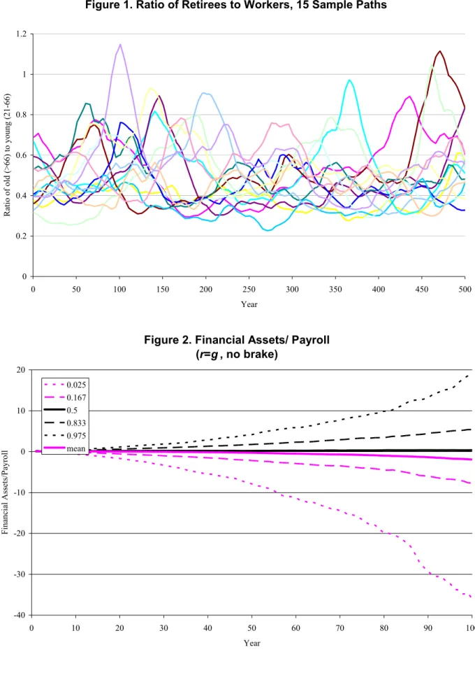
constructing a deterministic stable population corresponding to the mean values of fertility and mortality for the given inflow of immigrants. Population size adjusts until the net inflow of immigrants is equal to the shortfall in births due to below-replacement fertility. We then start our stochastic simulation from this initial population, but we throw out the first hundred years. We keep the next five hundred years of stochastic simulations as our experimental set. Figure 1 plots 15 stochastic sample paths for the old age dependency ratio defined as
population 67+ divided by the population 21 to 66. Evidently the simulations often show very pronounced long term variations resulting from something like the baby boom and baby bust in the United States.
6. For our policy experiments, we have created a single set of 1000 sample paths or stochastic trajectories. We will examine the performance of different policies within the context of this single set of stochastic trajectories, so that each must deal with the same set of random shocks, which makes their performances more comparable.
NDC System Design
As is well-known, the feasible internal rate of return for a PAYGO system with stable population structure equals the rate of growth of the population (which equals the rate of growth of the labor force, in steady state) plus the rate of growth of output per worker. Alternatively, this implicit rate of return simply equals the growth rate of GDP, provided that covered wages are a constant share of GDP. NDC systems aim to mimic the structure of funded DC systems while maintaining fiscal stability by using such an internally consistent rate of return (with due allowance for the non-steady state context) rather than a market-based rate of return.
As under any pension system, an individual goes through two phases under an NDC scheme, corresponding roughly to periods of work and retirement. During the work phase, the individual’s payroll taxes (T) are credited to a virtual account typically referred to as the
individual’s “notional pension wealth” (NPW). Like the individual account under an actual DC plan, this account has a stated value that grows annually with contributions and the rate of return on prior balances; for an individual, this evolution is represented by:
(1) i t t t t NPW r T NPW+1 = (1+ )+ where i t
r is the rate of return credited to each individual’s existing balances. Unlike the individual account balance under the DC plan, NPW is only a virtual balance and the rate of return is based on the system’s internal growth rate. Once an individual retires, he or she receives an annuity based on the value of notional pension wealth at the time of retirement.
The Swedish system normally bases ri on the contemporaneous rate of growth of the wages per worker, which we call g, rather than the total growth of wages, which would also account for the growth rate of the work force, which we label n.1 The notional accounts of individuals in Sweden also receive an annual adjustment for so-called inheritance gains, representing a redistribution of the account balances of deceased cohort members. That is, the rate of return to the cohort as a whole, which we denote r, equals g, where r=g<ri.2
Upon retirement in the Swedish system, the individual’s NPW is converted into an annuity stream based on contemporaneous mortality probabilities and an assumed real rate of
1 Our characterization of the Swedish system relies on several sources, including Palmer (2000) and Settergren
(2001a, 2001b).
2 Accounts in Sweden are also reduced annually to account for administrative costs. In our simulations, we ignore
return of 1.6 percent. Letting the superscript t denote the generation that reaches retirement age in year t, the annuity in year t for an individual retiring that year, t
t
x , may be solved for implicitly from the formula,
(2) ( 1) ( 1) , , (1.016) (1.016) T T t s t t t t s t t t t s t t t s s t s t NPW − − + P x x − − + P = = =
∑
=∑
where t tNPW is the individual’s notional pension wealth in the year of conversion, t s t
P, is the probability of survival from year t until year s, assessed in year t, and T is the maximum life span. In subsequent years, the individual’s annuity level is increased or decreased according to whether the actual average growth of wages per worker, denoted rt = gt above, exceeds or falls
short of 1.6 percent. If wage growth continues at 1.6 percent then the annuity level would
remain constant in real terms throughout the individual’s life. However, if the realized growth of wages per worker in year t were actually 1.3 percent, the annuity would be 0.3 percent lower in real terms in year t+1 than in year t. If r were 1.3 percent in every year, the annuity would fall in real terms at a rate of 0.3 percent per year.
The Brake Mechanism
The system just described incorporates an adjustment mechanism aimed at keeping benefits in a range that can be supported by growth in the payroll tax base. However, the adjustment is not perfect. First, although benefits are adjusted annually for changes wage growth, they are not adjusted after retirement to reflect changes in mortality projections. More importantly, the cohort rate of return r in the Swedish system is based on the growth rate of the average wage, g. While this approach might be more comprehensible from an individual
payroll, n+g, would automatically take into account another determinant of the system’s capacity to provide benefits, the growth rate of the work force Finally, as illustrated in the Appendix using a simplified version of the NDC plan, even an NDC plan without these problems is not assured of annual balance if n+g varies over time. This is in line with the analysis of Valdes-Prieto (2000), who observed that, under certain conditions, an NDC plan might be stable in a steady state, but will not be so in the short run.
Although it was anticipated by its designers that the Swedish system would nevertheless be quite stable, they added to the system a balance mechanism3, which we call a “brake,” that would slow the growth rate of notional pension wealth and reduce the level of pension benefits in the event of a threat to the system’s financial stability, as measured by a “balance ratio” b based on the system’s conditions,
(3) P NPW C F b + + =
The numerator of the balance ratio is meant to account for the system’s assets, and is the sum of two terms. The first term in the numerator (F) equals the financial assets of the system (negative if the system has financial debt); the second term in the numerator (C) is a so-called “contribution asset” equal to the product of a three-year moving median of tax revenues and a three-year moving average of “turnover duration,” which is the average expected length of time between the payment of contributions and the payment of benefits, based on current patterns. If the economy were in a steady state, the contribution asset would provide a measure of the size of the pension liability that contributions could sustain.
The denominator is the pension system’s liability, equal to the sum of two components. The first component of the denominator (NPW) is aggregate notional pension wealth for
generations not yet retired; the second component (P) is an approximation of commitments to current retirees, equal to the sum over retired cohorts of current annual payments to each cohort multiplied by that cohort’s so-called economic annuity divisor, roughly the present value of their annuities calculated using the assumed 1.6 percent real return.4
This balance measure can be calculated entirely from observed values and does not involve any projected values. This has the advantage of reducing the risk of political
manipulation, but a disadvantage in not taking advantage of all information available at the time in computing the contribution asset and the liability to current retirees, basing them simply on current conditions.
The balance ratio is not a perfect measure of the system’s financial health. For example, the two components of the asset measure are based on inconsistent rate-of-return assumptions, the financial component being assumed to yield a market rate of return and the contribution asset being valued using the system’s implicit rate of return. However, one would still expect a higher value of the balance ratio, in general, to be associated with a more viable system.
We refer to the Swedish balance mechanism as a “brake” because its effect is to prevent the excessive accumulation of debt, but not of assets; it applies only when the system is
underfunded, as indicated by the balance ratio, but not when it is overfunded. It was understood when the system was designed that this potentially could lead to the accumulation of surpluses, but no formal mechanism was put in place to deal with this. One could imagine a system with a
more symmetric brake that raises benefits and pension accumulations when the system is overfunded, and we consider such a system below.
For the Swedish system, the balance mechanism is activated only when the balance ratio
b falls below 1.0, and stays in effect until a test of fiscal balance is satisfied. While the
mechanism is active, two things happen each year. First, cohort pension wealth accumulates not at a gross rate equal to (1+gt), but instead at a rate equal to (1+gt)bt, where bt is the balance ratio.
Second, the gross rate of growth used to adjust the pension benefits of retirees is also set equal to (1+gt)bt, meaning a greater likelihood of a real decline in pension benefits for any given cohort,
since real benefits grow at a gross rate of (1+gt)bt/ 1.016. The balance mechanism remains in
effect as long as the product of balance ratios from each year of the episode remains below 1.0. That is, if the balance ratio first falls below 1.0 in year t, then the balance mechanism continues to apply in year s>t if
∏
<1.0=
s
t v v
b . Once this product exceeds 1.0, the balance mechanism is taken off, with a new episode beginning the next time the balance ratio again falls below 1.0.
This design has several implications. First, because the balance mechanism is removed when the product of balance ratios first moves above 1.0, the balance ratio must exceed 1.0 in the year the balance ratio is removed. Second, as the balance ratio may stay below 1.0 for some time, there may be several years during the episode for which b > 1.0. Third, as mentioned above, the balance mechanism is asymmetric, in that it applies only when b first falls below 1.0; paths on which b starts above 1.0 and rises well above this level are subject to no external adjustment. Fourth, there may be recurrent episodes during which the balance mechanism is in effect. Fifth, while the balance ratio as defined in (3) can be negative (if financial debt exceeds the contribution asset), the balance mechanism is not meaningful for b < 0, for this would call for more than complete confiscation of pension wealth and benefits.
As to the logic of the test imposed to determine when the balance mechanism is removed, based on the product of balance ratios, this approach ensures that the balance mechanism has no long-run impact on the level of benefits. That is, the cumulative gross rate of return from the first year in which the brake applies, say t, through the year, say T, in which the product of the balance ratios reaches 1.0 and hence the brake mechanism is removed, is
(1+gt)bt*(1+gt+1)bt+1*…*(1+gT)*bT = (1+gt)*… *(1+gT)*(bt*… * bT) = (1+gt)*… *(1+gT).
Even though there is no impact on the long-run level of benefits, the brake mechanism has the capacity to reduce debt accumulation by keeping benefits below their regular long-run path for some time.
Adapting the NDC System to the US Context
We have already outlined the basic structure of the Swedish NDC system, but there are various details to be specified in adapting the system to the US context.
Contributions
What proportion of payroll is to be contributed? For comparability to our current Social Security system, we assume the OASI tax rate of 10.6 percent, applied to the fraction of total wages below the payroll tax earnings cap.
Rates of Return
Rate of return assumptions are required in two places in the NDC system, for use in accretions of Notional Pension Wealth and in conversion of Notional Pension Wealth into an annuity stream upon retirement. The Swedish plan sets the first of these rates equal to the growth rate of average wages, which should roughly equal the growth rate of productivity. It sets the second rate equal to 1.6 percent, taken to be the expected rate of productivity growth, and then adjusts annuities up or down in response to variations in the actual growth of the
average wage. Sweden does not account for the growth rate of the labor force but in principle it should be included since it is a component of the rate of return to a PAYGO system. Note that even if the growth rate of the labor force is not included, demography will still influence the outcomes for generations through the back door, because if the system begins to go out of fiscal balance then the brake will be applied.
For the US system, we take the long-run mean rate of growth of the real covered wage to be 1.1 percent, following the Social Security assumption (TR04), as described below. We will refer to this interchangeably as the productivity growth rate or the growth rate of wages, g, although these are actually somewhat different concepts.5 We have implemented NDC in two ways for the United States, once with rate of return based only on wage growth (g), and once with the rate of return based on both wage growth and labor force growth (n+g). These will presumably distribute risk in different ways across the generations. In stochastic equilibrium population growth is near zero in any case, on average, but demographic change will certainly occur along simulated sample paths.
Annuity Calculations
We assume that annuitization of NPW occurs at age 67, the normal retirement age to which the US system is currently in transition. We use the same rate of return for accumulations of NPW as in converting the account balance at retirement into an annuity stream. That is, we use either the growth rate of wages (g) or the growth rate of wages plus labor force (n+g) in both cases. As in the Swedish system, we set the pattern of the annuity stream to be constant in real
5We note that the growth rate of productivity (output per hour of labor) may overstate the growth rate of covered wages, as is explicitly taken into account by the US Social Security Administration. The growth rate of covered wages will be affected by changes in the supply of labor per member of the population of working age and by sex, both labor force participation and hours worked per participant, and by shifts in the population age distribution. It will also be affected by the proportion of compensation that is given in pretax fringe benefits.
terms, based on the growth rate and mortality projections at the time of the original annuity computation. Unlike the Swedish system, we use the actual growth rate (either g or n+g) as of retirement, rather than an assumed long-run value (in the Swedish case, 1.6 percent).
The annuity calculation can either be set once at the time of retirement, or it might be updated during the benefit period to reflect changes in the implicit rate of return, as is done in Sweden. We have programmed both possibilities, referring to one as “updating” and the other as “no updating.” What mortality schedule is used to compute the annuitized income stream? Once again, this can be based on conditions at the time a generation retires (as is done in Sweden), or it can be revised during the benefit period, an approach that Valdes-Prieto (2000) refers to as a CREF-style annuity. We have done it both ways, bundled into the “updating” and “no updating” programs. Because we wish to determine the extent to which the NDC plan can be made stable, we present the results for the “updating” version below. However, the difference between the two versions is minor in our simulations, so the lack of updating for mortality experience in the actual Swedish system is unlikely to be a significant source of instability.
The Brake
As explained earlier, the Swedish program has a brake but a limited “accelerator” that applies only until the impact of the brake on the level of benefits has been reversed. If surpluses begin to accumulate, there is no mechanism to raise benefits or reduce taxes relative to what is called for by the basic system. In our NDC program, we have incorporated this brake, but we also consider how much better it does than a simpler asymmetric brake that applies only when b <1 (i.e., a brake mechanism without the Swedish system’s provision for bringing benefits back to their long-run levels). In another version we use a symmetric brake with an accelerator that raises the rate of return and raises current benefits when the fiscal ratio exceeds unity.
A second change we implement is in the design of the brake mechanism itself. As discussed above, the brake in the Swedish system multiplies the gross return implied by wage growth, rt, by the current balance ratio of system assets to system liabilities. That is, when the
brake is in effect, the adjusted net rate of return, a t
r , is given by
(4) a =(1+ t) t −1
t r b
r
At low values of b, this mechanism implies a near confiscation of pension wealth, a not very desirable outcome if one is trying to spread fiscal burdens among generations. We therefore consider a generalized version of the balance mechanism in which (4) is replaced by:
(5) rta =(1+rt)[1+ A(bt −1)]−1
where r and b are defined as before and A∈ [0,1] is a scaling factor. Setting A = 1 results in a brake like that in (4); when A < 1, full confiscation will result only when b reaches 1 – 1/A < 0. Setting A = 0 eliminates the brake mechanism, and a positive value of A that is too small will still fail to provide adequate financial stability.
In our simulations below, we use a value of A = 0.5, meaning that the mechanism is well-defined for values of b above -1. This value of A was large enough to ensure that virtually none of the 1000 trajectories, each 500 years long, ever encountered the lower bound on b for NDC type systems with r = g (only 2 of 1000 trajectories for the asymmetric brake case and 7 of 1000 for the symmetric brake case). Even for a much lower value of A = .2, the lower bound is basically irrelevant for trajectories with r = n+g and binds along only relatively few trajectories for NDC systems with r = g (15 for the asymmetric brake and 47 for the symmetric brake).
Initial Conditions
As discussed above, we start our simulations with a population structure based on a deterministic version of our demographic model, and then run the economy for a hundred-year “pre-sample” period to get a realistic distribution of demographic characteristics for the
stochastic version of the model, which we then simulate over a period of five hundred years. We also use this initial hundred-year period to establish the initial conditions for the NDC system. As of the beginning of the actual simulation period, and for each trajectory, we calculate each working cohort’s NPW based on its earnings during the pre-sample period and the relevant growth rates (g or n+g) used in compounding NPW accumulations. For each retired cohort, we calculate annuity values in the same manner. Finally we assume an initial stock of financial assets equal to 50 times the average primary deficit in the first year of the model based on g with no brake. (This is roughly the level that would be needed to service the primary deficit while maintaining a constant assets-payroll ratio.)
Defining the Policy Scenarios
We simulate eight versions of the NDC system, differing as to whether the rate of return is based on the productivity growth rate, g, or the growth rate of wages, n+g, the type of brake used in attempting to achieve fiscal stability (none, Swedish, asymmetric, symmetric), and the strength of the factor, A, used to modify the brake adjustment.
In our projections, the mean rate of growth of the real covered wage is assumed to be 1.1 percent per year, following the assumptions of the Social Security Trustees. The long run growth rate of the projected population is close to 0 in the stochastic equilibrium we generate, so the growth rate of covered wages is also about 1.1 percent per year. The internal rates of return for individual cohorts along any given trajectoryof our stochastic projections should therefore tend
to fluctuate around this central value if the system maintains financial stability.6 In addition to considering the internal rates of return (IRRs) under each NDC variant, we are also interested in the financial stability that each system provides. We measure financial or fiscal balance using the ratio of financial assets to payroll, where in the figures below a negative value indicates debt. Note that the numerator of this expression includes only financial assets, not the “contribution asset” that is used in computing the balance ratio.
Simulation Results
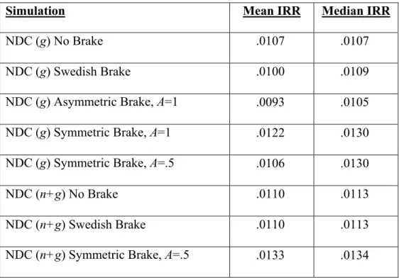
Consider first the performance of the NDC system based on r = g, roughly the Swedish approach without a brake mechanism. As shown in the first row of Table 1, this system provides a mean internal rate of return of 1.07 percent, close to the rate of 1.1 percent for a system in which all variables are constant at their mean values. Note that the IRR is a highly nonlinear function of the variables, so that the mean IRR across stochastic trajectories need not be close to the IRR of the means of the trajectories. The median IRR also equals 1.07 percent for this scheme. However, the need for a brake is quite evident from Figure 2, which shows the distribution of assets-payroll ratios for the system’s first 100 years of operation. The median trajectory has essentially no accumulation of debt or assets. But, with no brake, some trajectories lead to accumulation of debt levels nearly 40 times payroll, clearly an unsustainable level. Indeed, a debt-payroll ratio of nearly 10 is present after 100 years in one-sixth of all trajectories, so this problem is not one limited to extreme draws from the distribution of outcomes. In addition, several trajectories involve substantial accumulation of assets relative to payroll.
6 The Social Security Trustees’ assumption about GDP growth is 1.5 percent (this is from TR04, where it results
from 1.6 percent productivity growth plus 0.2 percent growth in total employment plus the GDP deflator of 2.5 percent minus the CPI deflator of 2.8 percent). But this is not in stochastic equilibrium, the population growth rate is not near 0, and the ratio of covered payroll to GDP is changing over time.
Now consider the NDC system with the Swedish brake in place. As one would expect, imposing such a brake reduces the mean IRR, as shown in the second row of Table 1. The median IRR, though, actually rises slightly.7 As Figure 3 shows, the lower tail of assets-payroll outcomes is raised, as also expected. Indeed, the Swedish balance mechanism is extremely successful in preventing excessive debt accumulation. After 100 years, the 2.5th percentile of the asset-payroll distribution is just -0.26, a debt-payroll ratio of just over ¼. But, even with the periods of acceleration that exist while it is in effect, the balance mechanism does little to restrain the accumulation of assets. Indeed, by cutting off the lower tail of the asset-payroll distribution, the balance mechanism raises both median and mean assets-payroll ratios so that both are substantially positive after 100 years. Indeed, even the 83.3rd percentile is slightly higher, as heading off debt makes the subsequent accumulation of assets levels more likely along a given trajectory.
This upward shift in the distribution of assets over time has an interesting impact on the distribution of internal rates of return by cohort. Figure 4 shows this distribution for the Swedish brake just discussed, for all cohorts with complete lifetimes during the 500-year simulation period. For early cohorts, the lower tail of the distribution of internal rates of return is quite low due to a chance of prolonged downward adjustment of NPW and benefits in the case of low rates of growth. Over time, the likelihood of such an outcome falls; with prior asset accumulation, even a series of bad draws with respect to the growth rate are less likely to drive the balance ratio below 1.0.
7 This result is possible because the brake mechanism has periods during which the growth rates of NPW
accumulation and benefits are accelerated relative to the basic system without a brake. Thus, even though the brake mechanism is designed to reduce benefits overall while in effect, it may have distributional effects across cohorts that reduce the returns of cohorts with IRRs already below the median, while raising the returns of those at the
The Swedish balance mechanism is asymmetric, taking effect only once the balance ratio falls below 1.0. Once in effect, however, the Swedish mechanism does provide for “catch-up” periods of faster growth. A simpler mechanism would eliminate the catch-up phase and apply simply whenever b <1. How different would this even more asymmetric system be from the Swedish system? That is, how significant is the catch-up phase of the Swedish balance
mechanism? Figure 5 shows the asset accumulation pattern under this simple asymmetric brake. As one would expect, the distribution is shifted upward relative to the Swedish system, but only slightly. Consistent with this upward shift, the mean and median internal rates of return are a bit lower for this plan than for the Swedish system (compare the second and third lines of Table 1). Thus, the Swedish system performs very much like a purely asymmetric brake, doing very well at avoiding debt accumulation but actually increasing the possibility of significant asset
accumulation.
To limit asset accumulation in the presence of a brake, a symmetric brake mechanism is needed, to increase accumulations and annuity benefits when the system’s fiscal health is assured, not just to compensate for past periods of cutbacks. A symmetric brake would always be in effect, adjusting benefits and NPW up or down according to expression (4) or (5) regardless of whether b is below or above 1.0. Implementing a symmetric version of the brake leads to more generous benefits for some trajectories, and hence higher mean and median IRRs, as the fourth row of Table 1 shows. (It also eliminates the trend in internal rates of return seen in Figure 4.) The distribution of assets-payroll ratios is similar for the lower tail as under the Swedish and asymmetric brakes, but the upper tail has been pulled down by the brake’s
symmetry, with the 97.5th percentile assets-payroll ratio just below 1.2 after 100 years. Further, both the mean and median assets-payroll ratios stay close to zero. Thus, the NDC system can be
made to be quite stable financially, in both directions, by applying the brake not only when the balance ratio is too low but also when it is too high. This stability holds over the longer term as well, as shown in Figure 6, which exhibits the distribution of assets-payroll ratios over 500 years for the symmetric brake scheme.
Another modification of the brake mechanism is in its strength rather than its symmetry. While rapid adjustment of benefits and NPW growth may provide stability, it may also
concentrate the burdens of fiscal adjustment on relatively few cohorts. We plan to explore the questions of risk-sharing and distribution in subsequent research, but we can consider here the impact of a more gradual adjustment process on the stability of the brake mechanism. Figure 7 shows the distribution of asset-payroll ratios when the brake is symmetric but the adjustment parameter, A, is set equal to 0.5 rather than 1. One can see from a comparison of Figures 6 and 7 that more gradual adjustment does widen the distribution by about a third, but the impact is limited.
Another potential modification of the NDC system involves the computation of the rate of return for NPW accumulations and annuity computations. Even if the average population growth rate is zero, this growth rate can fluctuate, and with this fluctuation the ability of the NDC system to cover benefits. Thus, building population growth into the rate of return should provide greater system stability, ceteris paribus. Figures 8, 9, and 10, and the last three rows of Table 1, present assets-payroll distributions and IRRs for NDC systems based on r = n+g for the no-brake, Swedish-brake and symmetric-brake (A = 0.5) variants.
The impact of this change in the method is most easily seen by comparing Figure 8, the trajectory of debt under the NDC system with no brake and with r = n+g, and Figure 2, the debt trajectory under the system with no brake and r = g. While the assets-payroll distribution still
does not fully stabilize, its range is much smaller, especially in the lower tail. The (2.5, 97.5) range of outcomes is now (-2, +8) instead of (-35, +19). Still, a brake is needed to prevent eventual debt explosion along some paths, and the Swedish brake accomplishes this, as in the previous case of r = g. Again, basing pension calculations on n+g rather than g also
substantially reduces the variation in asset-payroll ratios, as one can see from a comparison of Figures 3 and 9. Even though the upper range of the distribution has been lowered, though, a symmetric brake is still needed to stabilize the up side. Thus, even for the case of r = n+g, a symmetric brake is a sine qua non for system stability in the very long run. Figure 10 shows the trajectory for the symmetric brake with r=n+g and A=0.5. As under the plan with r=g pictured in Figure 7, the distribution of outcomes is quite acceptable over even 500 years. A comparison of the two figures indicates that using n+g in calculating the rate of return is particularly
effective at preventing debt accumulation, a result that was also evident in the earlier comparisons.
Sources of Instability
As we have seen, the basic NDC system, even with Swedish-style net brake, is
financially unstable. Even the NDC system based on setting the rate of return r= n+g requires the application of a symmetric brake to head off substantial asset or debt accumulations on some trajectories. What is causing such instability? One can consider the impact of some sources of uncertainty by eliminating others from the simulations.
In our basic model, uncertainty arises from demographic and economic changes, the latter consisting of fluctuations in the interest rate and the rate of productivity growth.8 These
Figure 2.a and 8.a present 100-year distributions of debt-payroll ratios for both versions of the NDC system (g and n+g) with no brake, corresponding to Figures 2 and 8 and differing from the systems depicted in those figures only in that productivity growth and the interest rate are held constant at their mean values. With only demographic fluctuations present, these new figures show, the distributions of asset-payroll ratios are substantially narrowed. Under the NDC(g) system, the (2.5, 97.5) percentile range at 100 years shrinks from (-35, +19) to (-22, +8); under the NDC(n+g) system, the same range shrinks from (-2, +8) to (-0.5, +2.5). Thus, even with the growth rate g incorporated in the rate of return used in the NDC system’s calculations, this process does not come close to neutralizing fluctuations in that growth rate. Although these comparisons may seem to indicate that demographic fluctuations are an unimportant source of uncertainty relative to productivity growth and interest rates, other comparisons show the dramatic improvement in stability that results from including demographic change, n, in the system rate of return. For example, comparing Figure 8a to Figure 2a indicates that instability as measured by the width of the 95% range is narrowed by a factor of 10 in the n+g system relative to the g system, and comparison of Figure 8 to Figure 2 indicates that this range narrows by a factor of 7 even when the economic variation is included as well. Clearly both the economic and demographic variation are important sources of uncertainty in these NDC systems.
Conclusions
We have considered the financial stability of different variants of a system of Notional Defined Contribution accounts, using demographic and economic characteristics of the United States. In subsequent work, we will consider other aspects of NDC systems, notably their ability
to smooth economic and demographic risks among different generations. Among our findings here are:
1. A system similar to that currently in use in Sweden, which bases rates of return on the growth rate of average wages and utilizes a brake to adjust the rate of return during periods of
financial stress, ensures effectively against excessive debt accumulation but, very much like a simpler asymmetric brake, leads on average to considerable asset accumulation.
2. Only a symmetric brake, which raises rates of return during periods of financial strength, can avoid considerable accumulations of financial assets on some paths. The brake can be more gradual than under the Swedish system and still provide a stable distribution of outcomes. 3. An NDC system in which rates of return are based on total rather than per capita economic
growth is inherently more stable than the basic NDC system, without reference to the brake mechanism in use.
4. A considerable share of the volatility in the financial performance of NDC systems is attributable to economic, rather than demographic, uncertainty.
Evidently stochastic simulation of the system’s finances can reveal aspects of its performance that are not otherwise obvious, and can assist in improving system design. This promises to be a valuable use for stochastic simulation models of pension systems.
References
Alho, J.M., J. Lassila and T. Valkonen. 2005. “Demographic Uncertainty and Evaluation of Sustainability of Pension Systems.” In Non-Financial Defined Contribution (NDC)
Pension Schemes: Concept, Issues, Implementation, Prospects, edited by R. Holtzmann
and E. Palmer, 95-115. Washington D.C.: World Bank.
Booth, Heather. 2006. “Demographic forecasting: 1980 to 2005 in review.” International
Journal of Forecasting 22(3): 547-581.
Holtzmann, R. and E. Palmer, Editors. 2005. Non-Financial Defined Contribution (NDC) Pension Schemes: Concept, Issues, Implementation, Prospects. Washington D.C.: World Bank.
Lee, Ronald. 1993. “Modeling and Forecasting the Time Series of US Fertility: Age Patterns, Range, and Ultimate Level.” International Journal of Forecasting 9: 187-202.
Lee, Ronald and Lawrence Carter. 1992. “Modeling and Forecasting U.S. Mortality.” Journal of
the American Statistical Association 87(419): 659-671, and “Rejoinder,” same issue,
674-675.
Lee, Ronald and Timothy Miller. 2001. “Evaluating the Performance of the Lee-Carter Approach to Modeling and Forecasting Mortality.” Demography 38(4): 537-549.
Lee, Ronald and Shripad Tuljapurkar. 1994. “Stochastic Population Projections for the United States: Beyond High, Medium and Low.” Journal of the American Statistical Association
89(428): 1175-1189.
Lee, Ronald and Shripad Tuljapurkar. 1998a. “Stochastic Forecasts for Social Security,” In
Frontiers in the Economics of Aging, edited by David Wise, 393-420. Chicago:
University of Chicago Press.
Lee, Ronald and Shripad Tuljapurkar. 1998b. “Uncertain Demographic Futures and Social Security Finances.” American Economic Review 88(2): 237-241.
Lee, Ronald D., Michael W. Anderson, and Shripad Tuljapurkar. 2003. “Stochastic Forecasts of the Social Security Trust Fund” Report for the Social Security Administration (January) posted on the web site of the Office of the Actuary.
Legros, Florence. 2003. “Notional Defined Contribution: A Comparison of the French and German Point Systems,” paper presented at the World Bank and RFV Conference on NDC Pension Schemes, Sandhamn, Sweden (Sept. 28-30, 2003).
Palmer, E. 2000. “The Swedish Pension Reform Model – Framework and Issues,” World Bank’s Pension Reform Primer Social Protection Discussion Paper no. 0012.
Settergren, O. 2001a. “The Automatic Balance Mechanism of the Swedish Pension System – A Non-technical Introduction.” Wirtschaftspolitishe Blatter 4/2001: 399-349. Also.: http://www.forsakringskassan.se/sprak/eng/publications/dokument/aut0107.pdf
Settergren, O. 2001b. “Two Thousand Five Hundred Words on the Swedish Pension Reform.” For the Workshop on Pension Reform at the German Embassy, Washington D.C. Swedish Pension System. 2005. Annual Report.
Valdes-Prieto, Salvador. 2000. “The Financial Stability of Notional Account Pensions.” Scandinavian Journal of Economics 102(3), 395-417.
Appendix: Benefits and Taxes under a Simple NDC Plan
This appendix illustrates the relationship between benefits and taxes at a given point in time under a simple version of the Notional Defined Contribution scheme in which the intrinsic rate of return is based on the growth rate of covered wages.
Consider the relationship between taxes and benefits at any given date t under a
simplified version of an NDC system under which the rate of return used to accumulate notional pension wealth and to calculate annuities, rt, is equal to the contemporaneous growth of covered
wages.
Taxes at time t are:
(A1)
(
t L)
t t t t t t W W W T =τ +1+ +2 +...+ + where t j tW + is covered wages in year t for the entire cohort that will retire j years hence and L is
the number of years that individuals work.
For simplicity, assume that each retired cohort receives in benefits the annual real return on its notional pension wealth of rt, so that the cohort’s NPW will stay constant in real terms after
retirement, and its annual payout is constant as well.9 Then aggregate benefits at date t will equal: (A2)
(
1 ...)
1 + + = − − t t t t t t r NPW NPW B9 This assumption implies that a cohort’s benefits per capita grow as the cohort’s population declines and indeed
where t j j t NPW −
− is the notional pension wealth in the year of retirement for cohort retiring in year
t-j. The notional pension wealth at retirement for cohort t-j is:
(A3) + + + + + =
∏
− = − − − − − − − − − − − − − − − 1 1 1 2 1 (1 ) ... (1 ) L l l j t j t L j t j t j t j t j t j t j t j t W W r W r NPW τCombining expressions (A2) and (A3) and comparing the resulting expression with expression (A1), we can see that a sufficient condition for taxes and benefits to be equal is that, for all k
between 1 and L, (A4)
∑
∞∏
= − = − − − − − + = + 0 1 1 ) 1 ( j k l l j t j t k j t t k t t r W r W τ τor, that taxes paid by workers k years away from retirement equal benefits attributable to earnings at the same age for all retirees.
We have assumed that rs equals the growth rate of covered wages between dates s-1 and
s. If we assume in addition that this growth rate is shared by the entire age-wage distribution (i.e., that the relative age-distribution of covered wages remains fixed), then expression (A4) can be rewritten as: (A5) 1 ) 1 ( ) 1 ( ) 1 ( ) 1 ( ) 1 ( ) 1 ( ) 1 ( ) 1 ( 1 1 0 1 1 1 0 1 1 1 1 0 1 1 1 0 1 1 1 0 1 1 = + + + ⇒ + + + = + + =
∏
∑
∏
∏
∏
∑
∏
∏
∏
∑
∏
− = − − ∞ = = − − − = − − − − = − − ∞ = = − − − = − + − + − = − − ∞ = = − − − + k l l j t j j m m t k q q t t k l l j t j j m m t k p p k t k t t t k l l j t j j m m t t k t t k t t r r r r r r r W r r r W r WThe last line of expression (A5) is satisfied if r is constant over time, which reflects the underlying consistency of using the growth of covered wages as a rate of return for the NDC system. If r varies over time, though, expression (A5) will generally not hold. For example, suppose k = 1, corresponding to wages in the year prior to retirement. Then the last line of (A5) reduces to: (A6) (1 )
(
1 (1 ) (1 ) 1 ...)
1 2 1 1 1 1 + + + + + = + − − − − − − t t t t r r r rFrom this, we can see that if the current growth rate used to compute annuities, rt, is greater (less) than the growth rates of covered wages during the accumulation phase, then the expression on the left-side will be greater (less) than 1 and taxes on earnings for those in the year prior to retirement will be inadequate (more than adequate) to cover benefits for retirees based on earnings in the year prior to retirement. Although the results are more complicated for values of k >1, the point is that variations in r over time can cause the NDC system to run deficits or surpluses, the variation being larger the larger is the variation in the growth rate of covered wages. This variation in deficits occurs even under the assumption of a fixed covered earnings age profile; relaxing this assumption adds yet another potential source of variation in the system’s annual deficits.
Table 1. Average Internal Rates of Return
Simulation Mean IRR Median IRR
NDC (g) No Brake .0107 .0107 NDC (g) Swedish Brake .0100 .0109 NDC (g) Asymmetric Brake, A=1 .0093 .0105 NDC (g) Symmetric Brake, A=1 .0122 .0130 NDC (g) Symmetric Brake, A=.5 .0106 .0130 NDC (n+g) No Brake .0110 .0113 NDC (n+g) Swedish Brake .0110 .0113 NDC (n+g) Symmetric Brake, A=.5 .0133 .0134
Figure 1. Ratio of Retirees to Workers, 15 Sample Paths 0 0.2 0.4 0.6 0.8 1 1.2 0 50 100 150 200 250 300 350 400 450 500 Year R ati o of old (>66) to y oun g (2 1-6 6)
Figure 2. Financial Assets/ Payroll (r=g, no brake) -40 -30 -20 -10 0 10 20 0 10 20 30 40 50 60 70 80 90 100 Year Fi na nc ia l A sse ts /Pa yr ol l 0.025 0.167 0.5 0.833 0.975 mean
Figure 3. Financial Assets/Payroll (r=g, Swedish brake) -5 0 5 10 15 20 0 10 20 30 40 50 60 70 80 90 100 Year Fi na ncia l A ss ets/ P ay roll 0.025 0.167 0.5 0.833 0.975 mean
Figure 4. Internal Rates of Return (r=g, Swedish brake) -0.01 -0.005 0 0.005 0.01 0.015 0.02 0.025 0 50 100 150 200 250 300 350 Year Int ernal Ra te o f R eturn 0.025 0.167 0.5 0.833 0.975 mean
Figure 5. Financial Assets/Payroll (r=g, asymmetric brake, A=1) -5 0 5 10 15 20 0 10 20 30 40 50 60 70 80 90 100 Year F ina nc ia l A sse ts /P ay rol l 0.025 0.167 0.5 0.833 0.975 mean
Figure 6. Financial Assets/Payroll (r=g, symmetric brake, A=1) -1 -0.5 0 0.5 1 1.5 2 2.5 0 50 100 150 200 250 300 350 400 450 500 Year Fina ncia l Assets/ P ay roll 0.025 0.167 0.5 0.833 0.975 mean
Figure 7. Financial Assets/Payroll (r=g, symmetric brake, A=.5) -1 -0.5 0 0.5 1 1.5 2 2.5 0 50 100 150 200 250 300 350 400 450 500 Year Fina ncia l Assets/ P ay roll 0.025 0.167 0.5 0.833 0.975 mean
Figure 8. Financial Assets/Payroll (r=n+g, no brake) -2 0 2 4 6 8 10 0 10 20 30 40 50 60 70 80 90 100 Year Fi na ncia l Ass ets/ P ay roll 0.025 0.167 0.5 0.833 0.975 mean
Figure 9. Financial Assets/Payroll (r=n+g, Swedish brake) -2 0 2 4 6 8 10 0 10 20 30 40 50 60 70 80 90 100 Year Fi na nc ia l A sse ts/ P ay ro ll 0.025 0.167 0.5 0.833 0.975 mean
Figure 10. Financial Assets/Payroll (r=n+g, symmetric brake, A=.5) -1 -0.5 0 0.5 1 1.5 2 2.5 0 50 100 150 200 250 300 350 400 450 500 Year Fi na ncia l Ass ets/ P ay roll 0.025 0.167 0.5 0.833 0.975 mean
Figure 2a. Financial Assets/ Payroll (r=g, no brake, constant interest, growth rates)
-40 -30 -20 -10 0 10 20 0 10 20 30 40 50 60 70 80 90 100 Year F ina nc ial Asse ts /P ay roll 0.025 0.167 0.5 0.833 0.975 mean
Figure 8a. Financial Assets/Payroll
(r=n+g, no brake, constant interest, growth rates)
-2 0 2 4 6 8 10 0 10 20 30 40 50 60 70 80 90 100 Year Fi na ncia l Ass ets/ P ay roll 0.025 0.167 0.5 0.833 0.975 mean