Rumor source identification in complex networks

(1)

RUMOR SOURCE IDENTIFICATION IN

COMPLEX NETWORKS

By

Jiaojiao Jiang

Submitted in fulﬁlment of the requirements for the degree of

Doctor of Philosophy

Deakin University

January 2017

(2)

(3)

(4)

DEAKIN UNIVERSITY SCHOOL OF

INFORMATION TECHNOLOGY

The undersigned hereby certify that they have read and

recommend to the Faculty of Science, Engineering and Built

Environment for acceptance a thesis entitled “RUMOR SOURCE

IDENTIFICATION IN COMPLEX NETWORKS” by

Jiaojiao Jiangin partial fulﬁllment of the requirements for the degree of

Doctor of Philosophy. Dated: January 2017 External Examiner: Research Supervisor: Shui Yu Examing Committee:

(5)

(6)

List of Tables

3.1 Summary of Current Source Identiﬁcation Methods. . . 56

4.1 Comparison of Data Collected in the Experiments. . . 71

4.2 Accuracy of Estimating Rumor Spreading Time. . . 85

5.1 Statistics of the Datasets Collected in Experiments. . . 104

5.2 Accuracy of Multi-source Identiﬁcation. . . 107

5.3 Accuracy of Spreading Time Estimation. . . 108

6.1 Statistics of Two Large Networks in Experiments. . . 126

6.2 Statistics of Network Communities and Accuracy of Our Method. . . 132

(11)

List of Figures

1.1 Illustration of time-varying mobile-phone call (MPC) network [44]. Panels (a), and (b) show calls within 3 hours between people in the same town in two diﬀerent time windows. Panel (c) presents the total weighted social network structure, which was recorded by aggregating interactions during 6 months. Node size and colors describe the activity of users, while link width and color represent weight. . . 5 1.2 Illustration of the diﬀusion with two rumor sources. The blue group of nodes

hear the rumor from one source, and the red group hear the rumor from the other source. The yellow nodes are those who receive rumors from both sources. . . 7 1.3 Left: The community construct of a network. Right: The observed network. 9 2.1 Illustration of diﬀerent centrality measures. (A) Degree; (B) Betweenness;

(C) Closeness; (D) Jordan centrality; (E) Eigenvector centrality. . . 13 2.2 The plot of the mean component size excluding the giant component if there

is one (black solid line), and the giant component size (red dashed line), for the ER random network [69]. The mean degreez=p(n−1). . . 15 2.3 The Watts-Strogatz model reproduces the small-world phenomenon by rewiring

edges in a regular network according to the randomness parameter p[108]. 16 2.4 The connectivities of various large real-world networks have scale-free

dis-tributions, (a) actor collaboration graph, (b) the World Wide Web, and (c) the power grid network [9]. . . 17

(12)

2.5 Illustration of three classic epidemic spreading models. (A) SI model; (B)

SIR model; (C) SIS model. . . 20

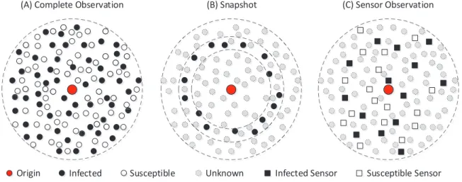
3.1 Illustration of three categories of observation in networks. (A) Complete observation; (B) Snapshot; (C) Sensor observation. . . 24

3.2 Taxonomy of current source identiﬁcation methods. . . 26

3.3 Illustration of wavefronts in the shortest path tree v. Readers can refer to the work “The Hidden Geometry of Complex, Network-driven Contagion Phenomena” [12] for the details of the wavefronts. . . 35

3.4 Sample topologies of two synthetic networks. (A) 3-regular tree; (B) small-world network. . . 43

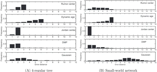
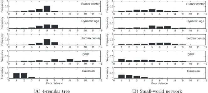
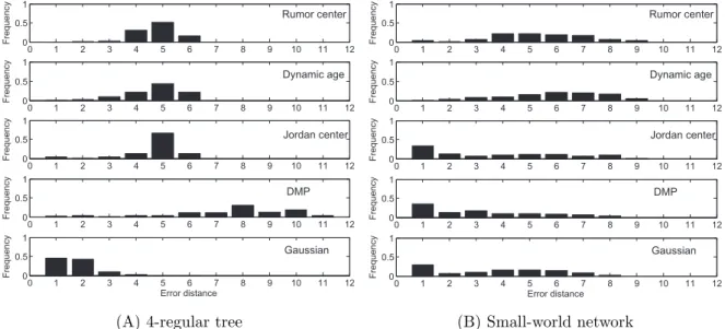
3.5 Crosswise comparison of existing methods on two synthetic networks. 44 3.6 The impact of network topologies. . . 46

3.7 Illustration of diﬀerent propagation schemes. The black node stands for the source. The numbers indicate the hierarchical sequence of nodes getting infected. . . 47

3.8 The impact of propagation schemes: random-walk scheme. . . 48

3.9 The impact of propagation schemes: contact-process scheme. . . 49

3.10 The impact of propagation schemes: snowball scheme. . . 50

3.11 The impact of infection probability. . . 51

3.12 Sample topologies of two real-world networks. . . 52

3.13 Source identiﬁcation methods applied on real networks. . . 53

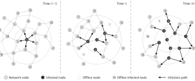
4.1 Example of a rumor spreading in a time-varying network. The random spread is located on the black node, and can travel on the links depicted as line arrows in the time windows. Dashed lines represent links that are present in the system in each time window. . . 61

4.2 State transition of a node in rumor spreading model. . . 62

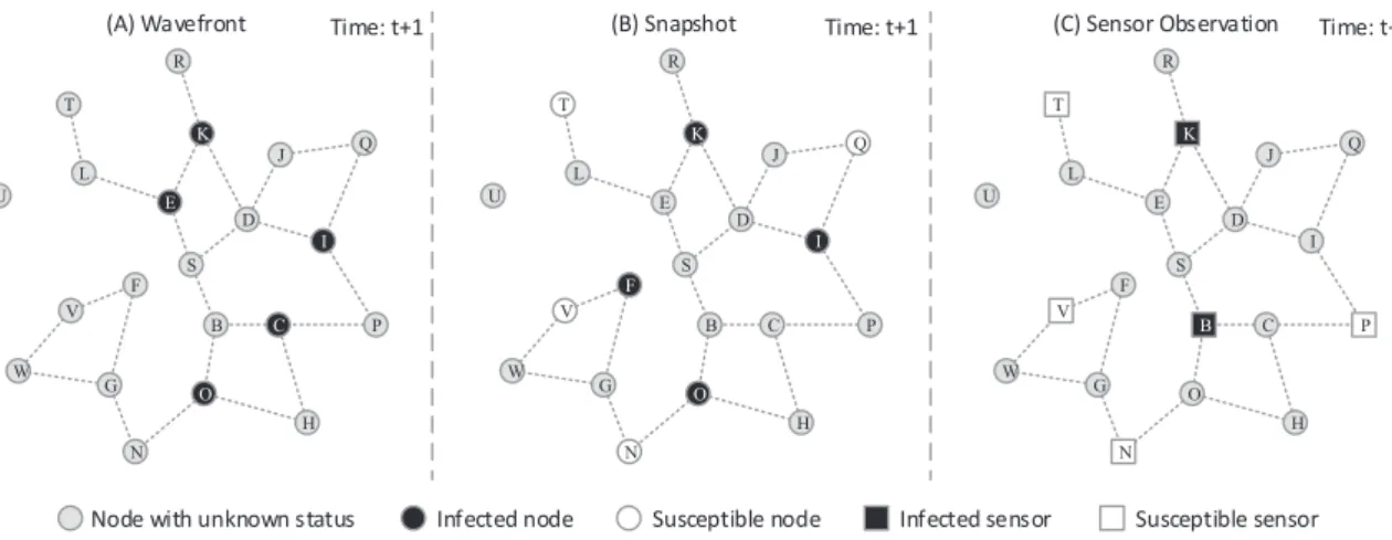
4.3 Three types of observations in regards to the rumor spreading in Fig. 4.1. (A) Wavefront; (B) Snapshot; (C) Sensor. . . 63

(13)

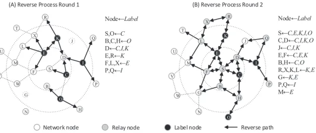
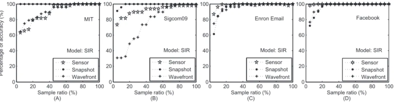
4.4 Illustration of the reverse dissemination process in regards to the wavefront observation in Fig. 4.3 (A). (A) The observed nodes broadcast labeled copies of rumors to their neighbors in time window t; (B) The neighbors who received labeled copies will relay them to their own neighbors in time windowt−1. . . 66 4.5 Accuracy of the reverse dissemination method in networks. (A) MIT; (B)

Sigcom09; (C) Enron Email; (D) Facebook. . . 72 4.6 The distribution of error distance (δ) in the MIT Reality dataset. (A)

Sensor; (B) Snapshot; (C) Wavefront. . . 77 4.7 The distribution of error distance (δ) in the Sigcom09 dataset. (A) Sensor;

(B) Snapshot; (C) Wavefront. . . 78 4.8 The distribution of error distance (δ) in the Enron Email dataset. (A)

Sensor; (B) Snapshot; (C) Wavefront. . . 79 4.9 The distribution of error distance (δ) in the Facebook dataset. (A) Sensor;

(B) Snapshot; (C) Wavefront. . . 80 4.10 The correlation between the maximum likelihood of the real sources and that

of the estimated sources in the MIT reality dataset. (A) Sensor observation; (B) Snapshot observation; (C) Wavefront observation. . . 81 4.11 The correlation between the maximum likelihood of the real sources and that

of the estimated sources in the Sigcom09 dataset. (A) Sensor observation; (B) Snapshot observation; (C) Wavefront observation. . . 82 4.12 The correlation between the maximum likelihood of the real sources and that

of the estimated sources in the Enron Email dataset. (A) Sensor observation; (B) Snapshot observation; (C) Wavefront observation. . . 83 4.13 The correlation between the maximum likelihood of the real sources and that

of the estimated sources in the Facebook dataset. (A) Sensor observation; (B) Snapshot observation; (C) Wavefront observation. . . 84 4.14 The accuracy of estimating infection scale in real networks. (A) MIT; (B)

(14)

5.1 The state transition graph of a node in the SI model. . . 92 5.2 An example of altering an infection graph using eﬀective distance. (A) An

example infection graph with source S. The weight on each edge is the propagation probability. The two dot circles represent the first-order and second-order neighbors of sourceS. The colors indicate the infection order of nodes, e.g., nodes A, C, D and F are infected after the first time tick. Notice that the diffusion process is spatiotemporally complex. (B) The altered infection graph. The weight on each edge is the effective distance between the corresponding end nodes. Notice that the effective distances from source S to the infected nodes can accurately reflect their infection orders. . . 94 5.3 Degree distribution. (A) Power Grid; (B) Yeast; (C) Facebook . . . 104 5.4 The monotonically decreasing of the objective functions. . . 105 5.5 Histogram of the average error distances (∆) in various networks whenS∗

= 2. (A) Power Grid; (B) Yeast; (C) Facebook. . . 106 5.6 Histogram of the average error distances (∆) in various networks whenS∗

= 3. (A) Power Grid; (B) Yeast; (C) Facebook. . . 107 5.7 Estimate of the number of sources. (A) Yeast; (B) Power Grid; (C) Facebook.109 5.8 The correlation between the objective function of the estimated sources and

that of the real sources when S∗ = 2. (A) Power Grid; (B) Yeast; (C) Facebook.. . . 110 5.9 The correlation between the objective function of the estimated sources and

that of the real sources when S∗ = 3. (A) Power Grid; (B) Yeast; (C) Facebook.. . . 111 5.10 The eﬀective distances between the nodes infected at each time tick and

their corresponding sources when S∗ = 2. (A) Power Grid; (B) Yeast; (C) Facebook.. . . 112

(15)

5.11 The eﬀective distances between the nodes infected at each time tick and their corresponding sources when S∗ = 3. (A) Power Grid; (B) Yeast; (C) Facebook.. . . 113 6.1 Illustration of network communities and community bridges. (A) Separated

communities. Community bridges are the nodes associated with between-community edges,e.g., nodes Aand Dconnecting the blue community and the green community. (B) Overlapping communities. Community bridges are not only the nodes associated with between-community edges but also the nodes shared by diﬀerent communities, e.g., nodes H, I and J shared by the green community and the yellow community. . . 119 6.2 Degree distribution of the two large networks. (A) The Mention network;

(B) The Retweet network. . . 127 6.3 The accuracy of the proposed method in identifying diﬀusion sources in two

real large networks. (A) and (C) show the accuracy of our method in the Mention network and the Retweet network having overlapping-community structure with parameterα∈ {0.10,0.15,0.20}. (B) and (D) show the accu-racy of our method in these networks having separated-community structure with parameterβ ∈ {2,3,4}. . . 128 6.4 Community size distribution under diﬀerent parameter setting. (A) and

(B) show the community size distribution in the Mention network and the Retweet network having separated community structure withβ ∈ {2,3,4}; (C) and (D) show the community size distribution in the Mention network and the Retweet network having separated community structure with α ∈

{0.10,0.15,0.20}. . . 131 6.5 The inﬂuence of the ratio of infected sensors in the accuracy of our method

(16)

6.6 Justification of our method on the Mention network. (A) Linear correlation between the relative infection time of sensors and their average effective distance from the diffusion source. Specifically, we let the diffusion start from sources with different degrees: small degree, moderate degree and large degree. (B), (C) and (D) show the correlation coefficient value for each suspect. . . 134 6.7 Justification of our method on the Retweet network. (A) Linear correlation

between the relative infection time of sensors and their average effective distance from the diffusion source. (B), (C) and (D) show the correlation coefficient value for each suspect.. . . 135 6.8 Degree distribution of the four networks. (A) Political Mention; (B) Political

Retweet; (C) Power Grid; (D) Yeast PPI network. . . 138 6.9 Betweenness distribution of the four networks. (A) Political Mention; (B)

Political Retweet; (C) Power Grid; (D) Yeast PPI network. . . 139 6.10 Comparison of the proposed method with other methods in the accuracy

of identifying diﬀusion sources when setting sensors at high-degree nodes in four moderate-scale networks. (A) Political Mention; (B) Political Retweet; (C) Power Grid; (D) Yeast.. . . 140 6.11 Comparison of the proposed method with other methods in the accuracy

of identifying diﬀusion sources when setting sensors at high-betweenness nodes in four moderate-scale networks. (A) Political Mention; (B) Political Retweet; (C) Power Grid; (D) Yeast. . . 141 6.12 The relationship between degree and the average betweenness at each degree

of the four networks. (A) Political Mention; (B) Political Retweet; (C) Power Grid; (D) Yeast PPI network. . . 142 6.13 Linear correlation between relative infection time and average eﬀective

(17)

Acknowledgements

Firstly, I would like to express my deepest gratitude and appreciation to my super-visors Dr. Shui Yu, Prof. Wanlei Zhou, and Dr. Simon James. They have given me so much advise, encouragement, and endless support during the three-year journey of my PhD study at Deakin University. I appreciate all the time they have spent on editing my papers, discussing my research ideas, listening to my problems, and taking away all my doubts and worries. I will always be very grateful for their guidance, support and encouragement.

Secondly, I would like to give my sincere thanks to my research collaborators, Prof. Yang Xiang, and Dr. Sheng Wen. I have acquired a rich set of skills and experiences from their research experiences, knowledge, and meticulous attitude to research during my PhD expedition. Every piece of helpful suggestion makes me better and makes me enjoy research more.

I would also like to thank the academic and general research staﬀ of the School of Information Technology, Deakin University. I would like to give my thanks and appreciation to Ms. Alison Carr and Ms. Lauren Browne for their great secretarial work. Thanks to everyone working in the Research Center for Cyber Security Re-search, I was able to easily access a large collection of Research data to facilitate my research. I also owe a great deal of thanks to my friends who helped me in my study and daily life during my PhD study: Xiao Chen, Dr. Jun Zhang, Prof. Xinyi Huang, and so many others.

I also would like to thank my family for their support and love. Without their everlasting encouragement and understanding, this thesis wouldn’t exist.

Melbourne, Australia Jiaojiao Jiang

(18)

List of Publications

Refereed Journal Articles

1. Jiaojiao Jiang, Sheng Wen, Shui Yu, Yang Xiang, and Wanlei Zhou,

“Iden-tifying Propagation Sources in Networks: State-of-the-Art and Comparative

Studies,” IEEE Communications Surveys and Tutorials, accepted on

Septem-ber 17, 2014.

2. Jiaojiao Jiang, Sheng Wen, Shui Yu, Yang Xiang, and Wanlei Zhou,

“K-center: An Approach on the Multi-source Identiﬁcation of Information

Diﬀu-sion,” IEEE Transactions on Information Forensics and Security, vol. 10, no.

12, 2015, pp. 2616-2626.

3. Jiaojiao Jiang, Sheng Wen, Shui Yu, Yang Xiang, and Wanlei Zhou, “Rumor

Source Identiﬁcation in Social Networks with Time-varying Topology,” IEEE

Transactions on Dependable and Secure Computing, accepted on December 30, 2015.

4. Jiaojiao Jiang, Sheng Wen, Shui Yu, Yang Xiang, and Wanlei Zhou, “The

Structure of Communities in Scale-free Networks,”Concurrency and

Computa-tion: Practice and Experience, accepted on January 1, 2016.

5. Sheng Wen, Jiaojiao Jiang, Yang Xiang, Shui Yu, Wanlei Zhou, and Weijia

Jia, “To Shut Them Up or To Clarify: Restraining the Spread of Rumors in

(19)

vol. 25, issue 12, 2014, pp. 3306-3316.

6. Sheng Wen, Jiaojiao Jiang, Bo Liu, and Wanlei Zhou, “Are the Popular

Users Always Important for the Information Dissemination in Online Social Networks?” IEEE Network, vol. 28, issue 5, 2014, pp. 64-67.

7. Sheng Wen, Jiaojiao Jiang, Yang Xiang, Shui Yu, and Wanlei Zhou, “Using

Epidemic Betweenness to Measure the Inﬂuence of Users in Complex Networks,” Journal of Network and Computer Applications, accepted on November 2, 2016.

8. Haibin Zhang,Jiaojiao Jiang, and Zhi-Quan Luo, “On the Linear Convergence

of a Proximal Gradient Method for a Class of Nonsmooth Convex Minimization

Problems,” Journal of the Operations Research Society of China, vol. 1, issue

2, 2013, pp. 163-186.

Refereed Conference Papers

1. Jiaojiao Jiang, Andi Zhou, Kasra Majbouri Yazdi, Sheng Wen, Shui Yu, and

Yang Xiang, “Identifying Diﬀusion Sources in Large Networks: A Community

Structure Based Approach,” IEEE Trustcom2015, vol. 1, pp. 302-309, 2015.

2. Jiaojiao Jiang, Sheng Wen, Shui Yu, Wanlei Zhou, and Yi Qian, “Analysis

of the Spreading Inﬂuence Variations for Online Social Users under Attacks,”

IEEE GlobeCom2016, Washington, DC USA, December 4-8, 2016.

3. Jiaojiao Jiang, Sheng Wen, Shui Yu, and Wanlei Zhou, “Studying the Global

Spreading Inﬂuence and Local Connections of Users in Online Social Networks,”

IEEE SocialSec2016, Yanuca Island, Fiji, December 7-10, 2016.

4. Sheng Wen, Jiaojiao Jiang, Kasra Majbouri Yazdi, Yang Xiang, and

Wan-lei Zhou, “The Relation between Local and Global Inﬂuence of Individuals in

(20)

5. BoHao Feng, Huachuan Zhou, Hongke Zhang,Jiaojiao Jiang, and Shui Yu, “A Popularity-based Cache Consistency Mechanism for Information-Centric

Net-working,” IEEE GlobeCom2016, Washington, DC USA, December 4-8, 2016.

6. Bo Liu, Wanlei Zhou, Jiaojiao Jiang, and Kun Wang, “K-source: Multiple

Source Selection for Traﬃc Oﬄoading in Mobile Social Networks,” IEEE

(21)

Abstract

In the modern world, the ubiquity of networks has made us vulnerable to various

network risks. For instance, computer viruses propagate throughout the Internet and infect millions of computers. Misinformation spreads incredibly fast in online social networks, such as Facebook and Twitter. Infectious diseases, such as SARS, H1N1 or Ebola, have spread geographically and killed hundreds of thousands people. In

essence, all of these situations can be modeled as a rumor spreading through a

network, where the goal is to find the source of the rumor in order to control and prevent these network risks. So far, extensive work has been done to develop new approaches to effectively identify rumor sources. However, current approaches still suffer from critical weaknesses. The most difficult one is the complex

spatiotempo-ral diﬀusion process of rumors in time-varying networks, which is the bottleneck of

current approaches. The second problem lies in the expensively computational

com-plexity of identifying multiple rumor sources. The third important issue is the huge

scale of the underlying networks, which makes it difficult to develop efficient strategies to quickly and accurately identify rumor sources. These weaknesses prevent rumor source identification from being applied in a broader range of real-world applications. This thesis aims to address these issues to make rumor source identification more effective and applicable.

The ﬁrst issue is overcome by proposing an analytical model for modeling rumor

spreading in dynamic networks. Traditional approaches assume ﬁrm connections

between individuals (i.e., static networks) so that people can trace back along the

(22)

physical mobility and online/offline status of individuals in modeling rumor spreading. Furthermore, we propose a novel reverse dissemination strategy to narrow down the scale of suspicious sources, which dramatically promotes the efficiency of our method. We then develop a Maximum-likelihood estimator, which can pinpoint the true source from the suspects with a high accuracy. Experiment results justify the effectiveness of the proposed method in real-world time-varying networks.

We address the second issue through developing an optimization framework for

multi-source identiﬁcation issue. We adapt K-means from data mining and eﬀective

distance to structure diﬀusion pattern of multi-source rumor spreading. After this,

we formulate an optimization problem for multi-source identification, and develop a fast method to solve the problem. Theoretical analysis proves the efficiency of the proposed method, and the experiment results demonstrate the effectiveness of the proposed method in various real-world networks.

For the scalability issue in rumor source identiﬁcation, we explore sensor

tech-niques and develop a community structure based method. Instead of assigning

sen-sors on high-centrality nodes in traditional methods, we propose placing sensen-sors on community bridges. Thus, we can efficiently record the rumor diffusion between com-munities rather than between individuals. Then, we take the advantage of the linear correlation between rumor spreading time and rumor infection distance to develop a fast method which can locate the rumor source with high accuracy. Theoretical analysis proves the efficiency of the proposed method, and the experiment results verify the significant advantages of the proposed method in large-scale networks.

In summary, this thesis makes three major contributions: 1) propose a novel

ap-proach to identify rumor sources intime-varying networks; 2) develop a fast approach

to identify multiple rumor sources; 3) propose a community-based method to

over-come the scalability issue in this research area. These contributions enable rumor

source identiﬁcation to be applied eﬀectively in real-world networks, and eventually diminish rumor damages.

(23)

Chapter 1

Introduction

1.1

Motivation

With rapid urbanization and advancements in transportation technologies, the world

has become more interconnected. Acontagious disease, like SARS [63], H1N1 [29] and

Ebola [103], can spread quickly through a population and lead to an epidemic [56]. It is crucial to quickly identify the set of epidemic sources, so that potential containment policies can be formulated to prevent further spreading of the disease [92]. In a similar

vein, computer viruses, like Cryptolocker and Alureon [62], on a few servers of a

computer network can quickly spread to other servers or computers in the network and cause a good share of cyber-security incidents [106]. Identifying the servers in the network that are ﬁrst infected allows us to detect the latent points of weaknesses in the computer network, so that preventive measures can be taken to enhance the protection at these points. The source identiﬁcation problem also arises in the study of

misinformation spreading in a social network. A piece of misinformation like Barack Obama was born in Kenya started by a few individuals can spread quickly through the underlying social network [21,78]. In many cases, we are interested to ﬁnd the sources

(24)

of the misinformation. For example, law enforcement agencies may be interested in identifying the perpetrators who fabricate misinformation to manipulate the market prices of certain stocks.

In essence, all of the above examples can be modeled as a rumor spreading in a

network of nodes. In a population network, the rumor is the disease that is transmitted between individuals. In the example of a computer virus spreading in a network, the rumor is the computer virus, while for the case of a misinformation spreading in a social network, the rumor is the misinformation. In this thesis, we focus on the problem of identifying rumor diffusion sources: given a complex network and a partial observation of rumor diffusion, determine the rumor diffusion source(s).

From both practical and technical aspects, it is of great signiﬁcance to identify

rumor sources. Practically, it is important to accurately identify the ‘culprit’ of the rumor propagation for forensic purposes. Moreover, seeking the rumor sources as quickly as possible can find the causation of rumors, and therefore, mitigate the damages. Technically, the work in this field aims at identifying the sources of rumors based on limited knowledge of network structures and the states of a small portion of nodes. In academia, traditional identification techniques, such as IP trace back [91] and stepping-stone detection [93], are not sufficient to seek the sources of rumors,

as they only determine the true source of packets received by a destination. In

the propagation of rumors, the source of packets is almost never the source of the rumor propagation but just one of the many propagation participants [114]. Methods are needed to ﬁnd propagation sources higher up in the application level and logic structures of networks, rather than in the IP level and packets.

(25)

rumor diﬀusion sources. The initial methods were designed to work on particular

networks (e.g., regular tree and regular graphs) and with the diﬀusion following the

traditional susceptible-infected (SI) model [22, 42, 95, 96]. Later, some other works were proposed to deal with particular networks but with different epidemic models, such as the recovered (SIR) model and the susceptible-infected-susceptible (SIS) model [55,59,120,121]. The constraints on particular networks were then relaxed to generic network topologies but still assume that rumors spread along the breadth-first search (BFS) trees of networks [12, 25, 53, 84]. Recently, researchers proposed methods to identify propagation sources by using sensor techniques [1, 82, 94], but they are still restricted in the BFS trees of networks. In the real world, rumor diffusion is a complex process and it does not always follow the ideal BFS-tree spreading scheme. It can be affected by the impacts from the dynamic of individuals, the impacts from the structure of the underlying network, the impacts from other related rumors, etc. Therefore, previous methods of rumor sources identification are far from applying effectively and efficiently in real-world networks.

In many ways, current approaches of rumor source identiﬁcation are facing the following three critical challenges.

• The underlying networks are often of time-varying topology. For example, in

human contact networks, the neighborhood of individuals moving over a geo-graphic space evolves over time, and the interaction between the individuals appears/disappears in online social network websites (such as Facebook and Twitter) [87]. Indeed, the spreading of rumors is aﬀected by duration, sequence, and concurrency of contacts among nodes [13, 104]. Then, can we model the

(26)

way that rumor spreads in time-varying networks? Can we estimate the prob-ability of an arbitrary node being infected by a rumor? How do we detect rumor source in time-varying networks? Can we estimate the infection scale and infection time of the rumor?

• Rumors often emerge frommultiple sources. However, current methods mainly

focus on the identification of a single rumor source in networks. A few approach-es are proposed for identifying multiple rumor sourcapproach-es but they all suffer from extremely high computational complexity, which is not practical to be adopted in real-world networks. In this thesis, we will answer the following question-s correquestion-sponding to multi-question-source identification. How many question-sourcequestion-s are there? Where did the diffusion emerge? When did the diffusion start?

• Another critical challenge in this research area is the scalability issue. Curren-t meCurren-thods generally require scanning Curren-the whole underlying neCurren-twork of rumor spreading to locate rumor sources. However, real-world networks of rumor d-iffusion are often of a huge scale and extremely complex structure. Thus, it is impractical to scan the whole network to locate the rumor sources. We develop efficient approaches to identify rumor sources by taking the structural features of networks and the diffusion patterns of rumors into account, and therefore address the scalability issue.

To address the above challenges, this thesis aims to achieve a breakthrough in rumor source identification to enable its effective applicability in real world applications. The approaches involve the complex network theory, information diffusion theory, probability theory, and applied statistics.

(27)

www.nature.com/

SCIENTIFIC

Figure 1.1: Illustration of time-varying mobile-phone call (MPC) network [44]. Panels

(a), and (b) show calls within 3 hours between people in the same town in two diﬀerent time windows. Panel (c) presents the total weighted social network structure, which was recorded by aggregating interactions during 6 months. Node size and colors describe the activity of users, while link width and color represent weight.

1.2

Research Questions

As presented in the previous section, current studies on rumor source identiﬁcation

encounter three critical challenges: time-varying networks, multiple rumor sources

andscalability issue. In this section, we will introduce the research questions examined in each chapter in detail.

1.2.1

Rumor Diﬀusion in Time-varying Networks

In the real world, it takes diﬀerent periods of time for nodes to transmit information to their neighbors. The temporal dynamic is an important factor, particularly when the propagation concerns human involvements [110]. Let us take the mobile phone call (MPC) network [44] as a example. Fig. 1.1(A) and 1.1(B) show two snapshots of the MPC network at diﬀerent times covering a few hours of calls in a town. The

(28)

two plots capture dynamical interaction patterns not visible from the aggregated net-work representation (Fig. 1.1(C)). Traditional methods of rumor source identiﬁcation

assume the ﬁrm connection between individuals (i.e., the network in Fig. 1.1(C)).

However, this will dramatically overﬁt the actual time-varying network structure. This is also the reason that traditional methods present a low accuracy in identifying rumor sources in real-world networks.

Technically, the temporal dynamic of networks is complex. It involves the impact

of the time zone and the population distribution [18]. Individual habits also strongly affect the temporal dynamic of rumor diffusion. Currently, litter literature considers temporal dynamics of the underlying network where rumors diffuse. We consider these factors in modeling rumor propagation. In other words, we model rumor propagation by considering the realistic temporal dynamics of individuals and their interactions. Based on the innovative model, we can trace back the rumor diffusion source and also predict its future trend. This will make a fundamental contribution to rumor source identification, and open up a new direction of modeling rumor propagation. Therefore, identifying rumor sources in time-varying networks is the first research question to address in this thesis.

1.2.2

Rumor Diﬀusion with Multiple Sources

In the real world, the propagation of rumors often initiates from multiple sources. For example, a contagious disease emerging from a small population can spread geo-graphically and infect hundreds of thousands of people [56]. Culprits employ a botnet to spread computer viruses and ﬁnally infect millions of computers and servers [8,28]. Fig. 1.2 shows an example to illustrate the rumor diﬀusion starting from two sources.

(29)

Figure 1.2: Illustration of the diﬀusion with two rumor sources. The blue group of nodes hear the rumor from one source, and the red group hear the rumor from the other source. The yellow nodes are those who receive rumors from both sources.

One source mainly infects the blue nodes, the other source mainly contaminates the red nodes, the yellow nodes are infected by both sources. Few of current methods are developed for multi-source identification. Some single-source identification methods can be adapted to identify multiple rumor sources. However, they all suffer from the

expensive computational complexity (generallyO(Nk), whereN is number of infected

nodes andk is the number of sources). Therefore, they are not practical to be applied

in real-world networks.

Technically, the methods of single source identiﬁcation cannot be directly used for multiple source cases. This is because the spread initiated from multiple sources can-not be thought of as the superposition of multiple single-source propagation processes. Meanwhile, current multi-source identiﬁcation methods are too computationally

(30)

pattern of multi-source rumor diffusion. This is the crucial factor that we consid-er in developing new methods for multi-source identification. Using the pattconsid-ern of multi-source rumor diffusion, we substantially simplify the multi-source identification problem and develop a fast method to solve this problem. Therefore, the identifi-cation of multiple rumor sources is the second research question to address in this thesis.

1.2.3

Rumor Diﬀusion in Large-scale Networks

In the real world, rumor diffusion often occurs in large-scale networks, such as human contact networks, online social networks, computer networks or the World Wide Web. Let us take a real event on Twitter for an example. On April 15th of 2013, two explosions at the Boston Marathon finish line shocked the entire United States [101]. There were millions of tweets about it, and many of the tweets contained rumors and misinformation. Within a couple of days, multiple pieces of misinformation went viral on various social media. The huge scale of the Twitter network severely challenges traditional rumor source detection methods. Therefore quickly identifying rumor sources in large-scale networks is of great significance in practice.

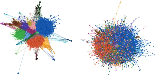
Technically, current methods are too computationally expensive to quickly and accurately detect rumor sources in large-scale networks. This is because most of cur-rent methods require scanning the entire network to locate the rumor sources. More-over, current methods ignore an important fact that rumor diﬀusion often presents a network-driven phenomenon. We show an example in Fig. 1.3 to illustrate one of

the important structures of complex networks − community structure. The left plot

(31)

Figure 1.3: Left: The community construct of a network. Right: The observed network.

in our observation. Appropriately utilizing the structure of networks can facilitate our rumor source detection work in large-scale networks. This is the crucial factor we will consider in developing new methods for identifying rumor sources in large-scale networks. Accordingly, based on the structure of the underlying network, we dramatically decrease the scanning of the entire network to scanning a small commu-nity of the network. Therefore, we propose developing efficient and scalable source identification methods as the final research question in this thesis.

1.3

Thesis Outline

This section aims to establish the structural organization of the thesis. According to

three research issues addressed in this thesis: time-varying networks, multiple rumor

sources and scalability issue, the chapters are organized as follows.

(32)

some basic concepts and network generating models in graph theory, informa-tion propagainforma-tion models and the Maximum-Likelihood Estimainforma-tion method.

• Chapter 3 presents acomprehensive survey on the development of rumor source

identiﬁcation, including relevant concepts, assumptions, and emerging tech-niques in this area. Eﬀorts have been given to identify various research di-rections and emerging research issues.

• Chapter 4 focuses on thetime-varying networks issue in the context of

network-driven rumor propagation. This chapter specifically investigates how to model rumor diffusion in a dynamic network by reducing the network into a series of static network windows. This chapter also proposes an effective two-stage method to detect rumor sources in time-varying networks. The first stage nar-rows down the suspicious rumor sources. The second stage pinpoints the true source from the suspects. The method involves developing a reverse dissemina-tion method to trace back rumor in time-varying networks, and a maximum-likelihood method is explored to compute the probability of the status of arbi-trary individuals.

• Chapter 5 proposes a novel K-center method to address the multiple rumor

sources issue. This chapter focuses on how to efficiently and effectively detec-t muldetec-tiple rumor sources by exploring muldetec-ti-source rumor diffusion padetec-tdetec-terns. Through combining the diffusion patterns and network partition techniques, this chapter formulates the multi-source identification problem as an optimiza-tion problem and proposes a fast method to solve the problem. This chapter

(33)

of rumors sources, (ii)locating the topological places where the rumor emerges,

and (iii) estimating the time when the rumor breaks out.

• Chapter 6 aims at addressing the scalability issue in identifying rumor sources

in large-scale networks. This chapter speciﬁcally explores how to utilize the structural patterns of networks for rumor propagation. With the considera-tion of community structure and sensor techniques in complex networks, this chapter proposed a community-structure based method. Compared with the traditional methods, the proposed community-structure based method dramat-ically decreases the searching scale of rumor sources from the entire network to a small community.

• Chapter 7 summarizes the contributions of this thesis, and presents some

pos-sible suggestions and extensions for further research.

To maintain the readability, each chapter is organized in a self-contained format, and some essential contents, e.g. deﬁnition, are brieﬂy recounted in related chapters.

(34)

Chapter 2

Preliminaries

This chapter provides some preliminary work about rumor source identification. We first introduce some concepts related to complex networks, including node central-ities, network generating models, and community detection methods. Secondly, we introduce three classic information diffusion models adopted in this thesis. Finally, we explain the maximum-likelihood estimation method adopted in this thesis.

2.1

Complex Networks

2.1.1

Node Centralities

Degree Given a node i, the degree of node i is the number of edges connected to

nodei. In general, the larger degree of a node, the more inﬂuential of the node

(see the black nodes in Fig. 2.1(A)).

Betweenness The betweenness of a node stands for the number of shortest paths

from all nodes to all others that pass through the node [31]. Researchers have found some nodes which do not have large degrees also play a vital role in the

(35)

!"##$%&'%% ( ! ) $ * +',-.#/ +',-.#0 )"##)%12%%33%44 ! ) * *"##*5,4%3%44 67&8#9%31':571;#3,<%4 ='<73:';#3,<%4 $"##>,'<:3#*%31':571; ! ) * ?/ ?@ ("##(7&%3A%91,'#*%31':571; @ 0 @ @ / ?0 ?B _? C D E D F @

Figure 2.1: Illustration of diﬀerent centrality measures. (A) Degree; (B) Betweenness; (C) Closeness; (D) Jordan centrality; (E) Eigenvector centrality.

is smaller than nodes A, B, C and D. However, node E is noticeably more

important to information spread as it is the connector of two large groups. To locate this kind of nodes, researchers introduced the measure of betweenness.

Closeness The closeness of a node is deﬁned as the average length of the shortest

path between the node and all other reachable nodes [31, 74]. As shown in

Fig. 2.1(C), this measure discloses the nodes that can rapidly disseminate

information to all the other nodes. This measure concentrates more on the information propagation speed rather than the connectivity of a network [74].

Jordan centrality The Jordan centrality of a node measures the maximum geodesic

distance (shortest-path distance) from the node to a given set of infected nodes

(36)

minimum Jordan centrality. Suppose all the nodes are infected in the graph

in Fig. 2.1(D), then nodes A, B, C are the Jordan centers of the graph with

Jordan centrality 3. Equivalently, Jordan center is equal to the radius of a network [102].

Eigenvector centrality It is deﬁned as the eigenvector of the adjacency matrix

associated to the largest eigenvalue [11, 71]. Equivalently, the eigenvector cen-trality of a node is proportional to the sum of the eigenvector cencen-trality of all its neighboring nodes. In the real world, an important node is characterized by its connectivity to other important nodes. Thus, a node with a high eigen-vector centrality is a well-connected node and has a dominant inﬂuence on the

surrounding network. As shown in Fig. 2.1(E), node V1 and V3 have the

high-est eigenvector centrality in the graph. Readers could refer to [11] for further computation methods.

2.1.2

Network Generating Models

Various models devoted to reproducing the growth and evolution of network topology have been developed to capture diﬀerent characteristics of complex networks. In the following subsections, we will introduce three classic network generating models.

Random Networks

The ﬁrst network generating model proposed in 1959 by Erdos and Renyi [1960]

described the process of growing a random network: n nodes connected by m edges

randomly selected from all n(n−1)/2 possible edges with equal probability p. The

(37)

0 5 Mean degree z 0 2 4 6 8 10

Mean component size

<

S>

0 0.5 1

Giant component size

S

4

1 2 3

Figure 2.2: The plot of the mean component size excluding the giant component if there is one (black solid line), and the giant component size (red dashed line), for the ER random network [69]. The mean degree z=p(n−1).

other key feature is a sudden change of the network connectivity with the increase of

p: when p is small, many clusters are small and isolated, but once p increases to be

larger than a critical value, the network suddenly becomes very dense where almost all the nodes are linked to each other in a giant connected component (see Fig. 2.2).

Small-World Networks

The small-world network originated from the experiment of Milgram [65], in which selected persons were asked to deliver a letter to a target receiver by only passing the letter to their acquaintances. Among all the successful instances, the average length of these communication chains was short, around six steps. The phenomenon is well known as “small-world eﬀect” or “six degrees of separation”. A small-world network has acquaintanceship-based edges and the distance between a random pair of people is smaller than expected. In the real world setting, the small-world eﬀect implies that most of the friends of an individual are people living around, but he may also

(38)

Regular Small-world Random

Increasing randomness Large avg shortest path

High clustering coefficient

Small avg shortest path High clustering coefficient

Small avg shortest path Low clustering coefficient

Figure 2.3: The Watts-Strogatz model reproduces the small-world phenomenon by rewiring

edges in a regular network according to the randomness parameter p[108].

have a few friends far away. People are moving around, but the geographic distance

limits the strength of social relationships. The Watts-Strogatz model was designed

to reproduce the small-world phenomenon by rewiring each link in a regular network

with a probability p [108]. As shown in Fig. 2.3, when p = 0, the network is fully

ordered; when p = 1, every edge is rewired so as to create a random network; when

0 < p < 1, we obtain a small-world network with small average shortest path and high clustering coeﬃcient [108].

Scale-Free Networks

A scale-free network has a power-law degree distribution, commonly seen in many real-world networks, such as the Internet, the ﬁlm actor network, the scientiﬁc col-laboration network, the citation network, and many others (see Fig. 2.4) [4, 9, 69]. Highly unbalanced degree distribution in a social network indicates that, in a large group of people, only a few are extremely popular and most others do not have too

(39)

P(k ) k 100 101 102 103 104 100 10-2 10-4 10-6 10-8 100 101 100 10-1 10-2 10-3 10-4 (a) Actor 100 101 102 103 10-6 10-5 10-4 10-3 10-2 10-1 (b) WWW (c) Powergrid

Figure 2.4: The connectivities of various large real-world networks have scale-free distri-butions, (a) actor collaboration graph, (b) the World Wide Web, and (c) the power grid network [9].

many contacts. It has been suggested to be the most critical feature of social net-works [73].

Among many models that can capture the heterogeneous distribution in connec-tivity [23, 27, 47–49, 73], Barabasi-Albert model was the ﬁrst to generate a scale-free network with two simple mechanisms: continuously adding new nodes into the system (“growth”) and connecting with other nodes with preference to the high-degree ones (“preferential attachment”) [9]. Motivated by the structure of the Web graph, the copying model added a new node into the network and linked it to a random existing node or its neighbors [47, 49]. Another model proposed by Newman et al. [73] aimed to build up a random graph with the arbitrary degree setting. The ranking model grew the network according to a rank of the nodes by any given prestige measure; the probability of linking a target node could be any power law function of its rank, resulting in a power-law degree distribution [27].

(40)

2.1.3

Community Detection

A community is a group of densely connected nodes in a graph. The community structure is claimed to be one key property of various complex networks, suggesting that a network can be partitioned into several (potentially overlapped) clusters so that nodes in one cluster are densely connected internally but not externally; such clustering might derive from common interests of people, geographical divisions of power grids, or functional similarity of proteins [32, 72]. How to detect communities has been widely studied [26], popular methods including modularity optimization [70], Louvain method [10], infomap [89], clique percolation [76], and link clustering [2].

The two methods, Infomap and link clustering, applied in the thesis are introduced

as follows.

Infomap The infomap community detection method is built on the assumption that

a random walker is more likely to be trapped in communities than to trav-el between communities. The path of a random walker can be encoded, and then compressed given a hierarchical network partition so that the encoded description is minimum. The duality between finding community structure in a network and the coding problem is: to find an efficient code, it looks for a

module partitionM ofn nodes intom modules so as to minimize the expected

description length of a random walk. By using the module partition M, the

average description length of a single step is given by

L(M) =q_yH(L) +

m

∑

i=1

piH(Pi), (2.1.1)

(41)

intra-module movements;q_y gives the probability that the random walk

switch-es modulswitch-es on a given step; pi

is the sum of the probability of intra-module

movements inside the module i and the probability of exiting i. The ﬁrst part

of the formula describes the entropy of the movement between communities, and the second part sums up the entropy within each community. Eventually infomap applies computational search algorithm to ﬁnd the best partition as the outcome [89].

Link clustering Diﬀerent from the Infomap method, the link clustering algorithm

aims at discovering overlapped communities in which a node is allowed to be-long to multiple groups. The link clustering algorithm reinvents communities

as groups of links rather than nodes. The set of neighbors of a nodeiis denoted

asNi. Given a pair of links with one shared node,eij andejk, the similarity

be-tween these two links is the Jaccard similarity bebe-tween neighbor sets of distinct nodes:

S(eij, ejk) =

|Ni∩Nk|

|Ni∪Nk|

. (2.1.2)

Then a dendrogram is built up according to these similarities using single-linkage hierarchical clustering and cutting the dendrogram at some level produces the overlapped community structure. Given a partition P = {P1, P2, ..., PC}, a

partition density Dcan be computed by the average partition density weighted

by the fraction of present links in each partition:

D=∑ c mc MDc = 2 M ∑ c mc mc−(nc−1) (nc−2)(nc−1) , (2.1.3)

wheremcandncare the numbers of edges and nodes in the partitionPc,

(42)

S

I

S

I

R

S

I

S

(A)

(B)

(C)

Figure 2.5: Illustration of three classic epidemic spreading models. (A) SI model; (B) SIR model; (C) SIS model.

a maximum partition density.

2.2

Information Diﬀusion Models

Early models concerning communication dynamics were inspired by studies of epi-demic spreading [6, 7, 19, 33, 85]. Similar to how an infectious disease is transmitted among the population, a piece of information can pass from one individual to an-other through social connections and “infected” individuals can, in turn, propagate

the information to others, possibly generating a full-scale contagion. The

susceptible-infected (SI) [45, 46], susceptible-infected-recovered (SIR) [6], and susceptible-infected-susceptible (SIS) [7] models are three classical models in epidemiology, in which the infected population grows exponentially until the rate of infection is balanced by the rate of recovery, or the contagion finally dies off when the recovery rate prevails. As another foundation for this field, different models refer to different scenarios in seek-ing propagation origins. Currently, researchers mainly employ these three epidemic models in rumor source identification:

(43)

2.2.1

Susceptible-Infected model

In this model, nodes are initially susceptible and can be infected along with the propagation of rumor (Fig. 2.5(A)). Once a node is infected, it remains infected

forever. This model focuses on the infection processS →I, regardless of the recovery

process.

2.2.2

Susceptible-Infected-Recovered model

Recovery processes are considered in this model (Fig. 2.5(B)). Similarly, nodes are initially susceptible and can be infected along with the propagation. Infected nodes can then be recovered, and never become susceptible again. This model deals with

the infection and curing process S →I →R.

2.2.3

Susceptible-Infected-Susceptible model

In this model, infected nodes can become susceptible again after they are cured (Fig.

2.5(C)). This model stands for the infection and recovery process S →I →S.

There are also other epidemic models, such as SIRS [99], SEIR [116], MSIR [37], SEIRS [17]. Readers could refer to the work of [113] and [106] for more epidemic models. Future work may consider these models in rumor source identiﬁcation.

2.3

Maximum-Likelihood Estimation

Maximum-likelihood estimation (MLE) [Cowan, 1998] is a method of estimating the

parameters θ of a statistical model M, given the independent observed data X =

(44)

parameters θ is f(xi|θ). Then the likelihood of having parameters θ equals to the

probability of observingX given θ:

L(θ|X) = f(X|θ) =f(x1|θ)f(x2|θ)...f(xn|θ) = Πi= 1nf(xi|θ). (2.3.1) logL(θ|X) = n ∑ i=1 logf(xi|θ). (2.3.2) ˆ

θ= arg max_θ log L(θ|X) = arg max

n

∑

i=1

log f(xi|θ). (2.3.3)

To ﬁnd the optimal parameter ˆθ which best describes the observed data given the

model and thus provides the largest log-likelihood value, we can solve the Eq. (2.3.3) or computationally search for the best solution in the parameter space. This thesis mainly adopts MLE to estimate the probability of a node being a candidate rumor source.

(45)

Chapter 3

Rumor Source Identiﬁcation

This chapter provides an extensive literature review on rumor source identiﬁcation

by tracing research trends and hierarchically reviewing the contributions along each

research line regarding rumor source identiﬁcation.

This chapter consists of four parts. First, we introduce different types of obser-vations on rumor diffusion. Second, for each type of obserobser-vations, we review the existing approaches and analyze their pros and cons. Third, comparative studies are provided according to various experiment settings and diffusion scenarios. Finally, we summarize the analysis and comparative studies, and conclude the perspective research issues in this area.

3.1

Categories of Observations

One of the major premises in rumor source identiﬁcation is the observation of node states during the propagation process. Diverse observations lead to a great variety of methods. According to the literature, there are three main categories of observations:

(46)

!"#$%&'()*+*$,-.*/01+2&3 !4#$531(.6&+ !%#$5*3.&/$,-.*/01+2&3

,/2723 839*:+*; 5<.:*(+2-)* =3>3&?3 839*:+*;$5*3.&/ 5<.:*(+2-)*$5*3.&/

Figure 3.1: Illustration of three categories of observation in networks. (A) Complete

observation; (B) Snapshot; (C) Sensor observation.

sensor observation provide much less information for identifying propagation sources compared with the complete observation.

3.1.1

Complete Observation

Given a timet during the propagation, complete observation presents the exact state

for each node in the network at timet. The state of a node stands for the node having

been infected, recovered, or remaining susceptible. This type of observation provides comprehensive knowledge of a transient status of the network. Through this type of observation, source identiﬁcation techniques are advised with suﬃcient knowledge. An example of the complete observation is shown in Fig. 3.1(A).

3.1.2

Snapshot Observation

A snapshot provides partial knowledge of network status at a given time t. Partial knowledge is presented in four forms: (i) nodes reveal their infection status with

(47)

probability µ; (ii) we recognize all infected nodes, but cannot distinguish susceptible

or recovered nodes; (iii) only a set of nodes were observed at timetwhen the snapshot

was taken; (iv) only the nodes who were infected exactly at timetwere observed. An

example of the 4-th type of snapshots is shown in Fig. 3.1(B).

3.1.3

Sensor Observation

Sensors are firstly injected into networks, and then the propagation dynamics over these sensor nodes are collected, including their states, state transition time and infection directions. In fact, sensors also stand for users or computers in networks. The difference between sensors and other nodes in networks is that they are usually monitored by network administrators in practice. Therefore, the sensors can record all details of the rumor propagation over them, and their life can be theoretically assumed to be everlasting during the propagation dynamics. This is different from the mobile sensor devices which may be out of work when their batteries run out. As an example, we show the sensor observation in Fig. 3.1(C).

In the following three sections, we analyze different techniques for source identifi-cation and discuss their pros and cons. We classify the source identifiidentifi-cation methods into three categories in accordance with the three different types of observations in Section 3.1. The taxonomy of current methods is shown in Fig. 3.2.

(48)

!"#$%&'(%)( *%+,-"(.&"/#0)0-1#0%/ *"/'%,( 23'",41#0%/ 5%678"#"( 23'",41#0%/ */17'$%# 9%,&1/(5"/#", !"''1:"( ;1''0/: 5%/-"/#,0-0#< =+6%,(5"/#", >%-18(,+6%,( -"/#", !+8#078"( ,+6%,(-"/#",' *#1#0'#0-' ?0:"/4"-#%,( 5"/#", @</160-18(A:" !@> B1<"' C1+''01/ !%%/(D18E !"#$%&'()*+#, -$./+)01$#, 2$(/*3#, *0/:8"(,+6%,( -"/#", 9%,&1/(-"/#",( F(*.=(6%&"8 9%,&1/(-"/#",( F(*.(6%&"8 9%,&1/(-"/#",( F(*.*(6%&"8 @</160-( 6"''1:"G71''0/: ?))"-#04"( &0'#1/-" !%/#"(51,8% H%+,G6"#,0-C,""&<(=+8"'

Figure 3.2: Taxonomy of current source identiﬁcation methods.

3.2

Rumor Source Identiﬁcation Based on

Com-plete Observations

In this section, we summarize the methods of source identiﬁcation developed under complete observations. There are two main techniques in this category: rumor center and eigenvector center based methods (see Fig. 3.2).

3.2.1

Single Rumor Center

Shah and Zaman [95], [96] introduced rumor centrality for source identiﬁcation. They assume that information spreads in tree-like networks and the information propaga-tion follows the SI model. They also assume each node receives informapropaga-tion from only one of its neighbors. Since we consider the complete observations of networks, the source node must be one of the infected nodes. This method is proposed for the propagation of rumors originating from a single source.

(49)

as the number of distinct propagation paths originating from the source. The node with the maximum rumor centrality is called the rumor center. For regular trees, the rumor center is considered as the propagation origin. For generic networks, researchers employ BFS trees to represent the original networks. Each BFS tree corresponds to

a probability ρ of a rumor that chooses this tree as the propagation path. In this

case, the source node is revised as the one that holds the maximum product of rumor centrality and ρ.

Analysis In essence, the method is to seek a node from which the propagation matches the complete observation the best. As proven in [95, 96], the rumor center is equivalent to the closeness center for a tree-like network. However, for a generic network, the closeness center may not equal the rumor center. The eﬀectiveness of the method is further examined by the work in [97]. The authors proved that the rumor center method can still provide guaranteed accuracy when relaxing two assumption-s: the exponential spreading time and the regular trees. This method was further explored in the snapshot scenario that nodes reveal whether they have been infected

with probability µ [42]. When µ was large enough, the authors proved the accuracy

of the rumor center method can still be guaranteed. Z. Wang et al. [107] extended the discussion of the single rumor center into a more complex scenario with multiple snapshots. Although snapshot only provided partial knowledge of rumor spreading, the authors proved that multiple independent snapshots could dramatically improve temporally sequential snapshots. The analysis in [107] suggested that the complete observation of rumor propagation could be approximated by multiple independent snapshots.

(50)

considered on a very special class of networks: inﬁnite trees. Generic networks have to be reconstructed into BFS trees before seeking propagation origins. Second, rumors

are implicitly assumed to spread in a unicast way (i.e., an infectious node can only

infect one of its neighbors at one time step). Third, the infection probability between neighboring nodes is equal to 1. In the real world, however, networks are far more

complex than trees, with rumors often spreading inmulticast orbroadcast ways, and

the infection probability between neighboring nodes diﬀering from each other.

3.2.2

Local Rumor Center

Following the assumptions of the single rumor center method, Dong et al. [22]

pro-posed alocal rumor center method to identify rumor sources. This method designates

a set of nodes as suspicious sources. Therefore, it reduces the scale of seeking origins. Method Dong et al. [22] extended the approaches and results in [95] and [96] to identify the source of propagation in networks. Following the deﬁnition of the

rumor center, they deﬁned thelocal rumor center as the node with the highest rumor

centrality compared to other suspicious infected nodes. The local rumor center is considered as the rumor source.

Analysis For regular trees with every node having degreed, the authors analyze the accuracy γ of the local rumor center method. To construct a regular tree, the

degreed of each node should be at least 2. For regular trees, Dong et al. [22] derived

the following conclusions. (i) When d = 2, the accuracy of the local rumor center

method followsO(1/√n), wherenis the number of infected nodes. Therefore, whenn

is suﬃciently large, the accuracy is close to 0. (ii) When the suspicious set degenerates

(51)

to +∞. This means that the minimum accuracyγ is 25% and the maximum accuracy is 30.7%. (iii) When the suspicious nodes form a connected subgraph of the network,

the accuracy γ signiﬁcantly exceeds 1/k when d = 3, where k is the the number of

suspicious nodes. (iv) When there are only two suspect nodes, the accuracy γ is at

least 0.75 if d = 3, and γ increases with the distance between the two suspects. (v)

When multiple suspicious nodes form a connected subgraph, the accuracy γ is lower

than when these nodes form several disconnected subgraphs.

Discussion The local rumor center is actually the node with the highest rumor centrality in the priori set of suspects. The advantage of the local rumor center method is that it dramatically reduces the source-searching scale. However, it has the same drawbacks as the single rumor center method.

3.2.3

Multiple Rumor Centers

Luo et al. [58] extended the single rumor center method to identifymultiple sources.

In addition to the basic assumptions, they further assumed the number of sources was known for the method of identifying multiple rumor centers.

Method Based on the definition of rumor centrality for a single node, Luo et al. [58] extended rumor centrality to a set of nodes, which is defined as the number of distinct propagation paths originating from the set. They proposed a two-source estimator to compute the rumor centrality when there were only two sources. For multiple sources, they proposed a two-step method. In the first step, they assumed a set of infected nodes as sources. All infected nodes were divided into different partitions by using the Voronoi partition algorithm [36] on these sources. The single rumor center method was then employed to identify the source in each partition.

(52)

In the second step, estimated sources were calibrated by the two-source estimator between any two neighboring partitions. These two steps were iterated until the estimated sources become steady.

Analysis Luo et al. [58] are the ﬁrst to employ the rumor center method to identify multiple rumor sources. They further investigate the performance of the two-source estimator on geometric trees [96]. The accuracy approximates to 1 when the infection graph becomes large. This method has also been extended to identify

multiple sources with snapshot observations. Because snapshots only provide partial

knowledge about the spreading dynamics of rumors in networks, W. Zang et al. [118] introduce a score-based method to assess the states of other nodes in networks, which indirectly form a complete observation on networks.

Discussion According to the deﬁnition of rumor centrality of a set of nodes, we need to calculate the number of distinct propagation paths originating from the node set. It is too computationally expensive to obtain the result. Even though Luo et al. have proposed a two-step method to reduce the complexity, the two-step method still

needs O(Nk_{) computations, where} _k _{is the number of rumor sources. This method}

can hardly be used in the real world, especially for large-scale networks.

3.2.4

Minimum Description Length

Prakash et al. [83, 84] proposed a minimum description length (MDL) method for

source identiﬁcation. This method is considered for generic networks. They assumed rumor propagation following the SI model.

(53)

Method Given an arbitrary infected node as the source node, minimum descrip-tion length corresponds to the probability of obtaining the infecdescrip-tion graph. For gener-ic networks, it is too computationally expensive to obtain the probability. Instead,

Prakash et al. [84] introduced an upper bound of the probability and detected the

origin by maximizing the upper bound. They claimed that to maximize the upper

bound is to ﬁnd the smallest eigenvalueλmin and the corresponding eigenvector umin

of the Laplacian matrix of the infection graph. The Laplacian matrix is widely used

in spectral graph theory and has many applications in various ﬁelds. This matrix is

mathematically deﬁned as L=D−A, where Dis the diagonal degree matrix and A

is the adjacency matrix. According to Prakash et al.’s work in [83, 84], the node with

the largest score in the eigenvector umin refers to the propagation source.

Analysis This method can also be used to seek multiple sources. The authors adopted the minimum description length (MDL) cost function [34]. This was used to evaluate the ‘goodness’ of a node being in the source set. To search the next source node, they ﬁrst removed the previous source nodes from the infected set. Then, they replayed the process of searching the single source in the remaining infection graph. These two steps were iterated until the MDL cost function stopped decreasing.

Discussion Due to the high complexity in computing matrix eigenvalues,

gen-erally O(N3_{), the DML method is not suitable for identifying sources}