Crashes and Collateralized Lending

NBER WORKING PAPER SERIES

CRASHES AND COLLATERALIZED LENDING

Jakub W. Jurek

Erik Stafford

Working Paper 17422

http://www.nber.org/papers/w17422

NATIONAL BUREAU OF ECONOMIC RESEARCH

1050 Massachusetts Avenue

Cambridge, MA 02138

September 2011

We thank Joshua Coval, Victoria Ivashina, Martin Oehmke, George Pennacchi, David Sraer, Chris

Rogers, Andrei Shleifer, and seminar participants at EPF Lausanne, MIT Sloan, Northwestern Kellogg,

Princeton University, University of Oregon, University of Pennsylvania, the Spring 2011 NBER Corporate

Finance Meeting, the Summer 2011 SITE Workshop, and the 6th Princeton-Cambridge Exchange

Workshop for helpful comments and discussions. The views expressed herein are those of the authors

and do not necessarily reflect the views of the National Bureau of Economic Research.¸˛¸˛

NBER working papers are circulated for discussion and comment purposes. They have not been

peer-reviewed or been subject to the review by the NBER Board of Directors that accompanies official

NBER publications.

© 2011 by Jakub W. Jurek and Erik Stafford. All rights reserved. Short sections of text, not to exceed

two paragraphs, may be quoted without explicit permission provided that full credit, including © notice,

is given to the source.

Crashes and Collateralized Lending

Jakub W. Jurek and Erik Stafford

NBER Working Paper No. 17422

September 2011

JEL No. G01,G12,G2

ABSTRACT

This paper develops a parsimonious static model for characterizing financing terms in collateralized

lending markets. We characterize the systematic risk exposures for a variety of securities and develop

a simple indifference-pricing framework to value the systematic crash risk exposure of the collateral.

We then apply Modigliani and Miller's (1958) Proposition Two (MM) to split the cost of bearing this

risk between the borrower and lender, resulting in a schedule of haircuts and financing rates. The model

produces comparative statics and time-series dynamics that are consistent with the empirical features

of repo market data, including the dramatic change in financing terms for structured products during

the credit crisis of 2007-2008.

Jakub W. Jurek

Princeton University

Bendheim Center for Finance 211

26 Prospect Avenue

Princeton, NJ 08540

and NBER

[email protected]

Erik Stafford

Graduate School of Business

Harvard University

Baker 371

Boston, MA 02163

[email protected]

An important service provided by financial intermediaries in the support of capital market trans-actions is the financing of security purchases by investors. Investors can buy securities with margin, whereby they contribute a portion of the purchase price and borrow the remainder from the intermedi-ary in the form of a collateralized, non-recourse short-term loan. The risk of the loan depends crucially on three factors: (1) the distribution of economic states; (2) the state-contingent outcomes for the col-lateral value at loan maturity; and (3) the colcol-lateral haircut (or margin) between the market value of collateral and the loan amount. The framework we propose isolates the systematic crash risk exposure of different collateral types (equities, corporate bonds, and CDO tranches), and provides a simple mech-anism for allocating the cost of bearing this risk between a financing intermediary (lender) and investor (borrower), resulting in a schedule of haircuts and financing rates.

A typical loan is collateralized by the underlying security and protected by the borrower’s capital contribution – the collateral haircut, or margin. The haircut protects the lender from changes in the liquidation value of the collateral. Although the liquidation value of an individual security can be affected by myriad market frictions on a day-to-day basis, our focus is on the effect of large market declines (crashes). This approach is motivated by the notion that the intermediaries who provide financing are likely to be well-diversified and have access to relatively efficient hedging strategies enabling them to eliminate the effect of small (diffusive) market moves on collateral values. As such, our framework assumes borrowers post haircuts to immunize lenders against extreme systematic price shocks, or market crashes. This systematic credit risk channel has not been explored in the banking literature, despite the growing role of collateralized lending (e.g. repo market) in the economy, and the widespread interest in ensuring collateral robustness in adverse economic states.

A pervasive feature of capital markets is that extreme price drops – measured relative to recent return volatility – occur with some regularity. Using daily value-weighted US stock market returns from 1926 through 2009, scaled by their lagged standard deviation to construct a time series of Z-scores, we find that observations less than -6 occur every 5 years, on average. These are the economically significant events that collateral haircuts must cover in order for the intermediary to be protected from bearing losses on its loan, and the component of the cost of capital that we investigate.

Unlike most papers in the banking and collateralized lending literature, we specialize to the case where there are no information asymmetries, agency concerns, differences in preferences or beliefs, or other frictions.1 Formally, we assume that the intermediary (lender) is wholly owned by the investor

1_{Some prominent, early papers examining the effect of frictions include: Diamond and Dybvig (1983), Shleifer and Vishny} (1992), Holmstr¨om and Tirole (1997), Bernanke, Gertler, Gilchrist (1996, 1999), Kiyotaki and Moore (1997). Geanakoplos (1997, 2003) emphasizes the endogeneity of haircuts and their sensitivity to perceptions of default. Gennaioli, et al. (2010) present a model of financial innovation based on biased investor beliefs.

(borrower), such that they share the same risk preferences (CRRA utility with a constant relative risk aversion coefficient, γ = 2.5). We then derive a schedule of haircuts and financing rates – measured as spreads above the risk-free rate – which represents the intermediary’s fair charge for providing leverage. Intuitively, the derivation is an application of Modigliani’s and Miller’s (1958) Proposition Two (MM) to an investment fund that owns securities and selects leverage (capital structure). Since the borrower will be indifferent to the choice of capital structure when MM holds, the derived schedule can be thought of as a shadow cost of leverage. We then also examine the borrower’s capital structure choice, if the lender employs an imperfect financing rule (e.g. a credit-rating based spread), such that the cost of leverage is mispriced.

Within our simple framework, spreads/haircuts for economic assets (e.g. equities, corporate bonds, mortgages, etc.) are expected to co-move with one another and proxies for aggregate risk in the time series. A key determinant of the financing terms extended by the lender is the rate at which the value of the collateral declines at the point where the borrower haircut has been wiped out. Securities which have quickly declining recovery values, are expected to: (a) be financed at higher spreads/haircuts; and, (b) respond much more strongly to changes in state variables describing the state of the economy (market volatility). We find that with typical haircuts (e.g. Reg T,H= 0.50) financing spreads on equities are

robustly stable across a range of equity market volatilities. Similarly, our empirical calibration shows that spreads on highly-rated (AA-AAA) corporate bonds remain relatively unchanged, even when haircuts are low (H < 10%). This contrasts meaningfully with the properties of many structured securities. As documented by Coval, Jurek, and Stafford (2009a,b), structured securities can have dramatically different systematic risk profiles (e.g. state-contingent payoffs) than similarly-rated corporate bonds. In particular, the process of tranching can create assets whose values decline rapidly as market conditions deteriorate. As a result, we should expect spreads/haircuts for many types of structured securities to increase much more than for similarly-rated corporate bonds in times of market stress. These predictions broadly parallel the empirical findings of Gorton and Metrick (2009) who examine repo market data from 2007 and 2008. For example, consider the [7,10] tranche referencing the Dow Jones CDX index of investment grade debt (CDX.NA.IG), which was considered by market participants to be a roughly AAA-rated asset. Our model indicates that this securitycannot be used as collateral if we require that the financing spread remain equal to 250 basis points (or less), as market volatilities range between 10-50%. Indeed, Gorton and Metrick (2009) report that during 2008, spreads on this type of collateral averaged 233 basis points with an average haircut of 50%; and – at the peak of the crisis – structured collateral could not be repo-ed at all. Consequently, the extreme change in spreads and haircuts in the

collateralized lending markets is not surprising, when viewed from the perspective of the rapid rise in realized (and implied) equity volatilities.

The framework can also be used to stress test different types of collateral by examining the predicted financing terms as market conditions change. This exercise allows us to isolate two crucial features of the structured finance securities that contributed to their instability, when used as collateral. First, tranche thinness leads to significant volatility in financing terms, even if tranches are backed by high-quality collateral, such as investment grade bonds. Thick tranches (e.g. [7,100]) backed by high-quality collateral inherit much of the stability exhibited by standard corporate bonds. Second, due to the rapid decline in the value of subprime mortgages as economic conditions deteriorate, they represent “poor” collateral. Super senior claims of re-securitizations of sub-prime mortgage RMBS inherit these features, and likewise, will behave poorly when used as repo collateral.

Finally, the framework is helpful for evaluating the notion that many securitizations experienced an increased “information sensitivity” throughout the 2007-2008 credit crisis, leading to concerns over adverse selection and a panicked “run on repo” (Holmstr¨om (2008), Gorton and Metrick (2009), Dang, Holmstr¨om, and Gorton (2010)). This view is largely based on analyses that do not allow for a meaningful systematic risk channel and therefore attribute the entirety of the observed price adjustments to market failure. In contrast, our analysis suggests that the role for state-contingent adverse selection is limited and likely to be diminishing relative to systematic risk exposures as price adjustments become large.

The paper is organized as follows. Section 1 presents a simple framework for valuing the risk of market failure; section 2 empirically characterizes the crash distribution; section 3 describes the cost of capital for specific asset classes; section 4 discusses the implications of the model; and section 5 concludes.

1

Valuing the Risk of Market Failure

In practice many transactions in capital markets bundle the purchase of an asset with the provision of credit. The implicit loan is collateralized by a combination of the (risky) asset being purchased and riskless collateral provided by the purchasing party, known as thehaircut. In this arrangement, the lender effectively provides financing for the difference between the purchase price and the haircut, for which he receives a fee, paid in the form of an interest rate (or spread above the riskless interest rate). The haircut posted by the borrower represents his equity in the transaction. Formally, the parties to the arrangement can bargain over the terms of the loan – duration, haircut and spread – resulting in a schedule of funding

arrangements, which effectively split the risk between the two parties to the transaction.2

To create a meaningful role for risk-sharing, we assume that the security is exposed to jumps in the level of the aggregate equity market index. We interpret these jumps as representing the risk of market failure. From here, to derive the schedule of funding arrangements we need three ingredients: (1) a function describing the consequence of the market failure for the value of the asset, B(·); (2) the frequency,λP_{, and cumulative distribution function,F}P_{(·), of market failures; and (3) a utility function,}

U(·), to analyze the pricing of the underlying risks in the presence of various risk-sharing arrangements. The superscripts,P(Q), denote quantities under the objective (risk-neutral) measure.

1.1 The Model

We introduce the valuation methodology in a simple setting with no financial intermediary. This valuation exercise simply assigns a dollar value to an insurance contract that insures the investor’s wealth from the consequences of an ˜x percent jump in the market index. We denote the pre-jump wealth by

W_t−and the post-jump wealth byW_t(˜x), which will generally depend on the consequence function,B(˜x), describing how the asset is exposed to the crash. To value the jump insurance, suppose there is a claim which pays I(˜x) in the event of a jump with a price of ξ. If the agent buys η units of the claim his terminal expected utility is:

EP t h U ˜ Wt i = (1−πP_)·U(W t−−q·ξ) +πP· Z 1 0 U(Wt(x) +q·I(x)−q·ξ)·fP(x)·dx (1)

whereπP _{is the probability of observing a market failure over some (short) discrete interval of time. At} the optimum the partial derivative of the expected utility with respect toq, evaluated at q = 0, has to equal zero.3 This yields the price of insurance:

ξ = πP_· R1 0 U 0_(W t(x))·I(x)·fP(x)·dx (1−πP_)·U0_(Wt−) +πP·R1 0 U0(Wt(x))·fP(x)·dx (2) 2

Geanakoplos (2003, 2010) examines equilibrium selection along this financing schedule in a setting where agents have heterogeneous beliefs.

3

Bakshi, Madan, Zhang (2006) and Bates (2008) use an indifference pricing methodology to value jump risk in credit default swaps and equity index options, respectively.

The price of jump insurance can also be re-written in terms of the corresponding risk-neutral quantities: πQ _{= π}P_· R1 0 U 0_(W t(x))·fP(x)·dx (1−πP_)·U0_(Wt−) +πP·R1 0 U 0_(W t(x))·fP(x)·dx (3) fQ_{(x) =} U 0_(W t(x))·fP(x) R1 0 U0(Wt(x))·fP(x)·dx (4)

In the case were the loss conditional on a jump is equal to zero, x = 0, the risk-neutral and objective jump probabilities are identical. Using the above expressions, the price of the jump insurance is simply the expected value of its payoff evaluated under the risk-neutral measure:

ξ = πQ_·

Z 1

0

fQ_{(x)·I(x)·dx (5)}

In the presence of an intermediary, who facilitates the provision of leverage – by allowing the investor to borrow funds to finance the purchase of the risky asset – the risk of market failure will be shared between the two parties. The cost of capital to both parties is pinned down from the second proposition of Modigliani and Miller, or equivalently, by valuing the cost of insuring each party against the risk of loss. The consequence of a market failure to the borrower is described by a security-specific function, B(x), which represents a transformation on the loss,x, resulting from the market failure (e.g. the change

in the value of a hedged option portfolio, corporate bond, etc.). If we assume that the risky asset was purchased using financing obtained from a financial intermediary, the borrower’s equity exposure will be limited by the magnitude of the haircut, H. Specifically, the state-contingent loss function for the

borrower is given by:

Ib(x) = min (B(x),H) =    B(x) x <xˆ H x≥xˆ (6)

where ˆx = B−1_{(H). In other words, ˆx is the minimal equity index jump necessary to wipe out the}

borrower’s equity capital, H, in the trade, and expose the lender to a loss. We will generally normalize the consequence function and haircuts, such that they correspond to a $1 position in the risky security. Consequently, the borrower’s leverage – or ratio of assets to equity – is given by H−1_{. To derive the}

cost of capital for the borrower and the lender, we value the cost of insuring each party against the losses stemming from a market failure. By MM, the sum of these dollar costs equals the cost of insuring the unlevered strategy, (5). Therefore, the lender’s charge can be simply obtained by differencing the

borrower’s cost of capital from (5): ξb = πQ· Z 1 0 fQ_(x)·I b(x)·dx = πQ_{·H ·1−F}Q_(ˆx)+EQ_{[B(x)|x <xˆ]·F}Q_{(ˆx) (7)} ξl = ξ−ξb =πQ· EQ_{[B(x)|x >xˆ]− H·1−F}Q_{(ˆx) (8)}

The dollar lender fee is given by the product of three terms: the probability of observing a market failure (πQ_{), the likelihood that the haircut will be exhausted in the event of the market failure, 1−F}Q_(ˆx)

, and the expected loss to the lender as a result of the haircut being exhausted,EQ_{[B(x)|x >xˆ]− H. The} final term is bounded between zero (no credit risk) and 1− H, where the asset loses all value conditional

on the jump, x, exceeding the threshold ˆx. The latter situation describes a levered position in a binary option (or digital tranche), where – if the index jumpxcauses the option to fall out-of-the-money at the expiration date – the borrower’s capitalH is wiped out, and the lender bears the remainder of the loss, 1− H.

It will also be convenient to express the lender’s fee as a percentage of the loan amount:

ξl 1− H = π Q_·1−FQ_(ˆx)· EQ_{[B(x)|x >xˆ]− H} 1− H (9)

Holding risk preferences and crash distributions constant, the largest interest rate is obtained when the third term is equal to unity. In this scenario, the lender’s charge – expressed as a continuous-time flow rate – is given by λQ _{· 1−F}Q_{(ˆx)·dt, where λ}Q _{is the annualized risk-neutral market failure arrival} intensity. This case corresponds to financing a security that becomes worthless following a market crash

x >xˆ.

To gain further intuition regarding the lender’s fee – or, equivalently, the financing rate – we can approximate the consequence function,B(x), around the critical value, ˆx, at which the borrower’s haircut is wiped out. Assuming the consequence function is differentiable we have:

ξl ≈ πQ· 1−FQ_(ˆx)· ∂B ∂x x=ˆx ·EQ_{[(x−xˆ)|x >xˆ] (10)}

where we have made use of the fact that ˆx=B−1_{(H). The above approximation can also be rewritten}

as: ξl ≈ πQ· ∂B ∂x x=ˆx ·EQ (x−xˆ)+ (11)

This formula conveys the intuition that the lender’s exposure is captured by the likelihood of a systematic crash, πQ_{, and his exposure to this crash. The exposure can be further represented as a portfolio of} call options onlosses on the aggregate equity index, struck at the critical value, ˆx, at which the haircut is wiped out (third term). The “quantity” of these options is measured by the slope of the crash consequence function,B(x), around the critical index return (second term). If the consequence function is steep around the critical point, the lender anticipates market failures to precipitate larger losses, resulting in commensurately higher financing rates for any given haircut level, H. As we show later, securities such as traditional corporate bonds and structured finance securities can have significantly different consequence function slopes around the critical point,B0(ˆx), even though they share identical credit ratings. This difference turns out to be a key ingredient in explaining the differences in the dynamics of financing rates (and haircuts) observed for various collateral types during the credit crisis of 2007-2008.

1.2 A convenient parametrization

In order to gain greater transparency and facilitate empirical implementation, it will be convenient to specialize the formulas derived in the previous section to a particular case of the utility function,

U(·), and crash distribution, FP_{(·). Specifically, we will assume that the agent has CRRA utility with}

relative risk aversion, γ, and the distribution of crashes on the market index sustained as a result of market failure has a beta distribution with parameters (a, b). Moreover, since we have assumed that the investor (borrower) owns the intermediary (lender) and there are no market frictions, we can carry out valuation as if in a representative agent setting, with the agent’s wealth being wholly invested in the aggregate wealth portfolio. With this setup, the representative agent’s wealth following a market failure (jump),Wt(x), is given byWt−·(1−x). The resulting risk-neutral jump probability,πQ, can be derived by taking the expression from the previous section and dividing the numerator and denominator byW_t−−γ to obtain: πQ _{= π}P_· R1 0(1−x) −γ_·fP_{(x;a, b)·dx} (1−πP_{) +π}P_·R1 0(1−x)−γ·fP(x;a, b)·dx =πP_· Γ(a+b)·Γ(b−γ) Γ(b)·Γ(a+b−γ) (1−πP_{) +π}P_·Γ(a+b)·Γ(b−γ) Γ(b)·Γ(a+b−γ) (12)

Conveniently, we can also show that the risk-neutral distribution of market failures is likewise a beta distribution but with shifted parameters, (a, b−γ):

fQ_{(x) =} (1−x) −γ_·fP_{(x;a, b)·dx} R1 0(1−x)−γ·fP(x;a, b)·dx = Γ(a+b−γ) Γ(a)·Γ(b−γ) ·x a−1_·(1−x)b−γ−1_{·dx (13)}

As a result, the mean loss in aggregate wealth resulting from the market failure can be evaluated in closed-form under both measures from:

µP ₌ a

a+b and µ

Q₌ a

a+b−γ (14)

The price of an insurance claim that completely hedges the jump risk,I(x) =x – expressed per unit of wealth,W_t−, exposed to the jump – is given by:

ξ = πQ_·

Z 1

0

fQ_{(x)·x·dx=π}Q_· a

a+b−γ (15)

A risk-averse representative agent would therefore be willing to give up a fraction,πQ_·µQ_{, of his wealth}

to hedge the exposure to market failure risk. On the other hand, if the agent were risk-neutral the price of jump insurance would be equal to a fraction πP_·µP _{of total wealth, i.e. equal to the unconditional}

expected loss due to market failures. The approximation of the lender’s fee, (11), can also be further elaborated to yield: ξl ≈ πQ· ∂B ∂x x=ˆx · a a+b · 1−FQ_{(ˆx;a+ 1, b)−xˆ·1−F}Q_{(ˆx;a, b)} (16)

2

Characterizing the Crash Distribution

The framework is based on a frictionless capital market with the exception of the crashes. In these episodes, the market is not functioning as it normally does. The primitive feature of such an event is that it meaningfully interferes with the market participants’ ability to dynamically eliminate their net systematic exposure. We empirically investigate these situations from two basic perspectives. First, we suppose that the market structure is highly robust, but information can be released overnight. While the market is closed overnight, prices are unable to smoothly incorporate information, which creates the possibility of a discrete move in each overnight period. This creates a type of discretization studied by Bertsimas, Kogan, and Lo (2000, 2001) that manifests itself in hedging errors. The borrower is required to post collateral against these hedging errors.

Second, we suppose that the market is typically robust, but that it can occasionally fail. In this view, market failures are rare, but can be associated with large market declines.4. These are significant

4

This is distinct from the “rare economic disasters” perspective of (Rietz (1988), Barro (2006, 2009)). These occur on a considerably longer time scale than the 1-day or overnight crashes considered above, but are important in that they significantly reduce aggregate wealth and therefore risk bearing capacity for outstanding securities. In some sense, this is what the financial system has to survive even if the individual agents do not view this to be their own problem. Barro (2006) estimates that the probability of these rare economic disasters is around 2% per year with a GDP contraction of

events because dynamic hedging strategies can be highly compromised in these situations, leading to ruinous losses. For example, on October 19, 1987, the US value-weighted stock market index declined 17%, following a 10% decline the previous week. Many have argued that liquidity disappeared over this period (for example, Amihud, Mendelson, and Wood (1990)), suggesting that intraday hedging was severely impaired during this event.

To empirically identify crashes from the daily data we employ a simple threshold rule based on Z-scores. In particular, we calculate Z-scores by scaling each return by the standard deviation of lagged returns, in order to eliminate the effects of stochastic volatility. We then use a threshold of -6 to classify daily returns associated with a Z-score below this threshold as crashes (A¨ıt-Sahalia (2004) motivates this cutoff rule). The idea behind using Z-scores to identify extreme events is twofold. First, this measure captures the idea of the crash being highly unusual relative to what was expected going into the situation. In other words, a 5% daily return is highly surprising following 3 months of 0.5% daily volatility, but not if recent daily volatility has been 3%. Second, to the extent that this measure is stable through time, it represents a practical method for producing a conditional forecast of the crash distribution, since the only input is current volatility,σt.

As noted in the previous section, we rely on the beta distribution for analytical convenience.5 The following procedure is used to estimate a conditional crash return distribution. First, we assume that the empirical Z-score distribution, g(Z), is stable across time. Second, we convert the empirical Z-score distribution to a conditional crash return distribution by computing the corresponding losses as,

x= 1−exp (σt·Z). Finally, we fit a beta distribution to the conditional crash return distribution, placing

particular emphasis on matching the tails. Specifically, we assume that the largest observed Z-score cor-responds to thep-th percentile of the population crash distribution and then select the beta distribution parameters that minimize the squared deviations between the empirical and analytical distributions at the median and thep-th percentile. This fitting procedure mitigates the potential of standard moment-matching methods to underestimate the true risk of severe events, due to the historically favorable in-sample experience of U.S. equities (“peso problem”).

In order to assign a population percentile, p, to the largest observed Z-score, we draw on extreme value theory. According to this theory, conditional on being in the tail of a distribution, returns obey a generalized Pareto law – a prediction which has considerable empirical support in U.S. equity return data

15% to 60%

5_{Our results are robust to an alternative approach in which we fit agammadistribution to the Z-scores, and subsequently} scale it by the prevailing volatility,σt, to obtain the relevant log return distribution. In fact, it is possible to show that if

crash returns are beta distributed, the corresponding Z-scores will approximately follow a gamma distribution for modest return realizations.

(Gabaix (2009)). Using maximum likelihood we fit the parameters of the generalized Pareto distribution to the extreme Z-scores and then invert a likelihood ratio test to obtain the joint confidence interval for the parameter estimates. This also yields the corresponding confidence interval for the population percentile,p, of the largest Z-score observed in our sample. For example, in daily data the most severe event corresponds to a Z-score of -15.5, and the estimated 95% confidence interval for p ranges from 79% to 100%. Since lower percentile values imply the population distribution assigns significantly more weight to events evenmore extreme than the worse event observed the dataset, we conservatively assign the largest Z-score observed in-sample to the 95th percentile of the fitted distribution.

2.1 Overnight Returns for the S&P 500 Index

The return data are based on high frequency (5-minute intervals) price observations on the S&P 500 Index from 1983 through 2009 (5,300 overnight observations) obtained from TickData. We define the overnight return for day t as the difference between the log opening price on dayt and the log closing price on dayt−1. Weekend returns are identified as those having more than one calendar day between the opening price and the previous closing price. Prior to 2008, the minimum overnight return is -2.4% and since then it is -5.9%. This already suggests that the contribution of this phenomenon to observed lender financing rates is likely to be small since the lender is unlikely to sustain a loss from crashes of these magnitudes.

The overnight Z-scores are calculated by scaling the overnight return by volatility. Volatility is calculated from the previous 390 intraday returns (5 trading days) and scaled in two ways to account for the time elapsed overnight. The first scaling is by the square root of the elapsed calendar time in the overnight period. The second scaling accounts for the elapsed effective time in the overnight period. Consistent with previous research, we find that the elapsed effective time overnight is considerably less than the elapsed calendar time (see French and Roll (1986), Amihud and Mendelson (1987), and Lockwood and Linn (1990)). We find that, on average, roughly 30% of a trading day’s return volatility is realized in the overnight return, while accounting for 73% of the elapsed calendar time. Despite the additional calendar time inherent in weekends, we find that these periods contribute no more than ordinary overnight periods to realized return volatility, on average. In our analysis we assume that the effective time in overnight and weekend period is equal to 150 minutes, such that the equivalent of 540 minutes of trading time elapses in a trading day (time between consecutive market closings). There are no overnight returns associated with a Z-score below -6 using either scaling rule, indicating that no overnight crashes have been realized in the S&P 500 Index since 1983.

2.2 Daily Returns on the Value-Weighted Market Index

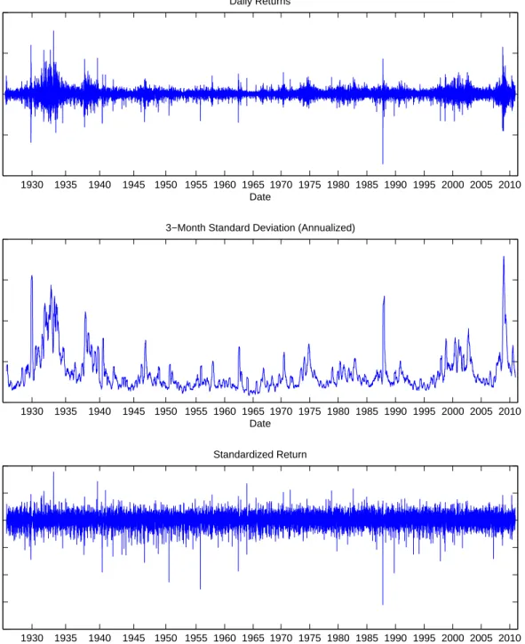
The daily return data come from CRSP and are based on the value-weighted index of US stocks from 1926 through 2010 (22,527 observations). We scale each daily return by the standard deviation of the past 63 returns (3 months) to calculate a Z-score. Again, we then use a threshold of six to classify daily returns associated with a Z-score below this threshold as crashes.

Figure 1 displays the time series of daily returns, volatility, and Z-scores. October 19, 1987, was only 1 of 19 days where the realized daily loss on the stock market was associated with a Z-score below -6. Six of these events have occurred in the last third of the sample period, including the most severe, consistent with the notion that the empirical “crash” distribution is reasonably stable and not much altered in the modern era. This empirical crash distribution implies an annual crash probability of nearly 20% (1−(1−p)252 = 19.15%; wherep= 0.0009 = ₂₂₅₂₇19 ); the corresponding annualized crash intensity equals

λP _{= 0.2126.}

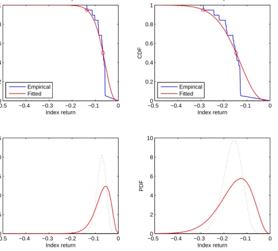
The calibration, where matching the tails is given high priority, takes as inputs the empirical Z-score distribution and the prevailing volatility. Table 1 reports the calibrated beta distribution parameters for a range of index volatilities, set on the basis of the percentiles of the CBOX VIX index time series. By construction, log crash returns scale linearly with the prevailing volatility in our framework. This feature is typical of many jump-diffusion option pricing models used in the equity option literature (e.g. Bates (2000), Pan (2002)). As a result, the standard deviation of crash losses, x, grows roughly linearly with volatility, such that the jump share of variance is essentially constant. For moderate levels of volatility, the 95th percentile crash size – conditional on volatility – is approximately equal to the current level of annualized volatility. Figure 2 displays the calibrated daily crash return distribution at an annualized volatility of 15%, which we will take as our baseline in many of the analyses that follow, as well as at 35%. For comparison, the bottom panel also displays the crash distributions obtained by applying a standard maximum likelihood fitting procedure.

2.3 Implications for aggregate quantities

The presence of a jump component in the return dynamics in the aggregate equity index, influences the total equity volatility and risk premium. The contribution of the shock to the instantaneous index return variance – which is comprised of the diffusive return variance (σ2_t) and jump return variance – is

given by: VarPh_x·dJ(λP₎i _{= π}P_· a·(a+ 1) (a+b+ 1)·(a+b) −πP2_· a a+b 2 ≈ a·(a+ 1) (a+b+ 1)·(a+b) ·λ P_{·dt (17)}

As argued in the previous section, the parameters of the beta distribution, (a, b), will generally themselves be time-varying and depend on the level of the diffusive volatility,σt. A noted earlier, the contribution of

discontinuous moves to total (instantaneous) quadratic variation – measured as a ratio of jump variance to total quadratic variation – is roughly constant in our model (Table 1). With a diffusive volatility of 15% (35%) the total index volatility is roughly equal to 15.44% (35.89%).

In a jump-diffusion setting the total equity risk premium will be comprised of compensation for diffusive risk, and a premium for jump risk. In a standard CAPM setting the compensation for diffusive risk is equal toγ·σ2_t. However, since our setting focuses explicitly on jump risk, this component of the risk premium plays no role in the paper’s results. The contribution of jumps to the equity risk premium is measured by the difference in the expected excess return to bearing jump risk, and is given by:

φrp = πQ· a a+b−γ −π P_· a a+b ≈ Γ(a+b)·Γ(b−γ) Γ(b)·Γ(a+b−γ) · a a+b−γ − a a+b ·λP_{·dt (18)}

For example, with a risk aversion,γ, of 2.5, and a baseline volatility of 15%, the diffusive risk premium would be equal to 5.62% per year, with jump risk contributing an additional 41 basis points. Unlike the share of jumps in total variance, the contribution of the jump risk premium in the total equity risk premium is increasing in the level of diffusive volatility (unreported results).

3

The Crash Risk Cost of Capital for Various Securities

This section uses the model derived in Section 1 to investigate financing arrangements – haircut and spread pairs – for equities and fixed income securities (corporate bonds and structured finance assets). A key ingredient in this analysis are the crash consequence functions,B(x), of these assets. These functions describe the change in the value of the asset in response to a market decline of magnitude,x. In general, the change in the value of the asset depends on the crash magnitude through two channels: (a) its effects on the state-contingent payoff function; and, (2) its effect on state variables that affect state prices. In our case, the the state variables are the equity market volatility,σm(x), the the aggregate risk aversion

form:

B(x) = V (t, x, σm(x), γ)−V t−, x= 0, σm(x= 0), γ

(19)

In the case of equities, which we use to introduce the framework, we will specify the crash consequence function directly using a market model. In the case of fixed income securities, which constitute the bulk of the assets used in repo markets, we construct the crash consequence functions by separately describing the asset-specific payoff functions and state prices. This allows us to investigate in greater detail, which state-contingent payoff profiles are likely to enhance collateral stability, which we define as low volatility in spread-haircut pairs over the range of state variables. Finally, we illustrate how the use of simple rules of thumb – e.g. based on credit ratings – can lead to situations where securities are financed at incorrect spreads/haircuts, creating a motive for borrowers to hold mispriced assets.

Our focus is exclusively on the robustness of the asset value to rare, but generally large, market crashes, which we identify using the procedure in Section 2. In this setting, collateral haircuts are applied by lenders in order to mitigate their exposure to aggregate crash risk. This contrasts with approaches that examine collateral in the context of daily mark-to-market volatility, or liquidity risk. Given the central role of collateralized lending in capital markets, ensuring their robustness in time of severe market stress is likely to be of interest to regulatory agencies.

3.1 Equity

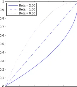
Investing in individual equities on margin represents a prototypical strategy involving lender financing and exposure to aggregate equity risk. We describe each stock using its beta to the aggregate index,β, which is assumed to apply identically to diffusive and jump shocks. The consequence function for a $1 investment in the equity, B(x), is given by:

B(x) = exp{β·ln(1−x)} −1 = (1−x)β−1 (20)

This specification preserves the limited liability of the investment in the individual security, and ensures that a zero percent index return is equal to a zero percent return on the individual security. Moreover, when β = 1 the equity consequence function is equal to −x, i.e. the index loss. The cost of insuring

losses on this strategy,I(x) =−B(x), is given by:

ξ = πQ_· 1−Γ(a+b−γ)·Γ(b+β−γ) Γ(b−γ)·Γ(a+b+β−γ) (21)

Now suppose the investor establishes a levered position in the equity by posting collateral, H, and borrowing the balance of the $1 purchase price from an intermediary. Given the collateral choice, H,

the critical index return at which losses on the levered equity position exceed the collateral is:

ˆ

x = 1−(1− H)β1 ₍₂₂₎

The comparative statics for ˆx are illustrated in Figure 3. Panel A shows the critical crash size that exhausts the borrower’s capital as a function of the underlying equity beta for three different margin rules. Reg T margin requires a collateral haircut of 50% to initiate an equity position. Portfolio margin requires a collateral haircut of 25% for individual equities and 10% for a broad highly capitalized equity index. For an individual equity with a market beta of 1, a lender extending leverage under portfolio margin is completely protected against crashes until the crash size exceeds 25%. Empirically, market betas for individual equities are rarely reliably larger than 2. For a stock with a market beta of 2, the lender is crash protected until the crash size exceeds 13.4%. Panel B shows how ˆx varies as a function of the collateral haircut for three equities with different market betas. When market beta is 1, there is a one-for-one tradeoff between collateral and crash protection for the lender. The lender is protected against larger (smaller) crashes when the stock’s market beta is less (larger) than 1.

The cost of insuring the levered investment can be obtained by applying (7):

ξb = πQ· FQ_{(ˆx;a, b−γ)−}Γ(a+b−γ)·Γ(b+β−γ) Γ(b−γ)·Γ(a+b+β−γ) ·F Q_{(ˆx;a, b+β−γ) +} +H ·1−FQ_{(ˆx;a, b−γ) (23)}

The (up-front) fee paid by the borrower to the lender for providing financing can then be obtained as the difference between the cost of insuring the unlevered strategy and the cost of insuring the losses on the levered investment, ξl = ξ−ξb. This quantity is typically quoted in term of an interest rate (or

spread), which can be obtained by expressing ξl as a fraction of the loan amount, 1− H.

In order to derive the cost of capital for the borrower and lender, we first need to compute the dollar loss each party expects to sustain as a result of market failure. These quantities can be obtained by using the formulas above, but settingγ = 0, since a risk-neutral agent would simply charge the expected

loss: ξ∗ = πP_· 1−Γ(a+b)·Γ(b+β) Γ(b)·Γ(a+b+β) (24) ξ∗_b = πP_·FP_{(ˆx;a, b)−} Γ(a+b)·Γ(b+β) Γ(b)·Γ(a+b+β) ·F P_{(ˆx;a, b+β) +H ·1−F}P_{(ˆx;a, b) (25)}

The cost of capital to each party is then given by:

φb=

ξb−ξ_b∗

H and φl =

ξl−ξ∗_l

1− H (26)

Note that – unlike the interest rate (or spread) on the margin loan – the lender’s cost of capital is adjusted for losses sustained due to insufficient collateral coverage. In other words, the lender must charge a spread that grosses up the cost of capital to cover expected losses.

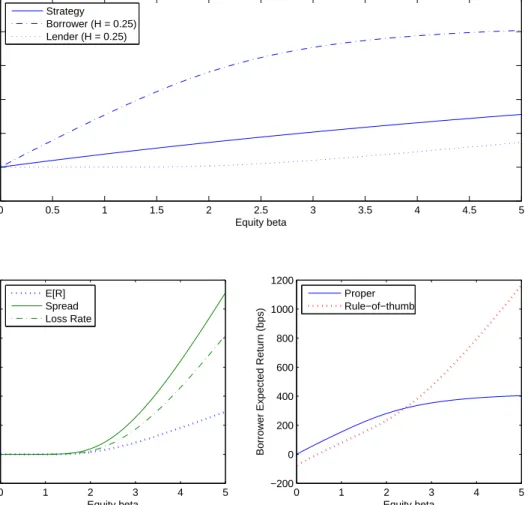
We now use this framework to investigate the properties of the crash component of the cost of capital for equities. Figure 4 shows the crash component of the cost of capital for equities with various market betas and demonstrates how the portfolio margin rule (H = 25%) adjusts the cost of capital for the lender and the borrower. For a stock with a market beta of 1, the security-level (unlevered) cost of capital is 39 bps and increases nearly linearly with market beta, reaching 73 bps for a stock with market beta of 2. With this relatively high collateral haircut, the borrower bears the majority of the crash exposure until market beta gets very high, and consequently has a relatively high cost of capital. The borrower’s cost of capital is 154 bps for a stock with a market beta of 1 and 281 bps for a stock with a market beta of 2. The lender’s margin loan is nearly riskfree over the empirical range of stock betas (0-2), producing lender costs of capital of less than 1 bp for stocks with a market beta of 1 and of only 4 bps for stocks with a market beta of 2. As the market beta increases above 3, the lender bears more of the crash risk so the borrower’s cost of capital increases slowly with beta above 3, while the lender’s cost of capital increases more quickly.

Panel B of Figure 4 decomposes the lender’s cost of capital into an expected loss rate and a financing spread charged on the margin loan. The idea is that to earn the cost of capital, the lender must charge an interest rate that covers the expected losses. The plot makes clear that over the empirical range of market betas, the lender’s margin loan is nearly riskfree, but that if a very high beta security was available the loan would become quite risky.

In practice, it is unusual for a lender to charge interest rates for margin loans against stocks as a function of market beta. Rather, a single margin loan interest rate applies to all stocks, subject to a minimum collateral haircut. We can easily investigate how such a rule of thumb distorts the borrower’s

expected return. Panel C of Figure 4 describes the borrower’s expected return in the situation where the lender uses a rule of thumb to set the interest rate on the margin loan. Rather than properly applying the schedule of interest rates based market beta, the lender charges a single interest rate of 25 bps for all stocks. The effect of the constant interest rate on margin loans against stocks with different market betas reduces the borrower’s expected return on low beta stocks and increases it on high beta stocks. Interestingly, over the empirical range of market betas this rule of thumb is not very distortive. However, if one was to find a very high beta stock, such a rule of thumb would provide a large financing benefit to the borrower.

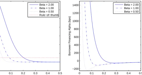
The collateral haircut governs how the cost of capital is adjusted for the lender and the borrower. Panel A of Figure 5 shows the proper schedule of lender financing rates for stocks with various market betas as a function of the collateral haircut. As demonstrated earlier, with a haircut of 25% margin loans are nearly riskfree for stocks with market betas that are not too large. At this collateral level interest rate spreads are under 50 bps even for stocks with a market beta of 2 and under 1 bp for stocks with market beta of 1 and below. As collateral haircuts fall from this level, proper interest rates begin to increase, more rapidly the higher the market beta. This suggests that a borrower facing a lender relying on a rule of thumb margin loan interest rate will have a powerful incentive to negotiate slightly lower collateral haircuts, especially for high beta securities. Panel B of Figure 5 demonstrates this effect by plotting the borrower’s financing alpha (difference between the expected return under the lender’s rule of thumb interest rate of 25 bps and the proper cost of capital) as a function of collateral. A very small reduction in the collateral haircut creates a huge financing benefit for the borrower when holding high market beta securities.

Finally, we examine the effect of changes in volatility. All of the analyses so far have relied on market volatility of 15%. As volatility changes, the crash distribution is altered. While the crash frequency is assumed to be constant, higher volatility increases the crash size since we assume that crashes are constant in Z-scores. We construct a proper schedule of margin loan interest rates as a function of volatility, holding collateral haircuts constant (Panel A of Figure 6). With Reg T haircuts, the margin loans remain quite safe for the lender as annualized daily volatility increases to 50%. With lower collateral haircuts the proper margin loan interest rates climb significantly with volatility. We also calculate the schedule of proper required haircuts, holding margin loan interest rates constant (Panel B of Figure 6). This highlights the dependence of the interest rate/collateral haircut pair on volatility and may partially explain why interest rates and haircuts increased across the board throughout 2008.

3.2 Corporate bonds and structured collateral

In this section we consider the cost of financing the purchase of corporate bonds and corporate asset-backed CDO tranches. In order to characterize the crash consequence functions, B(x), for these two

collateral types we require a valuation model that allows us to describe security values as a function of the crash size, x. To do this we use a modified version of Merton’s (1974) structural model of credit, which includes a common, market factor driving asset returns of various firms, introduced in Coval, Jurek, and Stafford (2009a). This framework will allow us to compute the state-contingent payoffs for bonds, bond indices, and CDO tranches, P(m, x), as a function of the level of the market index at maturity, m, before and after a crash of size,x. To complete valuation we also require a set of Arrow-Debreu prices (Arrow (1964), Arrow-Debreu (1959)) in the pre- and post-crash states,A(m, x), against which the state-contingent payoffs will be integrated. The crash consequence function,B(x), is then simply the

change in the asset value resulting from a market crash,x:

B(x) = Z Pi(m, x)· A(m, x)·dm− Z Pi(m, x= 0)· A(m, x= 0)·dm (27) 3.2.1 State prices

Coval, Jurek, and Stafford (2009a) compute a new set of state-prices for each day in their sample by fitting implied volatilities on five-year equity index options. Their approach produces an expression that adjusts the standard formula for Arrow-Debreu state prices (Breeden and Litzenberger (1978)) for the existence of a implied volatility skew. Because our focus here is not a time-series analysis of the pricing of structured products we will simplify the computation of Arrow-Debreu prices by using the formula of Breeden and Litzenberger (1978). Given a market volatility, σm(x = 0), state-prices corresponding to

each terminal value of the equity index can be computed from:

A(mτ, x) = e−rf·τ_·d 2 σm(x)· √ T·em τ (28) where: d1 = −mτ +σm(x) 2 2 ·τ σm(x)· √ τ and d2 =d1−σm(x)· √ τ (29)

To simplify notation, we have also defined the log moneyness,mτ, as the natural logarithm of the ratio

of the terminal market index level, MT, to the time t futures price, Mt·exp ((rf−δm)·τ). rf is the

we set τ = 5 years, matching the maturity of the Dow Jones North American Investment Grade Index,

rf = 2.5% andδm = 1.5%.

We also need a set of state prices that prevail following a crash of size, x. Since state prices are parameterized by the level of market volatility, σm(x), this requires taking a stand on the post-crash

level of option-implied volatilities. To maintain parsimony we assume that option-implied volatilities exhibit a constant elasticity relative to the log index return (crash), such that the post-crash volatility is given by:

σm(x) = σm(x= 0)·exp (ζ·log(1−x)) (30)

Since the bonds and tranches we examine have maturities of approximately five years, we are interested in estimates of the elasticity, ˆζ, of the five-year option-implied volatilities, rather than a short-dated measure of implied volatility, such as the CBOE VIX index. Using weekly data from January 2003 through June 2009, we estimate the elasticity of the 5year atthemoney option implied volatility to be -0.37 (t-stat: -7.63). By comparison, the elasticity of the VIX index – which is based on short-dated equity index options – is -2.86 (t-stat: -17.61).6 _{In the empirical applications we set the elasticity parameter,} ζ, equal to -0.40, and σm(x = 0) equal to the five year option-implied volatility corresponding to each

day. Whenever objective measures of long-dated volatility are required, we scale the option-implied volatilities by 80% to remove the effect of the volatility risk premium.

3.2.2 State-contingent payoffs

To derive state-contingent asset payoffs, as a function of the aggregate equity index level, we modify Merton’s (1974) structural model of credit to include a common factor driving asset returns of various firms. Each firm is assumed to be characterized by a triple of parameters: the asset beta (βa), the

debt-to-asset ratio (D_A), and idiosyncratic asset volatility (σe). The state-contingent default probabilities

and expected payoffs can then be expressed as a function of the (log) terminal moneyness, mτ. With

τ =T−t periods left until maturity, the state-contingent default probability for an individual bond is then given by:

pD(mτ) = Prob h ˜ AT(mτ)< D i = Φ [−η(mτ)] (31)

6_{Elasticity estimates based on daily data are -0.29 (t-stat: -14.84) for the five-year option implied volatility, and -3.23} (t-stat: -42.54) for the VIX index.

where: η(mτ) = − ln_AD t −(rf ·τ+βa·mτ) σ· √ T , (32)

Conditional on default the terminal asset value – on which the bond recovery is based – can be derived as a function of the terminal moneyness,mτ:

Et h ˜ AT(mτ)|A˜T(mτ)< Di i = At·exp rf·τ+βa·mτ+ 1 2 ·σ 2 ε ·τ ·Φ [−η(mτ)−σε· √ τ] Φ [−η(mτ)] (33)

It is common to assume that a fraction,ν, of the terminal asset value is lost to bankruptcy costs (Leland (1994)). For example, in order to fit the data, Cremers, Driessen, and Maenhout (2009) need bankruptcy costs to be approximately equal to 50% of the terminal asset value. Finally, we can write the expected

state-contingent payoff for an individual bond as:

PBond(mτ) = 1−  1− (1−ν)·Et h ˜ AT(mτ)|A˜T(mτ)< D i D  ·pD(mτ) (34)

Tranches are derivative claims, whose payoffs derive from the value of of the underlying bond portfolio. A tranche is characterized by two attachments points, [X, Y]. The lower attachment,X, point defines the largest portfolio loss that will not impair the tranche payoff; the upper attachment point,Y, describes the portfolios loss at which the tranche value is completely wiped out. In order to derive the state-contingent tranche payoffs we will make a convenient simplification and assume that the underlying portfolio is infinitely diversified (N → ∞), and comprised of identical bonds. The large, homogenous portfolio (LHP) assumption implies that the bond portfolio payoff converges in probability to the expression derived above, and the tranche payoff can be obtained by simply applying the contractual tranche terms to (34): P[X,Y]_(m τ) = 1− 1 Y −X · max(1−X)− PBond_(m τ),0 −max(1−Y)− PBond_(m τ),0 (35)

In our empirical analysis we focus on two assets: AA-rated corporate bonds – the highest rated class on bonds for which there is a reliably broad cross-section of data available – and a [7,10] tranche referencing the Dow Jones North America Investment Grade index (CDX.NA.IG). The CDX.NA.IG index is comprised of the debt of 125 issuers with an average rating between BBB+ and A-, such that only sufficiently senior tranches are expected to garner high credit ratings. Finally, rather than calibrate

new model parameter values for both securities on each day we will use the time-series means reported in Table VI of Coval, Jurek, and Stafford (2009a). In particular, we fix the parameters for a typical AA-rated bond atβa= 0.85, D_A = 0.19, andσe = 0.31; and for the “average” security in the CDX.NA.IG

index at –βa= 0.74, D_A = 0.34, andσe= 0.27.

To compute the state-contingent bond and tranche payoff functions following a crash of magnitudex, we proceed as follows: (1) update the level of aggregate market volatility by using the constant elasticity of volatility specification described earlier; (2) scale the idiosyncratic volatility estimate,σe, by the ratio

of the post-crash market volatility,σm(x), to the baseline volatility (0.15), in order to ensure that asset

betas remain unchanged; and, (3) compute the post-crash debt-to-asset ratio as follows:

D At(x)

= D

A_t−

·exp (−βa·log (1−x)) (36)

The updated state contingent asset payoffs,Pi_{(m, x), are then obtained by applying the formulas, (34)}

and (35), and valuation is completed using the post-crash state prices,A(m, x).

3.2.3 Calibration results

In early 2007, the credit spreads on AAA-rated corporate bonds and the [7, 10] tranche of the CDX.IG were nearly the same. While not formally rated, the [7, 10] tranche was considered by practitioners to be the junior most CDX tranche that would be rated AAA. The similar ratings imply that the unconditional expected losses for these two securities are essentially the same. However, the state-contingent payoff functions for similarly-rated bonds and tranches can be quite different. Panel A of Figure 7 displays the calibrated state-contingent payoff functions for a corporate bond that was rated AA and the [7, 10] tranche of the CDX.NA.IG. The primary way in which these securities differ is that the tranche concentrates its losses in worse economic states. A consequence of this state-contingent profile is that the drop in expected payoff as economic conditions deteriorate is steeper and approaches with a smaller shock. Therefore, the quality of the tranche as collateral against crashes is inferior to that of the bond. For example, holding the haircut constant, the crash size that exhausts the collateral is always smaller for this tranche than for the bond. Similarly, the necessary haircut for the lender to be protected against a crash of sizexis always larger for this tranche than for the bond, as illustrated in Panel B of Figure 7. The different crash exposures between these two similarly-rated securities suggest that the proper schedules of collateral haircuts/financing spreads should be different. These differences should be espe-cially acute when financing spreads are very low or when haircuts are very low. Panel C of Figure 7 plots the proper financing spread as a function of collateral haircut for the bond and tranche. With relatively

high collateral levels, the margin loans supporting both the bond and tranche are close to riskfree, com-manding negligible financing spreads. Even with very low collateral levels, the margin loan supporting the bond is nearly riskfree. However, the margin loan supporting the tranche becomes considerably more risky at low collateral haircuts and should command a noticably higher financing spread.

To the extent that the financing spreads for tranches are set based on the proper spreads for similarly-rated bonds (i.e. much too low when haircuts are small) the investor in the tranche receives a highly valuable financing benefit. As we did earlier, we calculate the borrower’s financing alpha as the difference between the borrower’s expected return under the lender’s imperfect financing rule and the proper cost of capital. The lender’s rule of thumb rule is to charge a single financing spread to both bond and tranche investors based on the proper financing spread for a bond with a haircut of 10%. Panel D in Figure 7 shows the magnitude of the borrower’s financing alpha as a function of collateral. For very low collateral haircuts, the borrower’s expected return due to this financing benefit becomes enormous.

4

Model Implications

The contribution of this paper is to highlight how differences in systematic risk exposures and vari-ation in the aggregate quantity of risk, can combine to produce extreme changes in the crash risk cost of capital for a variety of common security types, and consequently to spreads and haircuts associated with collateralized loans against these securities. These effects manifest themselves even in the absence of asymmetric information, liquidity costs, agency concerns, or time-varying risk aversion.

Within our framework, every financing contract is characterized by a haircut, H, and a fee, ξl (or

interest rate) that has to be remitted to the lender in order to compensate him for bearing losses in excess of the haircut. As the haircut is varied, the lending rate (or spread over the riskfree rate) adjusts to reflect differences in risk-sharing, producing a schedule of haircut-spread pairs between which the agents are indifferent at initiation of the loan. As the aggregate quantity of risk – the state variable – changes over time, this financing agreement has to be renegotiated. In financial markets, renegotiation can be accomplished relatively easily, as most collateralized lending is overnight. Although borrowers can select from a continuum of new haircut-spread pairs, in practice, there seems to be significant interest in contracts that do not require significantex post adjustments to the financing terms as market conditions change. For example, Gorton and Metrick (2009) interpret the large rise in haircuts for structured securities during the 2007-2008 credit crisis as a panicked “run on repo,” suggesting that haircut stability is of central importance to market practitioners. This raises the question of what constitutes “good” collateral, and what is necessary to ensure the stability of spreads and haircuts?

4.1 Stress tests

Our analytical framework enables us to explore how the financing terms for various types of securities are expected to adjust in response to changes in the level of the state variables controlling the distribution of aggregate jump sizes and their pricing. In the model, these variables are the aggregate volatility and risk aversion (assumed to be constant). We consider two polar “stress test” scenarios: in the first, the haircut is held fixed, and the spread is allowed to vary; in the second, the spread is held fixed, and the haircut adjusts. To the extent that market participants wish to keep spreads low and stable, this exercise can be used to pin down the minimal necessary haircut (e.g. to keep spreads below 50bps across the desired state variable range).

The simplest conceivable financing arrangement occurs when the maximum crash size is bounded at

x∗. If the haircut is fixed at any value greater than or equal to B(x∗), the lender’s sensitivity is equal to zero (i.e. he bears no risk). Portfolio margin or risk-based margin rules can be viewed as operating in this way. For example, under portfolio margining the required haircut is assigned to all assets within a class based on the losses expected in the event of an underlying price move of ±y%, where y is determined based on the maximum of an absolute return shock and the return associated with some critical Z-score value.7 More generally, when the crash magnitude is not bounded, the lender is exposed to the risk of loss, for which he charges a spread depending on the posted haircut.

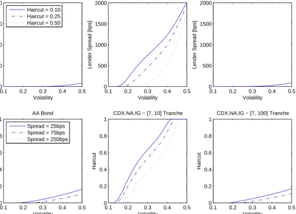
In Figure 8 we report the results of a stress test conducted on the AA-rated bond and the [7, 10] CDX.NA.IG tranche described earlier, as well as for a hypothetical [7, 100] CDX.NA.IG tranche. The first row of the figure plots the proper financing spreads at three different haircut levels, while the second row shows the proper haircuts at three different financing spreads, all as a function of current annualized stock market volatility. There are two important messages from this analysis. First, the bond represents good collateral, while the equivalently rated [7, 10] tranche does not. In fact, the [7, 10] tranche is

expected to require a 100% haircut when volatility exceeds approximately 40%. Second, the hypothetical [7, 100] CDX.NA.IG tranche would be good collateral.

The analysis also highlights that reliance on credit ratings as a basis for collateral haircuts is prob-lematic, if it is desirable to have stable spreads across economic conditions. While both of the securities in the previous analysis would haveex antereceived a rating of AA, they exhibit very different financing term dynamics. Credit ratings encourage simplified imperfect collateral haircut/spread schedules that are likely to implicitly assume that all securities within a rating category share similar crash exposures.

7_{This approach parallels the intuition of portfolio value-at-risk computations. For example, under a Gaussian} distribu-tion, the 99.99% VaR corresponds to a critical Z-score value of -3.72. For index options, typical broker rules are based on the maximum of an underlying price moveyof +6%/-8%, and the return implied by a critical Z-score value of -5.

As emphasized by Coval, Jurek, and Stafford (2009b), credit ratings do not focus on state-contingent risk profiles. As we demonstrated above, the expected recovery value conditional on a market crash can be highly time varying and meaningfully different across similarly-rated securities.

4.2 Financing terms during the credit crisis

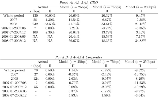
Gorton and Metrick (2009) report some statistics on average repo rates and haircuts for a wide range of securities throughout the financial crisis applicable for dealers. Despite their name, the broker-dealers were functionally the investors in these securities who largely financed themselves in the repo market. Table 2 compares the repo spreads and haircuts for AAA-rated CDOs and corporate bonds, as reported in Gorton and Metrick (2009), to our model-implied funding schedule. In the first-half of 2007, AAA-rated CDO tranches had a collateral haircut of 0% and a financing spread of 7 bps. This is clearly inconsistent with the model. With no haircut, the financier is bearing the crash risk and should be collecting the full crash risk premium. For many highly-rated CDO tranches, the unlevered annualized crash risk premium was large. For instance, according to this analysis the [7, 10] CDX.NA.IG tranche should have earned an average crash risk premium of 82 bps over the first half of 2007. The repo market’s funding schedule in the pre-crisis period helps reconcile the view that some of the highly-rated CDO tranches were simultaneously overvalued and kept on the balance sheets of the broker-dealers. The transaction alpha of selling the overpriced securities was considerably smaller than the financing alpha available by holding on to them.

In the second half of 2007, collateral haircuts on AAA-rated CDO tranches averaged 8.3% and the associated financing spreads averaged 108 bps, according to Gorton and Metrick (2009). In 2008, hair-cuts for these securities averaged 53.5% with average financing spreads of 232 bps. The large increases in haircuts and financing spreads suggest that the effective financing rule used in repo markets is a function of market volatility, consistent with the predictions of our framework. We can illustrate how the signif-icant increase in volatility over this period translates into model-implied haircuts/spreads for the bond and tranche described earlier. Specifically, we construct a proper schedule of collateral haircuts/margin loan spreads as a function of volatility (0.8 x VIX). In Figure 9, we plot the time series of the minimum required haircuts for the bond and tranche from 2007 through 2009 for a lender charging a constant financing spread of either 25 bps or 250 bps. With a financing spread of 25 bps, the proper haircut for the bond never exceeds 20%, while the proper haircut for the tranche rises from an initial level near zero, peaking over 100% at the height of the crisis.

4.3 Robust repo collateral

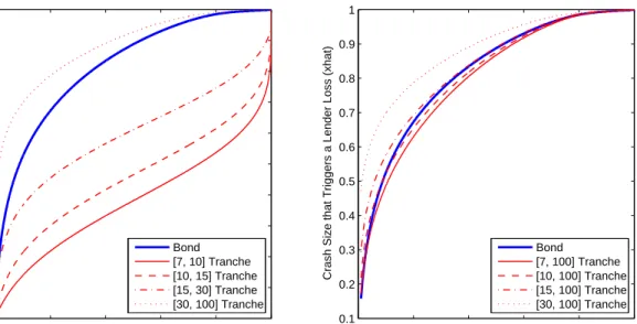
We can develop intuition for the safety of a collateralized loan from the approximation of the lender’s dollar charge (11). This formula highlights that the slope of the crash consequence function around the index level at which the lender sustains losses, ˆx, plays a key role in determining the level – and dynamics through time varying volatility – of borrowing rates. For equities, this slope can be linked to equity betas, which typically range between 0 and 2; although in principle, stocks with higher betas could be created. For credit instruments, the market practice has been to link this exposure to credit ratings. However, as demonstrated in Coval, Jurek, and Stafford (2009a) the systematic risk profiles of similarly-rated securities can be quite different. Unlike highly-rated corporate bonds, for which the sensitivity, B0(ˆx), is modest due to the the typically high recovery values, the slope can be very large for many types of structured finance securities. Figure 10 plots the crash sizes at which haircuts are exhausted (ˆx) for the tranches of the CDX.NA.IG that were considered equivalent to being AAA-rated. Only the [30, 100] tranche has lower crash exposure than the underlying asset pool. With small haircuts, the mezzanine tranches shift much of the crash risk onto the lender. This translates into dramatically different spread/haircut dynamics when these securities are used as collateral.

Figure 10 also plots the crash sizes at which haircuts are exhausted for various hypothetical senior tranches. All of these represent good collateral. Because, in practice, many tranches were constructed to be relatively thin (e.g. [7, 10] instead of [7, 100]), the rate at which the lender incurs losses after the borrower haircut is exhausted is extremely fast. Put differently, in order to ensure stable spreads when these types of structured securities are used as collateral, haircuts must be significantly larger than for identically rated bonds. Another alternative is to make tranches wider to ensure that the rate at which the lender’s loss given default grows with the crash size is mitigated.

Most of the securities for which large swing in haircuts were observed during the credit crisis of 2007-2008 – AAA RMBS/CMBS, subprime MBS, CLOs, and CDOs – have crash consequence functions that are very steep around modest crashes, i.e. low recovery values in the event of a crash. As such, the large increase in haircuts is not surprising when viewed from the perspective of our framework, given the large concurrent increases in equity market volatility. In particular, we have shown that highly-rated mezzanine tranches of a CDO consisting of investment grade corporate bonds are poor collateral, because there is a real chance they will loseall of their value in a crash. Resecuritizing these tranches in a second-generation CDO does not resolve this issue; a super-senior [30, 100] tranche of a re-securitized pool of [7, 10] mezzanine tranches on investment grade corporate bonds, would be poor collateral for the same reason. However, the stability of spreads/haircuts can be increased considerably by increasing the

tranche width. A [7, 100] tranche could in fact be financed with a stable haircut and spread during this period, precisely because its recovery value in the event of a crash remains high.

It is generally hard to find corporate bonds with very low expected recovery values and a high probability of default. If these were to exist, they would likely have a systematic risk profile somewhat similar to a mezzanine CDO tranche, where a modest economic downturn eliminates their entire value. Even a super-senior tranche of a CDO with these types of bonds would represent poor collateral as the entire asset pool can go to zero. While corporate bonds of this type do not exist, subprime mortgages share many of these qualities. Highly levered home borrowing, limited prospects of paying off the loan without continued house price appreciation, and generally large costs associated with liquidating real estate collateral, combine to produce rapidly declining values as a function of aggregate economic conditions. Moreover, since these loans tended to be issued in areas with relatively high price-to-rent ratios, convergence to average price-to-rent ratios would further adversely affect the recovery value in default (Las Vegas, Florida, and California). As a result, subprime mortgages exhibit the central feature of unstable collateral – a steeply sloped crash consequence function even in the vicinity of small economic shocks. Securitizations of these products (e.g. RMBS, or CDOs of subprime RMBS) inherit these systematic risk profiles, and would also be expected to constitute unstable collateral.

4.4 State-contingent adverse selection

The striking change in repo market financing terms over the course of the credit crisis has been attributed to an increase in the “information sensitivity” of the collateral typically debt instruments -which spurred concerns about adverse selection (Holmstr¨om (2008), Gorton and Metrick (2009), Dang, Holmstr¨om, and Gorton (2010)). These authors argue that following the initial deterioration in macroe-conomic conditions, an increased incentive to produce information led to a large decline in trade, or a “run on repo.” This interpretation is based on the premise that the majority of the relevant state-contingent uncertainty is idiosyncratic, and in such a setting, information asymmetry creates the potential for ad-verse selection. However, the focus on idiosyncratic risks is more appropriate in a firm-level security analysis, rather than for the diversified pools of assets (ABX, CDX), and derivatives thereon (CDO, CDO-squared), that were at the center of the crisis. In the limit of complete diversification (e.g. an index), there is no value to private information gathering and adverse selection plays no role (Sub-rahmanyam (1991), Gorton and Pennacchi (1993)). In this case, the only remaining component is the state-contingent mean payoff profile of the asset class (Figure 7; top left panel), reflecting its fundamental (or systematic) risk exposure. Without explicitly accounting