Modelling of Spatial Effects in Count Data
A thesis submitted by
Stephanie Glaser
to attain the degree of
Doctor oeconomiae (Dr. oec.)
Faculty of Business, Economics and Social Science
Institute of Economics
Chair of Econometrics and Statistics
Stuttgart-Hohenheim
2017
Doktors der Wirtschaftswissenschaften (Dr. oec.) angenommen.
Datum der Disputation: 7. M¨arz 2017
Dekan: Prof. Dr. Dirk Hachmeister
Pr¨ufungsvorsitz: Prof. Dr. Katja Schimmelpfeng Erstgutachter: Prof. Dr. Robert Jung
1 Introduction 10
1.1 Motivation . . . 10
1.2 Introduction to Spatial Econometric Modelling . . . 13
2 Literature on Spatial Econometric Models for Count Data 19 2.1 Introduction . . . 19
2.2 Spatially Lagged Covariates Models . . . 20
2.3 Spatial Error Models . . . 21
2.4 Spatial Autocorrelation Models . . . 23
3 Investigation and Extension of the Poisson SAR Model 31 3.1 Introduction . . . 31
3.2 The Poisson Autoregressive Model and Limited Information Likelihood Esti-mation . . . 31
3.3 Extensions of the Poisson SAR Model . . . 33
3.4 Monte Carlo Study . . . 36
3.4.1 Data Generating Processes and Study Setup . . . 36
3.4.2 Monte Carlo Parameter Estimates . . . 37
3.4.3 Monte Carlo Estimates of Marginal Effects . . . 43
3.5 Model Selection: Scoring Rules . . . 48
3.6 Empirical Application: Start-up Firm Births . . . 49
3.6.1 Data . . . 49
3.6.2 Empirical Results . . . 52
3.7 Summary . . . 55
4 The Spatial Linear Feedback Model 57 4.1 Introduction . . . 57
4.2 Modelling Approach . . . 58
4.3 Diagnostics . . . 60
4.4 Monte Carlo Study . . . 62
4.4.1 Data Generating Process and Study Setup . . . 62
4.4.2 Monte Carlo Results . . . 63
4.5 Empirical Application: Start-up Firm Births . . . 71
4.6 Unilateral Modelling with Composite Maximum Likelihood . . . 77
4.7 Summary . . . 78
5 Spatial Panel Models: Forecasting Crime Counts 79 5.1 Introduction . . . 79
5.2 Data: Crime in Pittsburgh . . . 79
5.3 The Spatial Linear Feedback Panel Model with Fixed Effects . . . 82
5.3.1 Specification of the Spatial Linear Feedback Panel Model . . . 82
5.4 A Dynamic Spatial Panel Model for Counts with Multiplicative Fixed Effects 87
5.4.1 Specification of the Model with Multiplicative Fixed Effects . . . 87
5.4.2 Quasi-Differenced GMM Estimation . . . 88
5.4.3 Illustration with Simulated Data . . . 90
5.4.4 Empirical Application: Forecasts for Pittsburgh’s Crime Counts . . . 93
5.5 A Dynamic Spatial Panel Model for Counts with Additive Fixed Effects . . . 95
5.5.1 Specification of the Model with Additive Fixed Effects . . . 95
5.5.2 System GMM Estimation . . . 96
5.5.3 Illustration with Simulated Data . . . 98
5.5.4 Empirical Application: Forecasts for Pittsburgh’s Crime Counts . . . 101
5.6 Summary . . . 104
6 Conclusion 105 A Further Results for the SAR Models 108 A.1 Monte Carlo Parameter Estimates . . . 108
A.2 Monte Carlo Marginal Effects Estimates . . . 123
A.3 Descriptives of the Start-Up Firm Birth Data Set . . . 138
A.4 Empirical Results for SAR Models . . . 139
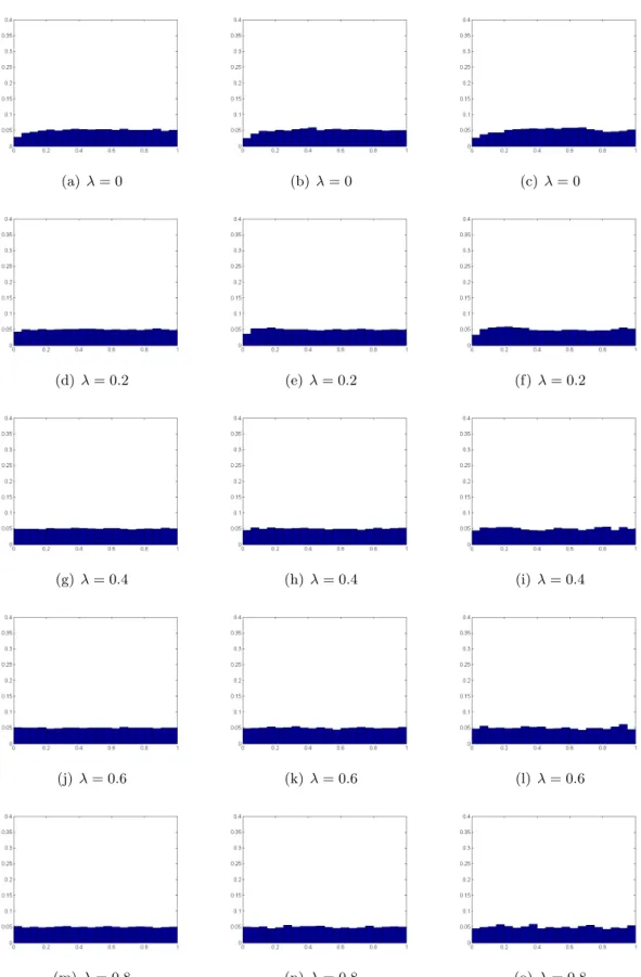
B Further Results for the SLF Models 145 B.1 Monte Carlo Results for PIT Histograms . . . 145
B.2 Monte Carlo Parameter Estimates . . . 148
B.3 Empirical Results for SLF Models . . . 150
C Further Results for the Panel Models 151 C.1 Empirical Results for the P-SLFP Model . . . 151
C.2 Empirical Results for the Dynamic Panel Model with Multiplicative Fixed Effects . . . 155
C.3 Empirical Results for the Dynamic Panel Model with Additive Fixed Effects . . . 157
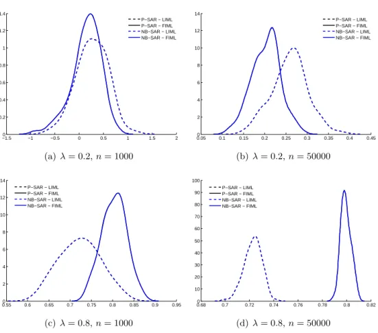
1 Stylized patterns of spatial correlation . . . 13 2 Components of the spatial autoregressive effect . . . 18 3 Extensions of the P-SAR model . . . 35 4 Monte Carlo results of probability density estimates for ˆλof generated P-SAR
data . . . 37 5 Monte Carlo results of probability density estimates for ˆλ of generated
NB-SAR data, α= 1/8 . . . 39 6 Monte Carlo results of probability density estimates for ˆλ of generated
NB-SAR data, α= 1/2 . . . 40 7 Heat maps for the relative bias of estimated median direct marginal effects
for all generated data sets . . . 44 8 Heat maps for the relative bias of estimated median total marginal effects for
all generated data sets . . . 45 9 Map of observations for subirthin deciles . . . 49 10 Histogram of start-up firm birth counts . . . 51 11 Predicted probabilities of P-SAR, ZIP-SAR, NB-SAR for the start-up firm
births data . . . 54 12 PIT histograms for Monte Carlo estimates from the NB-SLFM . . . 67 13 Estimated conditional expectations of the number of start-up firm births . . . 73 14 Nonrandomized PIT histograms for SLF models and the start-up firm births
data . . . 74 15 Relative deviations plot for SLF models and the start-up firm births data . . 75 16 Map of time averages of Part I crimes in Pittsburgh . . . 80 17 Pittsburgh crime data descriptives . . . 82 18 Scoring rules of density forecasts from the P-SLFPM for the Pittsburgh crime
data . . . 84 19 Nonrandomized PIT histograms of density forecasts from the P-SLFPM for
the Pittsburgh crime data . . . 86 20 PIT histograms of Monte Carlo results for P-SLFM . . . 146 21 PIT histograms of Monte Carlo results for NB-SLFM estimated with P-SLFM 147
1 SAR models Monte Carlo setup . . . 37
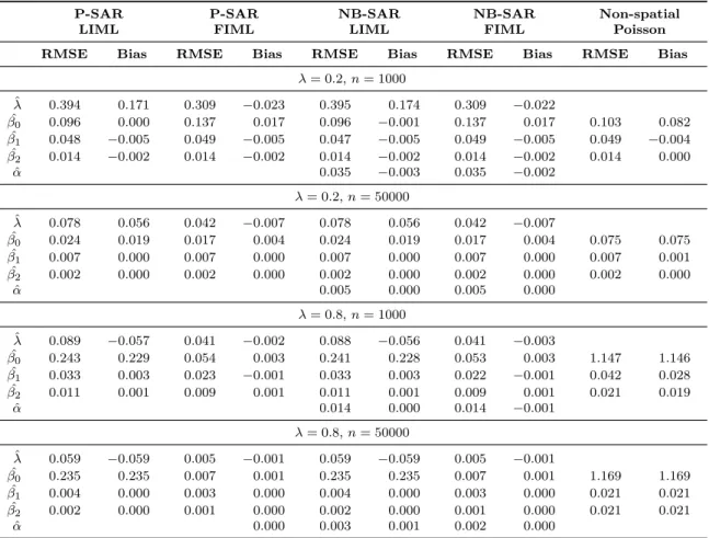
2 Monte Carlo results of parameter estimates for generated P-SAR data with λ={0.2,0.8} andn={1000,50000} . . . 38
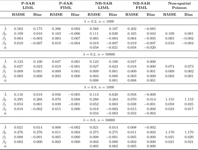
3 Monte Carlo results of parameter estimates for generated NB-SAR data with α= 1/8,λ={0.2,0.8}and n={1000,50000} . . . 41
4 Monte Carlo results of parameter estimates for generated NB-SAR data with α= 1/2,λ={0.2,0.8}and n={1000,50000} . . . 42
5 Monte Carlo results of median marginal effects for P-SAR Data,λ={0.2,0.8}, n={1000,50000} . . . 46
6 Monte Carlo results of median marginal effects for NB-SAR data,λ={0.2,0.8}, n={1000,50000},α= 1/8 . . . 47
7 Monte Carlo results of median marginal effects for NB-SAR data,λ={0.2,0.8}, n={1000,50000},α= 1/2 . . . 47
8 Description of start-up firm births data . . . 50
9 Number of neighbors in different spatial weight matrices for the start-up firm births data . . . 51
10 Estimation results forλfrom SAR models for the start-up firm births data . 52 11 Scoring rules of SAR model estimates for the start-up firm births data . . . . 53
12 Median marginal effects of P-SAR, NB-SAR, ZIP-SAR for the start-up firm births data with weight matrixWdnn . . . 56
13 Monte Carlo results for P-SLFM . . . 63
14 Monte Carlo results for NB-SLFM . . . 64
15 Monte Carlo results of median marginal effects for P-SLFM data . . . 65
16 Monte Carlo results of median marginal effects for NB-SLFM data . . . 66
17 Monte Carlo results for NB-SLFM, α= 0.5 . . . 68
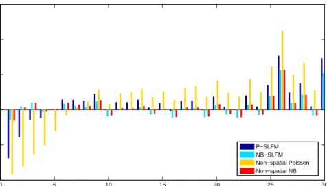
18 Monte Carlo results for NB-SLFM data estimated with P-SLFM model,α= 0.2 69 19 Estimation results from P-SLF, NB-SLF, non-spatial Poisson, non-spatial NB models for the start-up firm births data . . . 72
20 Median marginal effects of P-SLFM, NB-SLFM, non-spatial Poisson, and non-spatial NB for the start-up firm births data with weight matrix Wdnn . . 76
21 Estimation results of the unilateral modelling approach using P-SLFM for the start-up firm births data . . . 78
22 Descriptive statistics of the Pittsburgh crime data set . . . 81
23 Results from the P-SLFPM for the Pittsburgh crime data . . . 85
24 Monte Carlo results for the dynamic spatial panel model with multiplicative fixed effects . . . 92
25 Results from the dynamic spatial panel model with multiplicative fixed effects for the Pittsburgh crime data . . . 94
26 Monte Carlo results for the dynamic non-linear spatial panel model with additive fixed effects . . . 99
27 Monte Carlo results for the dynamic linear spatial panel model with additive fixed effects . . . 100 28 Results from the dynamic non-linear spatial panel model with additive fixed
effects for the Pittsburgh crime data . . . 102 29 Results from the dynamic linear spatial panel model with additive fixed effects
for the Pittsburgh crime data . . . 103 30 Monte Carlo results of parameter estimates for FIML estimations of P-SAR
data and P-SAR model . . . 108 31 Monte Carlo results of parameter estimates for LIML estimations of P-SAR
data and P-SAR model . . . 109 32 Monte Carlo results of parameter estimates for FIML estimations of P-SAR
data and NB-SAR model . . . 110 33 Monte Carlo results of parameter estimates for LIML estimations of P-SAR
data and NB-SAR model . . . 111 34 Monte Carlo results of parameter estimates for QML estimations of P-SAR
data and non-spatial Poisson model . . . 112 35 Monte Carlo results of parameter estimates for FIML estimations of NB-SAR
data (α= 1/8) and P-SAR model . . . 113 36 Monte Carlo results of parameter estimates for LIML estimations of NB-SAR
data (α= 1/8) and P-SAR model . . . 114 37 Monte Carlo results of parameter estimates for FIML estimations of NB-SAR
data (α= 1/8) and NB-SAR model . . . 115 38 Monte Carlo results of parameter estimates for LIML estimations of NB-SAR
data (α= 1/8) and NB-SAR model . . . 116 39 Monte Carlo results of parameter estimates for QML estimations of NB-SAR
data (α= 1/8) and non-spatial Poisson model . . . 117 40 Monte Carlo results of parameter estimates for FIML estimations of NB-SAR
data (α= 1/2) and P-SAR model . . . 118 41 Monte Carlo results of parameter estimates for LIML estimations of NB-SAR
data (α= 1/2) and P-SAR model . . . 119 42 Monte Carlo results of parameter estimates for FIML estimations of NB-SAR
data (α= 1/2) and NB-SAR model . . . 120 43 Monte Carlo results of parameter estimates for LIML estimations of NB-SAR
data (α= 1/2) and NB-SAR model . . . 121 44 Monte Carlo results of parameter estimates for QML estimations of NB-SAR
data (α= 1/2) and non-spatial Poisson model . . . 122 45 Monte Carlo results of marginal effects for FIML estimations of P-SAR data
and P-SAR model . . . 123 46 Monte Carlo results of marginal effects for LIML estimations of P-SAR data
and P-SAR model . . . 124 47 Monte Carlo results of marginal effects for FIML estimations of P-SAR data
48 Monte Carlo results of marginal effects for LIML estimations of P-SAR data
and NB-SAR model . . . 126
49 Monte Carlo results of marginal effects for QML estimations of P-SAR data and non-spatial Poisson model . . . 127
50 Monte Carlo results of marginal effects for FIML estimations of NB-SAR data (α= 1/8) and P-SAR model . . . 128
51 Monte Carlo results of marginal effects for LIML estimations of NB-SAR data (α= 1/8) and P-SAR model . . . 129
52 Monte Carlo results of marginal effects for FIML estimations of NB-SAR data (α= 1/8) and NB-SAR model . . . 130
53 Monte Carlo results of marginal effects for LIML estimations of NB-SAR data (α= 1/8) and NB-SAR model . . . 131
54 Monte Carlo results of marginal effects for QML estimations of NB-SAR data (α= 1/8) and non-spatial Poisson model . . . 132
55 Monte Carlo results of marginal effects for FIML estimations of NB-SAR data (α= 1/2) and P-SAR model . . . 133
56 Monte Carlo results of marginal effects for LIML estimations of NB-SAR data (α= 1/2) and P-SAR model . . . 134
57 Monte Carlo results of marginal effects for FIML estimations of NB-SAR data (α= 1/2) and NB-SAR model . . . 135
58 Monte Carlo results of marginal effects for LIML estimations of NB-SAR data (α= 1/2) and NB-SAR model . . . 136
59 Monte Carlo results of marginal effects for QML estimations of NB-SAR data (α= 1/2) and non-spatial Poisson model . . . 137
60 Descriptives of start-up firm births data set . . . 138
61 P-SAR estimates for the start-up firm births data set . . . 139
62 NB-SAR estimates for the start-up firm births data set . . . 140
63 ZIP-SAR estimates for the start-up firm births data set . . . 141
64 HP-SAR estimates for the start-up firm births data set . . . 142
65 Median marginal effects of P-SAR, NB-SAR, ZIP-SAR for the start-up firm births data set with weight matrix Wcon . . . 143
66 Median marginal effects of P-SAR, NB-SAR, ZIP-SAR for the start-up firm births data set with weight matrix Wnn . . . 144
67 Monte Carlo results for P-SLFM data with a contiguity matrix . . . 148
68 Monte Carlo results for P-SLFM data withβ = (1.5,1.5,1.5) . . . 149
69 Estimation results from P-SLF and NB-SLF for the start-up firm births data set with weight matricesWcon and Wnn . . . 150
70 Estimation results from the P-SLFPM with summer dummy for the Pitts-burgh crime data . . . 151
71 Point forecast evaluation of P-SLFPM with summer dummy for the Pitts-burgh crime data . . . 151
72 Scoring rules of density forecasts from P-SLFPM with summer dummy for the Pittsburgh crime data . . . 152
73 Point forecast evaluation of P-SLFPM for the Pittsburgh crime data . . . 153 74 Scoring rules of density forecasts from P-SLFPM for the Pittsburgh crime data154 75 Estimation results from the multiplicative fixed effects model with summer
dummy for the Pittsburgh crime data . . . 155 76 Point forecast evaluation of the multiplicative fixed effects model with summer
dummy for the Pittsburgh crime data . . . 155 77 Point forecast evaluation of the multiplicative fixed effects model for the
Pitts-burgh crime data . . . 156 78 Estimation results from the non-linear additive fixed effects model with
sum-mer dummy for the Pittsburgh crime data . . . 157 79 Point forecast evaluation of the non-linear additive fixed effects models with
summer dummy for the Pittsburgh crime data . . . 157 80 Estimation results from the linear additive fixed effects model with summer
dummy for the Pittsburgh crime data . . . 158 81 Point forecast evaluation of the linear additive fixed effects model with
sum-mer dummy for the Pittsburgh crime data . . . 158 82 Point forecast evaluation of the non-linear additive fixed effects model for the
Pittsburgh crime data . . . 159 83 Point forecast evaluation of the linear additive fixed effects model for the
1.1 Motivation
Methods of spatial statistics have been widely applied in fields like biometrics and geostatis-tics after Whittle (1954) introduced the first spatial models. Spatial econometrics, however, has only been studied for the past 40 years. Paelinck and Klaassen (1979) published the first work which deals solely with this sub-discipline of econometrics. The characteristic property of spatial data in contrast to non-spatial data is that it links attributes to a geographic lo-cation (Fischer and Wang, 2011).1 In case of a space-time data set information about time is included, too. Due to this additional information, it is possible to model dependencies between different observations which rely on geographical proximity. A similar concept in non-spatial modelling can only be found with regard to the time dimension. Hence, many concepts of spatial models have been inspired by the time series literature. Unfortunately, an essential property of time series does not hold in spatial modelling: Whereas time series have a natural ordering along the time line – from the oldest to the most recent observa-tion – spatial data form a network which does not have a defined starting and end point. Concepts like predetermination, which often facilitates estimation in the time series context, generally do not exist in spatial modelling. Tobler’s first law of geography summarizes this circumstance nicely: “everything is related to everything else, but near things are more re-lated than distant things” (Tobler, 1970, p. 236). It also highlights another key assumption of spatial modelling: While it is anticipated that everything, for example every county or census tract, is connected to the other units through the spatial process, it is also assumed that this connection depends on the proximity of units, i.e. is diminishing with increasing distance.
The use of spatial models can either be motivated from a theoretical or practical viewpoint. In practice, data may show peculiar properties, e.g. spatial heterogeneity, that make the use of a spatial model specification advisable. From a theoretical perspective, spatial mod-els can help to formalize the relations between agents which interact in such a way that aggregate patterns are observable (Anselin, 2002). Different reasons can be thought of why a spatial autoregressive structure might exist in the data at hand and why it should be modelled: First of all, one might originally be interested in modelling the interactions of agents or their reactions on previous decisions of neighbors which depend on the proximity (of geographic or other nature) to each other, e.g. trade flows. This can be accomplished by using panel data (often called space-time data) but also cross-sectional data can contain such dependencies. The observed state in a cross-section represents an equilibrium which has been constituted by iterative actions and reactions of neighboring units. But even if the actual research question does not suggest a spatial dependency in the data, it can be introduced by missing covariates. For example, if the outcome of these missing covariates is identical for several units, which are part of the same larger scale region, neglecting them
1
This definition reflects the basic understanding of spatial data. In econometric modelling the geographic information is sometimes replaced by a different proximity measure, e.g. by technological proximity of industry sectors (Abdelmoula and Bresson, 2005, 2007).
will impose a positive spatial dependency on the dependent variable for which the actually included regressors do not account for. An empirical example for this is provided by Bhat et al. (2014) who suppose that the unobserved overall perceptions regarding the profitability of potential location decisions are similar for neighboring units, if they are defined on a small scale, since the perceptions apply to a larger region. LeSage and Pace (2009, pp. 25) of-fer a comprehensive discussion of these and other motivational aspects for spatial modelling.
Spatial econometrics as an own sub-discipline has borrowed much from spatial statistics, but still it focusses on different aspects of spatial processes. Spatial statistics (which is em-ployed in fields like Biostatistics, Ecology, or Geography) is mostly interested in visualizing the spatial structure within the data (Kauermann et al., 2012). Therefore, formalized models containing non-spatial covariates are rarely used and estimation methods are strongly driven by their application. Spatial econometrics in contrast addresses two features of spatial data – spatial dependence between observations and spatial heterogeneity, i.e. “place-to-place” non-constant variance (Griffith and Paelinck, 2007). The focus often lies on estimating the size of spillover effects (Kauermann et al., 2012) usually in combination with effects of ex-planatory variables. This coincides with the scope of this thesis: The central purpose is to develop original count data models for spatial data which excludes models with log trans-formed counts or rates of counts as the dependent variable. These models need to estimate a (global) spatial effect, which allows that changes in the observation of one geographical unit potentially affect the outcomes of all other units. Additionally, the model must allow for explanatory variables aside the spatial terms which is a standard in econometric modelling.
A large variety of techniques have evolved in spatial econometrics, most of them for the modelling of continuous spatial data, but also other data types are considered. But still, the modelling of spatial count data, i.e. data which consists of non-negative integers, is in its infancy, with some propositions but few established methods. While spatial heterogeneity is included into count data models on a regular basis, spatial autoregression of the dependent variable is rarely addressed in count data applications so far. Seemingly, the only well estab-lished modelling strategy, which has been transferred from spatial statistics, is the modelling of a spatially correlated error term using a conditional autoregressive (CAR) scheme. There, the errors conditional on their neighbors are assumed to be normally distributed. However, this only induces a spatial structure in the error term, not in the observations, regarding it as a nuisance. Aside from that, the special structure of count data models has hindered the direct transfer of the model structure for continuous spatial data. Instead of spatially lagged dependent variables, spatially lagged explanatory variables are more often included in count data models. These are only able to represent local spatial effects and the explained part of spatial dependency, which will further clarified in Chapter 1.2.
The interest of this thesis lies in explicitly modelling a spatial structure in discrete valued count observations. More precisely, the aim is to estimate a global spatial autocorrelation parameter in the framework of a count data regression model. For this purpose, count data models are developed which incorporate spatial autocorrelation and are straightforwardly
ap-plicable for practitioners who benefit from a computationally hassle-free estimation of such a model. Previous proposals are often cumbersome to implement and ready-to-use packages for statistical software are not available for spatial count data models yet. To achieve this goal, cross-sectional and panel data models are presented and applied to a cross-sectional start-up firm births data set from the U.S. and a panel data set about crime in Pittsburgh.
The thesis is organized as follows: In the remainder of this chapter, a short introduction to spatial econometric modelling is given to explain the most important concepts of this sub-discipline. The related literature on econometric modelling of spatial counts is discussed in Chapter 2 with the focus on spatial autoregressive models. Chapter 3 contains an anal-ysis of the Poisson spatial autoregressive model of Lambert et al. (2010), which serves as a starting point for the development of further so-called observation-driven spatial models. The cross-sectional spatial linear feedback model is introduced in Chapter 4 and applied to a start-up firm births data set, followed by spatial panel models in Chapter 5 which are employed to forecast crime counts for Chicago. Finally, Chapter 6 concludes.
If not stated otherwise in the respective chapter the computations are executed in MATLAB2 using code written by myself. For optimization the function fminunc with the Broyden-Fletcher-Goldfarb-Shanno (BFGS) quasi-Newton method is used.
1.2 Introduction to Spatial Econometric Modelling
Before starting with the investigation of spatial count data models, this section is intended to give an introduction to the most important concepts of spatial econometrics. These con-cepts are introduced for the standard case which are cross-sectional models for continuous data. In the last decade, the theoretical basics of spatial econometrics have been well doc-umented in a number of textbooks from which the following summary is compiled (Arbia, 2014; Elhorst, 2014; Fischer and Wang, 2011; LeSage and Pace, 2009; Ward and Gleditsch, 2008).
Spatial dependence or spatial autocorrelation “reflects a situation where values observed at one location or region [. . . ] depend on the values of neighboring observations at nearby locations” (LeSage and Pace, 2009, p. 2). This means that the observations either form clusters of similar values, which conforms to positive spatial correlation or, at the opposite extreme, a checkerboard pattern indicating negative spatial correlation, i.e. low values in one region foster high values in its neighboring regions. Figure 1 displays the stylized pat-terns of positive and negative spatial correlation.
(a) Positive spatial correlation
(b) Negative spatial correlation
Figure 1: Stylized patterns of spatial correlation. Adapted from Fischer and Wang (2011, p. 24).
As mentioned before spatial data assigns geographical information to some attribute infor-mation. The space described by this information can be viewed as a continuous surface (‘field view of space’) or as being filled with discrete objects (‘entity view of space’). In the field view, data can (theoretically) be measured at any point of a given surface having changing values across the surface. In the entity view, data is matched to one-dimensional objects (e.g. rivers or roads) or two-dimensional ones (e.g. counties or grid cells). Looking closer, four types of spatial data can be defined. First, geostatistical data conforms to the field view of space and is inherently continuous, but measured at a set of predefined points. A typical example is temperature which is measured at certain points but changes contin-uously over the earth surface. Second, point pattern data also consists of a set of point observations but those locations are not predefined. Instead, the points indicate the loca-tions at which events of interest occur. Examples are localoca-tions of a certain tree species or of
pedestrian casuality incidents. Third, area data consists of observations which are assigned to a fixed set of units. These units can either form a regular lattice, like the rectangles of an agricultural test field, or an irregular one, e.g. districts of a city. The unemployment rate of counties is a typical example. Fourth, spatial interaction or origin-destination flow data arises from measurements of interactions between two units, e.g. trade flows between countries. The last two types are commonly found in spatial econometric modelling. This thesis concentrates on area data, as does the rest of this section.
Before being able to model spatial effects using area data, the relationships between the n units of the lattice, i.e. the neighbors of each unit, need to be summarized in an n×n spatial weight matrixW. The elements of matrixW are positive if the corresponding units are neighbors (wij >0 ifi∼j, i6=j) and zero otherwise. The entries on the main diagonal are zero by convention (wii = 0 ∀i). If the matrix is symmetric, it means that each unit is a neighbor of its neighbors (wij = wji). Although this is a very intuitive concept of neighborhood, we will see later that depending on how the neighbors of a unit are deter-mined, asymmetric matrices are employed as well. Spatial weight matrices used in spatial econometrics are usually transformed to be “row-stochastic” (also called “row-normalized”), meaning that each row sums up to one (Pn
j=1wij = 1∀i).
Broadly three types of spatial weight matrices can be distinguished according to the concept of neighborhood employed. The entries of a contiguity matrix equal one if the respective units share a common border (rook contiguity), a common vertex (bishop contiguity), or either one of them (queen contiguity). This is a very intuitive way of defining neighbor-hood leading to a symmetric matrix (before row-normalization). The reasoning behind it is that there must be a point of contact between units to enable them to affect each other. A k-nearest neighbor matrix follows a different idea and contains ones for the k closest neighbors to each unit (usually measured at the centroid). Here, the units being denoted as neighbors do not need to have a common border or vertex. On the one hand, depending on the structure of the lattice, this can lead to neighbors which actually lie far away from each other. On the other hand, this specification ensures that each unit has the same number of neighbors. The resulting weight matrices are in general not symmetric. For the third class of weight matrices the geographical or otherwise defined distance is used to compute the weights. Typically, the inverse of the distance between two units, or a function of it, serves as the weight. Giving higher weights to closer units and smaller weights to units further away this complies with Tobler’s much cited first law of geography (Tobler, 1970, p. 236). Again, for this concept of neighborhood it is irrelevant whether the units share boundary points or not, but it leads to a symmetric weight matrix (before row-normalization). A full inverse distance matrix defines relationships between all units on the lattice. This is not plausible for all applications and may also result in computational difficulties for large data sets. An alternative to the full inverse distance matrix is to set a distance threshold, up to which units are considered neighbors. In the remainder of this thesis the spatial weight matrix is assumed to be predetermined and not part of the unknown parameter set.
There are different parts of a linear regression model where a spatial component can be incorporated using the previously described weight matrices. If the spatial dependence in the data is assumed to be a nuisance resulting in spatial correlation in the error terms, spatial error models (SEM), also called spatial heterogeneity models, can be used to account for this data property and to achieve more efficient estimation, especially in small samples. The SEM in matrix notation is
y = Xβ+ (1)
= ρW +u⇔= (I−ρW)−1u (2)
whereyis the vector of the dependent variables for thenunits, the vectorucontains i.i.d. er-ror terms,W is exogenous and row-standardized, andXis a matrix of explanatory variables with parameter vector β. To ensure the existence of the inverse, the spatial autoregressive parameter must fulfil |ρ|<1. The model equations can be reduced to
y = Xβ+ (I−ρW)−1u. (3)
And the resulting covariance matrix is given by
E[uu0] =σu2(I−ρW)−1(I−ρW0)−1 =σ2uΣ (4) Equation (3) visualizes that there is only a spatial structure in the unexplained part of the dependent variable in a SEM, the explanatory variables are supposed to be spatially uncor-related. Assuming that the error terms ui are i.i.d. normally distributed, the parameter estimates can be obtained using maximum likelihood estimation. Alternatively, a feasible generalized least squares procedure derived by Kelejian and Prucha (1998) can be employed.
The next two models explicitly model spatial effects in the explained part of the model. The spatially lagged covariates (SLX) model incorporates the regressors of the neighbors into the model equation:
y = Xβ+WX¯γ+ (5)
where ¯X are the explanatory variables excluding the constant andγ is a parameter vector instead of a scalar likeρin the SEM. is a vector of i.i.d. error terms. If the spatial weight matrixW is row-stochastic thenWX¯kis a weighted average of the neighboring observations of the kth explanatory variable with γk being the corresponding parameter. Because the spatial effect is only introduced through spatially lagged regressors, neither endogeneity nor heterogeneity are induced and estimation of the model need not to be adapted. In the case of the classical linear regression model this means estimation can be conducted with ordinary least squares.
variable:
y = λW y+Xβ+⇔
y = (I−λW)−1Xβ+ (I −λW)−1 (6) where λis the parameter of spatial autocorrelation in the dependent variable andi is i.i.d. Equation (6) gives the reduced form of this model. The endogenous regressorW y is usually named spatially lagged dependent variable and, in the case of a row-stochastic weight ma-trix, equals a weighted average of the neighboring observations of the dependent variable. All other entries of W including the elements of the main diagonal are zero, meaning that only observations of neighbors enter the average. The domain of the spatial autocorrelation parameter λdepends on the minimum and maximum eigenvalues of W,/ωmin and /ωmax. To ensure stationarity it should lie in the interval (1/ωmin,1/ωmax). IfW is row-stochastic,
−1≤ωmin−1 <0 and ωmax−1 = 1 hold and the spatial autocorrelation parameter ranges from negative values to unity, making interpretation and comparison more comfortable. Like the SEM this model can be estimated via maximum likelihood assuming normality for the error terms. A two-step least squares procedure with [X, W X, W2X, W3X, . . . , WpX] as instruments has also been developed.
Whether the spatial dependence is supposed to be part of the error process and regarded as a nuisance or if it is of explicit interest and modelled as spatial dependence of X or y depends on the specific application and the interests of the researcher. The choice between a SLX and a SAR model also entails whether a local or global spatial effect is modelled. The SLX model contains the spatial term W X which causes a change inXi. to potentially affect all neighbors of i but not the rest of the units on the lattice. This is denoted as a local spatial effect (Anselin, 2003, pp. 156). The reduced form of the SAR model contains (I −λW)−1, called spatial multiplier or Leontief inverse, multiplied with the explanatory variablesX. Through this inverse, a change in a regressor of one of the units does not only affect the direct neighbors of that unit but potentially all units on the lattice. To clarify this, the infinite series expansion of the inverse is helpful:
(I−λW)−1 =I+λW +λ2W2+λ3W3. . . (7) From this, it can be seen that this inverse does not only contain weights for the direct neighbors, which are λW, but also for the neighbors of the neighbors, λ2W2, and so on. This is called a global spatial effect (Anselin, 2003, pp. 155) since a change in one unit leads to changes in potentially all other units. Whether or not all units will be affected and the strength of these effects depend on the position on the map of the changing unit, the amount of connectivity between the units (specified inW), and the size ofλand β.
To visualize the different effects of a change in regressor matrixX in a SAR model, Figure 2 displays a regular 7×7 square grid. The observed effect is split up into different unobservable intermediate steps, of which three are explained here, denoted by yI, yII and yIII. Only
displays the initial change ofyi caused by a change inxil:
yI=λW y+ (X+ ∆X)β+ ∆xil6= 0, ∆xik = 0 (8)
∀k, l= 1, . . . , K, l6=k
This is the effect of a change in xil, which would also be observed in a non-spatial linear model, and equals βl if ∆xil = 1. Due to the spatial term W y a change in yi affects the outcomes of all neighbors of uniti, i.e. a spillover effect occurs (Figure 2(b)):
yII =λW(y+ ∆yI) + (X+ ∆X)β+ ∆yiI 6= 0, ∆yIj = 0 (9)
∀i, j= 1, . . . , N, j 6=i
This part of the spillover effect is a local effect like it is obtained in SLX models because only the immediate neighbors of unit i are affected. Looking at one particular neighbor of uniti(Figure 2(c)), the change in the outcome variable of the neighbors now itself leads to spillover effects to the neighbors’ neighbors (Figure 2(d)) which also leads to an additional change in the outcome of uniti. The latter is called a feedback loop:
yIII =λW(y+ ∆yI+ ∆yII) + (X+ ∆X)β+ ∆yjII 6= 0 (10) ifj∼i,0 otherwise
These repeating spillover effects spread over the whole map and form a global spatial effect. Also, feedback loops with longer paths, e.g. from observation itoj tok and back toi, are part of the entire effect. It is important to note that the models introduced here assume a simultaneous dependence system, i.e. simultaneity of all these effects. The resulting (ob-served) value of the dependent variable can be seen as an equilibrium outcome or steady state.
Finally, some remarks about the interpretation of the effect of covariates are necessary. Since the SEM model does not allow for spillover effects of a change in X, the interpretation of β is the one known from the classical linear model. Similarly, the parametersβ of the SLX model measure the direct effects, whereas the vectorγ equals the size of the spillover effects of a change in a neighbor unit. To evaluate the size of the effect of a change in X in the SAR model, marginal effects, usually called spatial impacts in the spatial literature, have to be calculated. They are obtained by deriving Equation (6). The direct marginal effect, i.e. the effect of a change inxik on the outcome of the same unit,yi, is given by
∂yi ∂xik
=aiiβk (11)
whereaiiis the according element of the Leontief inverseA= (I−λW)−1. Correspondingly, the indirect marginal effect of a change in the regressor xik on the outcome of a different unit j, is
∂yj ∂xik
(a) Initial change (b) Spillover effects
(c) Choosing one neighbor (d) Spillover effects and feedback loop
Figure 2: Components of the spatial autoregressive effect.
LeSage and Pace (2009) introduced several impact measures based on marginal effects. To obtain a measure comparable to theβ in a classical linear regression model, averages of the effects are taken. The “average direct impact” gives the average change iny if regressor xk of the same unit changes.
¯ M(k)direkt = 1 n n X i=1 aiiβk (13)
The “average total impact” summarizes either the effects of a change inxikon the dependent variables of all units (“impact from an observation”) or the effects of changes (of the same size) in the regressorsX.k of all units onyi (“impact to an observation”). Both averages are numerically equal and only reflect two ways of interpreting the average total impact.
¯ M(k)total= 1 n n X j=1 n X i=1 aijβk = 1 n n X i=1 n X j=1 aijβk (14)
Eventually, the “average indirect effect” is given as the difference of average total and average direct impact.
2.1 Introduction
Spatial models, at least for continuous dependent variables, have found broad application in econometrics during the last 30 to 40 years (for a survey see e.g. Anselin (2010) or Lee and Yu (2009)). With regard to count data analysis the most widely used approach is the modelling of spatial heterogeneity. Spatial autocorrelation (SAR) models, in contrast, are not studied extensively and the propositions of such a model did only seldom find application by others than the authors themselves. The obvious reason for a lack of SAR models for count data is that unlike in classical models for continuous data, there is no direct functional relationship between the dependent variable y and the regressorsX. To illustrate this, the general specification of a count data model is given:
y|µ, θ∼D(µ, θ), µ= exp(Xβ) (16)
with X being a matrix of exogenous variables and β the corresponding parameter vector. Dstands for an arbitrary distribution suitable for count data with intensityµand optional further parametersθ. The most common special cases of this class are the Poisson regression model withy|µ∼P o(µ) and the negative binomial regression model withy|µ, α∼N B(µ, α). The negative binomial model deals with a restriction of the Poisson model namely its equidis-persion.
From Equation (16) we see that instead of y the intensity parameter µ, which equals the conditional expectation E[y|X], is a function of the regressors. Because of this peculiarity of count data modelling, a direct transfer of the spatial model types for continuous data, introduced in the previous section, is not possible. In the following of this chapter, several ways to handle this are reported. Aside from spatial error models, spatially lagged covariate models (SLX) can be used to consider spatial structures without dealing with the problems created by including endogenous spatial terms into the functional form Equation (16). Nev-ertheless, the focus of this literature review are approaches introducing a SAR-like structure into count data models since the main focus of this thesis lies in modelling global spatial effects.
Spatial count data is very common in other disciplines including ecological statistics, bio-statistics, and epidemiology for example. Articles from these areas have also been considered in the following if they meet the conditions set for a spatialeconometricmodel. First, spatial econometric data is usually given on a (irregular) lattice (see Figure 2 in Chapter 1.2 for an example of a regular lattice and Figure 9 in Chapter 3.6.1 for an irregular one). Point pro-cesses, which are for example common in ecological statistics (plant counts), are therefore excluded from the survey. Second, spatial econometric models usually aim at estimating a parameter of spatial autocorrelation from the data and identifying spatial spillover effects. On the contrary, in spatial statistics the focus often lies on visualizing a spatial process (Kauermann et al., 2012, p. 437), for example in disease mapping which is a very common
application for spatial count data modelling (a survey can be found e.g. in Best et al. (2005)). The examined SAR models therefore all include such a parameter. Third and last, econo-metric modelling is almost always concerned with the effect of covariates on the dependent variable. Because of this, the following models must allow the analysis of the influence of non-spatial covariates as well. Having said that, a natural condition for all models in this thesis is that they model original count data and do not use linear approximations like log transformed counts or rates of counts.
The following shall give an overview of the literature on spatial modelling of count data and the applications for which such models are employed. For SLX and spatial heterogeneity (SEM) modelling only examples of models and applications are given. In contrast, the sur-vey of spatial autoregressive models gives to my knowledge a full picture of the approaches documented in the literature. Models are presented with a focus on the approach of intro-ducing a spatial structure into the model. For all other information regarding more details on model specification, distributional theory, and details on the pursued estimation strategy the reader is referred to the cited articles.
2.2 Spatially Lagged Covariates Models
The easiest way of incorporating a spatial structure into a model is via its covariates. This way, spatially lagged or otherwise spatial regressors can be computed before the actual re-gression is performed and be treated the same way as the non-spatial ones. In the following, two examples of the use of spatially lagged covariates in a count data setting are described without going into detail regarding the actual models employed.
Buczkowska and de Lapparent (2014) use an SLX model for the location choices of new establishments in the Paris metropolitan area. They investigate different industry sectors and check several count data models. The results of a Poisson hurdle model with spatial spillover effects are reported in the article. The spillover effects are calculated prior to the estimation as a regressor (p. 76): Xl,s= log( L X j=1 e−dl,jzj,s) (17)
where j = 1, . . . , L are the spatial units in the data set, dl,j is the distance between the centroid of unit l and j and zj,s is an attribute of unit j that applies to industry sector s, e.g. the number of pre-existing establishments. The inclusion of Xl,s into the intensity equation of the model therefore introduces a spatial effect. But due to its predetermined nature, it does not have any consequences on the estimation of the model, which is still done using conventional estimation strategies for non-spatial models.
A different approach of using spatially lagged regressors for counts is employed by Abdel-moula and Bresson (2005, 2007). They use a panel linear feedback model for count data (introduced by Blundell et al. (1995)) to model spillover effects of R&D expenditures on
patent activity. In their linear model equation, which is estimated with quasi-differenced generalized method of moments (GMM) (Blundell et al., 2002), the number of patents is a function of the R&D expenditures of the other regions. The R&D expenditures of the other regions are summarized into K geographical distance classes, each with its own elasticity parameterλk. The resulting spatial term is
K
X
k=1
λklogRt−1,k (18)
where Rt−1,k denotes the R&D expenditure in period t−1 and geographical distance class k. In a second application they transfer this approach to classes of technological instead of geographical proximity.
Other applications of spatially lagged covariates models for firm location and firm births, respectively, can be found in Ala˜n´on Pardo et al. (2007), Arauzo-Carod and Manj´on-Antol´ın (2012), Arzaghi and Henderson (2008), Bonaccorsi et al. (2013), Buczkowska et al. (2014), Martinez Iba˜nez et al. (2013), Liviano and Arauzo-Carod (2013), and Stuart and Sorenson (2003). Patent data and SLX models are also used by Acosta et al. (2012) and Corsatea and Jayet (2014). Other economic applications include U.S. crime data (Bhati (2005) and Payton et al. (2015)), foreign direct investment (Castellani et al., 2016), terrorist attacks in countries eligible for foreign aid (Savun and Hays, 2011), and traffic accidents (Chiou et al. (2014), and Cai et al. (2016)).3
On the one hand, SLX models are very compelling because of the straightforward imple-mentation especially in the context of count data, but on the other hand they only allow for spatial dependence in the covariates, i.e. only local spillovers are obtained (Anselin, 2003, p. 161). Also, they do not consider any spatial structure in the unexplained part of the depen-dent variable, which might not be plausible in applications, for which not all relevant factors can be observed. The next spatial model class employs the opposite approach and accounts solemnly for spatial correlation in the error terms, i.e. spatial heterogeneity. This solves the limitations just outlined but also means that the spatial structure is a mere nuisance and not of interest by itself.
2.3 Spatial Error Models
Spatial error or spatial heterogeneity models as introduced in Section 1.2 include spatial correlation into the error term of a regression model. Other than in the SLX model, where local spillover effects of a change in X are present, and in the SAR models, where global spillover effects of a change in X are considered, the expectation of y in a SEM model remains unchanged compared to the one in a non-spatial model. Besides the simultaneous autoregressive scheme of the linear SEM described in Section 1.2 a widely used approach 3Different approaches, in which not the outcomes of the regressors vary depending on the neighbors
and the spatial location but the coefficients, are geographical weighted regressions, applied for example to industrial investments in Indiana by Lambert et al. (2006) and car ownership in Florida by Nowrouzian and Srinivasan (2014), or the smooth transition count model of Brown and Lambert (2014, 2016) applied to location decisions in the U.S. natural gas industry.
in count data modelling is the conditional autoregressive (CAR) scheme introduced by Be-sag (1974). The standard CAR scheme assumes that the spatial errors in Equation (2) conditional on the neighboring errors are independent and normally distributed i.e.
i|(−i)∼N(ρ
n
X
j=1
wijj, σ2i) (19)
where (−i) denotes the errors of all neighbors of uniti,ρ the spatial correlation parameter
of the errors, and σi2 their conditional variance. This leads to the joint distribution (see Besag (1974), for a summary of the derivation see also Cressie and Chan (1989, pp. 396))
∼N(0,(In−ρW)−1Σ) (20)
with = [1, . . . , n]0 and Σ =diag(σ12, σ22, . . . , σn2). This means the error terms follow an auto-Gaussian process. An intrinsic variant (ICAR) has been introduced by Besag and Kooperberg (1995) and an extension to the multivariate case (MCAR) can be found in e.g. Carlin and Banerjee (2003) and Gelfand and Vounatsou (2003). Banerjee et al. (2004) and more recently Czado et al. (2014) give an overview of the different CAR models.
Spatial errors following the CAR scheme are included in count data models which are typi-cally estimated using Bayesian Markov chain Monte Carlo (MCMC) and applied to a wide range of data, e.g. traffic crash data (Aguero-Valverde and Jovanis, 2006; Buddhavarapu et al., 2016; Li et al., 2007; Miaou et al., 2003; Quddus, 2008; Truong et al., 2016), pedes-trian casuality counts (Graham et al., 2013; Wang and Kockelman, 2013), crime counts (Jones-Webb et al., 2008; Haining et al., 2009), emergency department visits (Neelon et al., 2013), commuting patterns (Chakraborty et al., 2013), claim numbers on insurances (Czado et al., 2014; Dimakos and Rattalma, 2002; Gschl¨oßl and Czado, 2007, 2008), and firm births (Liviano and Arauzo-Carod, 2014). The CAR approach for modelling spatial heterogeneity is also very popular in biometrics, e.g. for cancer counts (Bernardinelli and Montomoli, 1992; Torabi, 2016; Waller et al., 1997; Xia et al., 1997; Xia and Carlin, 1998; Wakefield, 2007), diabetes mellitus cases (Bernardinelli and Clayton, 1995; Bernardinelli et al., 1997), or Malaria counts (Briet, 2009; Villalta et al., 2012). Various other specifications of spatial error models for count data are applied in the literature as well: LeSage et al. (2007) use a simultaneous autoregressive scheme to model European patent data, Jiang et al. (2013) multiply two different spatial random effects in their Poisson temporal-spatial random effect model for traffic crashes in Florida, and Basile et al. (2013) employ a geoadditive negative binomial model for greenfield investments in the European Union, which includes a bivariate smooth term of latitude and longitude, to name a few.
As mentioned earlier, this way of dealing with spatial association in the data lays emphasis on efficiency but not on explicitly modelling the spatial autocorrelation of the observations. This is the concern of the approaches presented in the next section.
2.4 Spatial Autocorrelation Models
For continuous data an intuitive approach to incorporate a spatial effect into a model is to include the spatially lagged dependent variable, i.e. the weighted observations of the neighbors. While there are plenty of econometric applications for linear spatial models with spatially lagged dependent variables (a review can be found in Anselin (2010), for example), only few authors use spatial models for count data which include a global spatial autocorre-lation parameter. One reason for the lack of a widely applied SAR count model is that there is no direct functional relationship between dependent variable y and regressors X in the classical count data models (see for example Equation (16)). A direct transfer of the spatial structure from continuous SAR models is therefore not possible. While the SAR model goes back to Whittle (1954), its adaption to count data modelling took another 20 years until Besag (1974) introduced his auto-Poisson models among others like the auto-Gaussian and auto-binomial models (without giving an example of their estimation).
In the auto-Poisson model the spatially lagged dependent variable is included in the intensity equation of a regression model in which the dependent variable conditional on its neighbors follows a Poisson distribution: Y(i)|{Y(j)}, j∈N(i)∼P o(µ(i)) whereN(i) is the set of all neighbors ofi and µ(i) = exp α(i) + X j∈N(i) βi,jy(j) (21)
which introduces the spatial effect as a weighted sum of neighboring observations with weights βi,j. Translated to the nowadays common notation, Besag’s weights can be divided into a spatial autocorrelation parameter λand the element of a spatial weights matrixwi,j, i.e. βi,j = λ wi,j. The weights satisfy βj,i = 0 ifi and j are not neighbors and βi,j = βj,i, i.e. the relationships are symmetric and no row-standardization of the weight matrix takes place. The remaining, non-spatial regressors are introduced through α(i) (Besag, 1974, p. 202). For estimation Besag (1974) proposes a coding technique for which the set of spatial units is divided into mutually independent subsets. For each subset the model is estimated conditional on the other subsets and the results are combined. In a later article Besag (1975) also proposes a pseudo-likelihood estimation for the auto-models which uses the product of the conditional probability functions instead of a full likelihood function.
Besag’s auto-Poisson model suffers from a severe limitation. The inclusion of neighboring observations, whose range is infinite, into the exponential function might cause the process to be explosive ifβi,j >0. This means that only negative spatial dependence can be modelled. This restriction on the spatial correlation is derived from the necessity that the normalizing constant of the joint probability function derived from the conditional model given above is finite (Besag (1974, p. 202). For a summary of the derivation see also Cressie and Chan (1989, pp. 396)).
Nevertheless, Mears and Bhati (2006) use specification (21) in their negative binomial model of the relationship between homicides and resource deprivation in Chicago. The spatially
lagged dependent variable is only considered as a control variable and maximum likelihood estimation is carried out as usual. An auto-model specification is also chosen by Andersson et al. (2009), who estimate, among various spatial and non-spatial specifications, the effect of university decentralization on the number of patents by using a spatial panel Poisson and a spatial panel negative binomial model, respectively, with intensity
µit = exp
λX
i6=j
wijyjt+βXit+ n X j=1 αjIj+ T X t=1 γtIt (22)
where Xit is a set of regressors, αj, j = 1, . . . n, represent entity fixed effects, γt, t = 1, . . . T, time fixed effects andIdummy variables for entity and year. The model is estimated
using the not amplified Bayesian methods of “Geobugs”. Both papers do not consider any restrictions to ensure the non-positiveness of the spatial autocorrelation parameter.
Several suggestions have been made on how to overcome the shortcomings of the auto-Poisson model, but none of them have found broad, if any application in the empirical anal-ysis of count data: Cressie and Chan (1989) use auto-Gaussian models as an approximation for modelling transformed sudden infant death syndrome (SIDS) counts from North Carolina. Griffith (2006, p. 163) and Kaiser and Cressie (1997, p. 423) point out that the auto-Poisson model can be approximated with an auto-binomial model, which is able to capture positive spatial autocorrelation, by choosing an artificially largenfor the binomial distribution. Fer-randiz et al. (1995) model cancer mortality data from Valencia, Spain, by restricting their dependent variable to a finite range so that the auto-Poisson model can also model positive spatial correlation and propose maximum pseudo-likelihood or Monte Carlo scoring for es-timation. Kaiser and Cressie (1997) use Winsorization (Z = Y I(Y ≤R) +R I(Y > R))
where the largest values are replaced by the truncation value R and therefore the range of the dependent variable is no longer infinite. In their paper, Kaiser and Cressie provide a simulated example with n = 6 which they estimate via maximum likelihood. Due to the form of the normalizing constant of the joint winsorized distribution, the maximum likelihood estimation of this model becomes infeasible for large n (Augustin et al., 2006). Augustin et al. (2006) employ a truncated auto-Poisson model as a practical alternative to the winsorized Poisson model to investigate the spatial correlation in leaf and seed counts, respectively. They also run a small simulation study to compare the results from coding, maximum pseudo-likelihood and Monte Carlo maximum likelihood finding that the maxi-mum pseudo-likelihood estimation leads in their setting on average to the smallest bias in parameter estimation but also to asymptotic standard errors that are too small (Augustin et al., 2006, pp. 13).
Analogous to the time series literature for counts, the classification of Cox (1981) can be adopted for spatial autoregressive models as well. It distinguishes between ‘parameter-driven’ models in which the (spatial) correlation stems from a random process and ‘observation-driven’ models in which the correlation is driven by actual observations. Therefore, the
because the included observable spatially lagged dependent variable drives the spatial cor-relation.
For the sake of completeness, the spatial autocorrelation filtering for count data is men-tioned, even though this approach does not fulfill the requirements described in Section 2.1. It has been proposed by Griffith (2002, 2003) as an alternative to the auto-Poisson model. He runs a Poisson regression on eigenvectors of the matrix (I−11T/n)W(I−11T/n), where I is the identity matrix,1 denotes a vector of ones, and W is a spatial connectivity matrix. Doing this, he obtains data without spatial autocorrelation which can then be analysed with standard models. Empirical examples are given using several plant count data sets. In an empirical comparison of the Winsorized auto-Poisson model and their spatial filter-ing model usfilter-ing Irish drumlin counts, Griffith (2006) points out the higher flexibility of his spatial modelling structure which allows for several spatial autocorrelation parameters and gives a more detailed picture of the underlying spatial dependence than a model with one spatial parameter. Other applications of spatial filtering can be found in Haining et al. (2009) for offend counts in Sheffield, England, in Chun (2014) for vehicle burglary incidents in Plano, Texas, and in Tevie et al. (2014) for human West Nile virus counts in California and Colorado.
The auto-models and the mentioned variants thereof all try to model spatial dependence by including the spatially lagged dependent variable in the intensity equation of a Poisson regression or other standard count data distributions. This approach bears the problem that a reduced form of that model cannot be obtained. Specifically, it is not possible to use a Leontief inverse (I−λW)−1 to obtain a reduced form, like in the linear SAR model (see Section 1.2), which can be estimated by full maximum likelihood. Accordingly, different models have been proposed which promise a more comfortable handling than the previously discussed approaches. Two new count data models which include a spatial autocorrelation parameter have been introduced in recent years, the spatial autoregressive Poisson model (P-SAR) of Lambert et al. (2010) and the spatial autoregressive lagged dependent variable (SAL) Poisson model of Liesenfeld et al. (2016b). By introducing the spatially lagged condi-tional expectationµ into the intensity equation – instead of the spatially lagged dependent variable – the Leontief inverse can be used to obtain a reduced form. Also, these models do not suffer from the limitation to negative spatial dependence which applies to the auto-Poisson model.
The P-SAR model in its reduced form is given by
y|µ∼P o(µ) (23)
logµ=λWlogµ+Xβ
⇔logµ= (I−λW)−1Xβ (24) where W is a (n×n) row-standardized spatial weight matrix and λ the spatial autocor-relation parameter. y denotes the observed counts, X is a matrix of exogenous variables,
and β denotes the corresponding parameter vector. The reduced form of the P-SAR model makes it obvious that this way of introducing spatial dependence only allows for spatial dependence in the regressors, not in the unexplained part of the observations, since only X enters Equation (24). This is a severe limitation, as it implies that all spatial dependency in the data must be covered by the observed covariates. Obviously, it would be preferable to capture also the unexplained part of spatial correlation in many applications. However, this model does not count to the SLX models in which only local spillover effects (i.e. a change in unitionly affects the proximate neighbors of uniti) are modelled. Here, a change in the regressors of one unit affects all other units via the Leontief inverse which relates all units to each other (Anselin, 2003, p. 156). Therefore, the model entails global spatial effects. For estimation Lambert et al. (2010) suggest a two-step limited information maximum like-lihood approach which is described in detail in Section 3.2. A full information maximum likelihood approach is also derived but reported to be numerically infeasible. Although the spatial correlation is introduced by the spatially lagged intensityµ, the reduced form of the P-SAR model clarifies that µ itself is a function of the observed explanatory variables X and does not contain any other random processes. Hence, the model can be classified as observation-driven.
An earlier approach to include spatial correlation by Bhati (2008) also belongs to the class of observation-driven models. He uses the relationship in Equation (24) to obtain a spatial generalized cross-entropy model by replacing the original independent variables in the model with ˜X= (I−λW)−1X. By inserting the Leontief inverse into his model, Bhati allows for
global spillover effects as it is the case in the P-SAR model. This cross-sectional model has been applied to homicide counts for Chicago.
In a working paper, Hays and Franzese (2009) introduce their observation-driven “S-Poisson” model, which is similar to Lambert’s P-SAR model but assumes an additive structure:
y = µ+u, with log(µ) =λWlog(µ) +Xβ (25) whereµis a vector of the conditional means ofy= [y1, . . . , yn]0, and the errorsui, i= 1. . . n
are independently and heteroskedastically distributed. For estimating this model they pro-pose two estimators, a nonlinear least-squares and a generalized method-of-moments esti-mator, and illustrate this with simulated data.
Two other implementations of an observation-driven spatial count data model have been pub-lished: Beger (2012) uses a negative binomial regression model to estimate counts of civilian deaths in the Bosnian war. To account for spatial dependence he includes the spatially lagged dependent variable with an exponentiated coefficient into the intensity equation:
measuring the strength of the spatial diffusion, and pi the population of unit i used as an offset variable. By including the parameter of the spatial lag as an exponent the author aims at allowing for positive and negative spatial diffusion while ensuring the positiveness of the intensity at the same time (Beger, 2012, pp. 36). The model is estimated using MCMC methods.
Held et al. (2005) propose to use the sum of the observed counts in neighboring units of unit i(j∼i) in the intensity equation of their space-time model. The intensity of their Poisson or negative binomial model is given by
µit=λyi,t−1+φ X
j∼i
yj,t−1+ηitνit (27)
where ηit are population counts of unitiandνitis an exponential function of all remaining regressors, including a trend. They estimate their model using maximum likelihood and apply it to measles case counts for Lower Saxony.
Liesenfeld et al. (2016b) turn away from observation-driven modelling of spatial counts and adopt the parameter-driven models for time series of counts by Zeger (1988) with their SAL-Poisson model. Their resulting spatial parameter-driven model for the i-th observed count is given as
yi|µi∼P o(µi) with E[yi|µi] = exp(µi) (28) Collecting all theµi’s in the latent state vectorµ, the structure of the model can compactly be written as
µ = λW µ+Xβ+ (29)
⇒µ = (I−λW)−1Xβ+ (I−λW)−1 (30)
Due to the error term ∼N(0, σ2I) the model allows for spatial dependence in the unex-plained part of the variation in the data, too. In that sense it is more flexible and closer to the continuous SAR model specification than the P-SAR model. The SAL-model can-not be estimated via standard maximum likelihood methods as the likelihood contains an n-dimensional integral. Liesenfeld et al. (2016b) propose an efficient importance sampling (EIS) procedure to evaluate the integral and obtain the likelihood function.
A panel data version of the SAL model is proposed in Liesenfeld et al. (2016a) by general-izing the model and the EIS procedure to allow for temporal dependency and unobserved heterogeneity (by including random effects). Equation (29) then becomes:
µt = κµt−1+λW µt+Xtβ+t (31) where µt denotes the (n−1)×1 vector of latent state variables in period t and the error
term follows a Gaussian random-effect specification:
t=τ +et, withet|Xt∼NN(0, σe2IN), τ|Xt∼NN(o, στ2IN) (32) The model is used to estimate and forecast crime counts for the U.S. cities Pittsburgh and Rochester.
Besides the model of Liesenfeld et al. (2016a), two other parameter-driven specifications are available. In the framework of generalized ordered-response probit (GORP) models Castro et al. (2012) implement a Poisson model as a special case. It contains spatial dependence of the underlying latent continuous variable y∗it:
yit∗ =δ n X j=1 wijyjt∗ +βixit+it (33) yit=mit ifψi,mit−1,t < yit∗ < ψi,mit,t
The error term it is supposed to be standard normally distributed and uncorrelated across observation unit i but to have a temporal first-order autoregressive structure. The latent variableyit∗ is mapped to the observed counts by the thresholdsψi,mit,t (for details on their form see p. 258). The model is applied to crash frequencies at urban intersections in Arling-ton, Texas, and is estimated using pairwise composite marginal likelihood.
A variation of the model has been introduced by Bhat et al. (2014), who model the number of new businesses in the counties of Texas for 11 different sectors in a multivariate setting. They allow the error terms is to be correlated over the sectors s= 1, . . . , S. Additionally, they add spatial lags of the K explanatory variables to the model, leading to the following latent process yis∗ =δs n X j=1 wijy∗js+βsxi+ K X k=1 πsk n X j=1 wijxjk+is (34)
Estimation is again carried out using composite marginal likelihood.
In the framework of generalized linear modelling Melo et al. (2015) introduce a general-ized linear space-time autoregressive model with space-time autoregressive disturbances (GLSTARAR) for discrete and binary data. The model is applied to a count data set on armed actions of guerillas in Columbia.
ηit= logE[yit|xit,it] =β0+x0itβt+πt n X j=1 w(1)ij ηjt+it (35) it=ψt n X j=1 wij(2)jt+eit
autocorrela-lowed to vary over time. eit is assumed to be i.i.d. normally distributed with zero mean, E(eit, eis) = σts ∀i, t, s and E(eit, ejt) = 0 ∀i, j, t. The number of armed actions yit is supposed to be independently Poisson distributed given the explanatory variables and the unobserved space-time processit, which is a spatial error term. Additionally, the model can contain a second vector of explanatory variables which are time-invariant. For estimation they propose space-time generalised estimation equations.
At the end of this chapter a class of models is described which has been developed from an entirely different viewpoint. While all previous models try to incorporate the SAR component of continuous models into count models, the following models start from the per-spective of the observations-driven integer-valued autoregressive (INAR) model (McKenzie, 1985) and extend its structure to model spatial dependency. Ghodsi et al. (2012) propose a first-order spatial integer-valued autoregressive (SINAR(1,1)) model on a two-dimensional regular lattice. In a regular lattice each observation is characterized by its position on the lattice denoted by i, j and neighbors of unit (i, j) are for example yi,j−1,yi+1,j oryi−1,j−1,
i.e. all eight rectangles around yij (see Figure 2 for a display of a regular lattice). In the SINAR(1,1) a unilateral spatial structure is assumed, i.e. spatial spillovers are considered to move in one direction across the lattice. The SINAR(1,1) model is given by
yij =α1◦yi−1,j+α2◦yi,j−1+α3◦yi−1,j−1+i,j (36) where ◦ is the binomial thinning operator with α1◦yi−1,j =
Pyi−1,j
k=1 Zk and Zk∼Ber(α1).
α1, α2, α3 ∈ [0,1) andα1+α2+α3 <1 ensure the positivity of the mean of y. i,j is a
se-quence of i.i.d. integer-valued random variables. The model is estimated using Yule-Walker estimators and applied to Student’s classic yeast cell count data set. In a later article, a conditional maximum likelihood estimator is proposed for the SINAR(1,1) model (Ghodsi, 2015).
The design of the SINAR(1,1) model stems from a different viewpoint than the previous models and does not fit into the idea of a spatial econometric model with a spatial auto-correlation parameter and explanatory variables. But it accounts very well for the count nature of the data and its application to an economic problem with a spatial process that has one source from which it spreads is not implausible. Br¨ann¨as (2013, 2014) propose a more general extension of the INAR model with their simultaneous integer-valued autoregressive model of order one (SINAR(1)) which also includes explanatory variables and models the spatial structure with one or two parameters:
yt=A◦yt+B◦yt−1+t (37)
whereyt is an×1 vector of counts. The elements of the matricesAandB,αij andβij, are parameters which are interpreted as probabilities (αij ∈[0,1],βij ∈[0,1]). Also the elements on the principal diagonal ofA(i.e. αii∀i) are equal to zero. The elements inAandBcan con-tain covariates, e.g. in a logistic form (Br¨ann¨as, 1995): aij,t= 1/(1 + exp(xij,tθ)). Similarly, they can contain the spatial distance of units in the formaij,t= 1/(1 + exp(α1wij)), i6=j
(Br¨ann¨as, 2013, p. 8) or aij,t= 1/(1 + exp(α0+α1wij)), i6=j (Br¨ann¨as, 2014, p. 6) where
wij is the respective element of a spatial inverse distance matrix W. The inclusion of a spatial distance measure in this way reduces the number of unknown parameters fromn2 in A to one or two (α0 and α1), respectively (Br¨ann¨as, 2013, p. 6). The authors do not give
3.1 Introduction
After summarizing the literature on spatial count data modelling, the remainder of this the-sis is concerned with count data models incorporating a spatial autoregressive component. The starting point is the exploration of the spatial autoregressive Poisson model (P-SAR) of Lambert et al. (2010). This model seems to be the most promising observation-driven attempt so far, with respect to a model which is straightforwardly applicable for empirical economists. First, the range of the spatial autocorrelation parameter is not restricted to neg-ative values as it is the case in the auto-models. Second, its estimation does not require any computationally extensive methods like other proposed models. But, Lambert et al.’s article leaves open the question why or if at all full information maximum likelihood estimation (FIML) is not applicable and the proposed limited information maximum likelihood (LIML) estimator is the better choice. The authors claim that in repeated Monte Carlo trials “[t]he usual optimization algorithms were too frequently unsuccessful [...]” (Lambert et al., 2010, p. 244). The FIML and LIML estimation results for the P-SAR model will be compared in a Monte Carlo study (Section 3.4) to verify this statement. Additionally, the effect of ignored spatial correlation or dispersion in the P-SAR model is investigated in the study. In a second step the model and some extensions, which are introduced in Section 3.3, are used to estimate spillover effects in the counts of start-up firm births in the manufacturing sector of the United States (Section 3.6). For evaluation of the empirical results, scoring rules are employed, which are discussed in Section 3.5. Before starting with the Monte Carlo study, a closer description of the model and the LIML estimation procedure takes place in the following section.
3.2 The Poisson Autoregressive Model and Limited Information Likeli-hood Estimation
The P-SAR model of Lambert et al. (2010) is given in Equations (23) and (24). This model translates the spatial autoregressive (SAR) model for continuous data to counts by including the spatially lagged logarithm of the conditional expectationµ into the intensity equation. But the reduced form in Equation (24) highlights that, unlike in the continuous SAR model, this way of introducing spatial dependence only allows for spatial dependence in the regres-sors, not in the unexplained part of the observations. In this model the spatial correlation parameter λ measures the spatial correlation between the conditional expectations of the dependent variable in a spatial unit and its neighbors.
Due to the spatial component as well as the nonlinearity in parameters, the parameter estimates cannot be interpreted directly. This makes the calculation of marginal effects of a change in a regressor necessary (see Section 1.2 and LeSage and Pace (2009)). For the P-SAR model the direct marginal effects, which are comparable to the marginal effects in a non-spatial model, are obtained by