Managing Consistency and Consensus in Group Decision-Making with Incomplete Fuzzy Preference Relations

(1)

Group Decision-Making with Incomplete

Fuzzy Preference Relations

Aqeel Asaad Al Salem

A Thesis

in

The Department

of

Mechanical and Industrial Engineering

Presented in Partial Fulfillment of the Requirements

For the Degree of

Doctor of Philosophy (Industrial Engineering) at

CONCORDIA UNIVERSITY

Montréal, Québec, Canada

April 2017

(2)

School of Graduate Studies

This is to certify that the thesis prepared

By: Mr. Aqeel Asaad Al Salem

Entitled:

Managing Consistency and Consensus in Group Decision-Making

with Incomplete Fuzzy Preference Relations

and submitted in partial fulfillment of the requirements for the degree of

Doctor of Philosophy (Industrial Engineering)

complies with the regulations of this University and meets the accepted standards

with respect to originality and quality.

Signed by the Final Examining Committee:

Chair

Dr. Yvan Beauregard External Examiner

Dr. Chun Wang External to Program

Dr. Mingyuan Chen Examiner

Dr. Onur Kuzgunkaya Examiner

Dr. Anjali Awasthi Thesis Supervisor

Approved by

Chair of Department or Graduate Program Director

(3)

Abstract

Managing Consistency and Consensus in Group Decision-Making with Incomplete Fuzzy Preference Relations

Aqeel Asaad Al Salem, Ph.D. Concordia University, 2017

Group decision-making is a field of decision theory that has many strengths and benefits. It can solve and simplify the most complex and hard decision problems. In addition, it helps decision-makers know more about the problem under study and their preferences. Group decision-making is much harder and complex than individual decision-making since group members may have different preferences regarding the alternatives, making it difficult to reach a consensus.

In this thesis, we deal with three interrelated problems that decision-makers encounter during the process of arriving at a final decision. Our work addresses decision-making using preference relations. The first problem deals with incomplete reciprocal preference relations, where some of the preference degrees are missing. Ideally, the group members are able to provide preferences for all the alternatives, but sometimes they might not be able to discriminate between some of the alternatives, leading to missing values. Two methods are proposed to handle this problem. The first is based on a system of equations and the second relies on goal programming to estimate the missing information. The former is suitable to complete any incomplete preference relation with at least 𝑛 − 1 non-diagonal preference degrees whereas the latter is good to handle ignorance situations, where at least one alternative has not been given any preferences. The second problem deals with the theme of consensus. In a group decision-making situation, reaching an agreement

(4)

or consensus is important. A novel method based on Spearman’s correlation to measure group ranking consensus is proposed. This method adopts the idea of measuring the monotonic degree among the decision-makers. Based on this method, a feedback mechanism is developed that acts as a moderator to guide the group into the consensus solution. The third problem deals with rank reversal. Our investigation leads to inconsistency of information and score aggregation method as the main causes of this phenomenon. However, obtaining a consistent preference relation is hard in practice. Thus, two score aggregation methods are proposed to handle rank reversal. The first method is used in case of replacement or addition of a new alternative in the alternative set. This method performs better than sum normalization aggregation method in avoiding rank reversal. The second method is used when an alternative is removed and has been proven to prevent rank reversal from occurring.

(5)

To my beloved parents,

To my dear wife, Heba,

(6)

ACKNOWLEDGEMENTS

First of all, I would like to show my thanks and gratitude to my supervisor Dr. Anjali Awasthi for her time, effort and guidance during this work. Truly, words cannot express how thankful I am for what she has done. To Dr. Awasthi, the monitoring guidance and the advisor who was always there following my progress, I am very thankful for your time and support from the first to the last day of this work.

To my lovely wife and the mother of my sons, all the thanks for being there by my side and supporting me during this journey. She was the light that shone through my way to do what I have done. When I needed someone to hear from, she was there giving me her advice and encouragement.

A special thanks goes to my family back home. Even though I was far from them, they were the flame behind this work. They never forgot to check my progress and always prayed for me. Finally, to all of you (those mentioned above) this could have never been done without you. So, thank you very much.

(7)

List of Figures

Figure 1.1: Relationship between the three stages ... 15

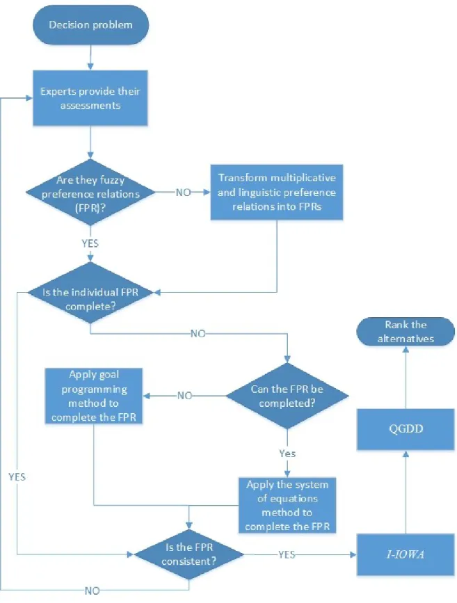
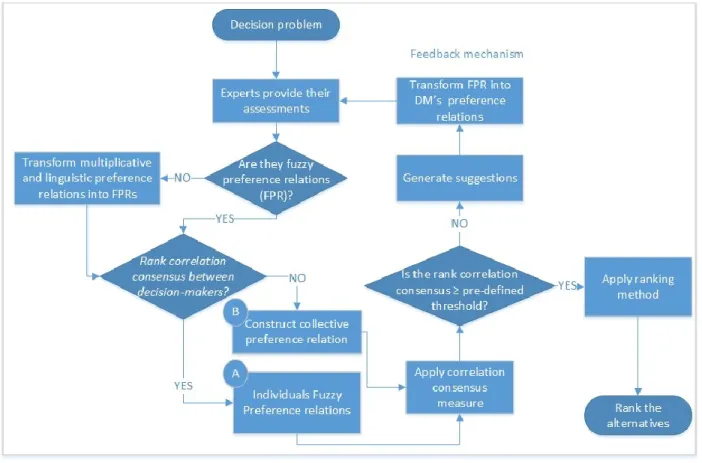
Figure 2.1: Solving incomplete preference relation flowchart ... 39

Figure 3.1: Rank correlation consensus types and relations ... 72

(11)

List of Tables

Table 2.1: Some approaches to solve incomplete preference relations ... 24

Table 2.2: Comparison of the three methods in example 2.3 ... 51

Table 2.3: Comparison of two methods in example 2.4 ... 51

Table 3.1: A brief literature of some consensus measures ... 61

Table 3.2: Rank similarity degrees between decision-makers ... 79

Table 3.3: Rank correlation consensus between DMs ... 80

Table 3.4: Rank similarity degrees between DM 3 and other DMs ... 81

Table 3.5: The new rank correlation consensus ... 83

Table 3.6: Rank correlation consensus between individuals and the collective ... 85

Table 3.7: Proposed method vs. some available methods ... 87

Table 4.1: The causes’ literature of rank reversal ... 95

(12)

List of Acronyms

AHP Analytic Hierarchy Process

BK Borda-Kendall

DC Consistency degree

DEAHP Data Envelopment analysis - Analytic hierarchy process

DM Decision-maker

ELECTRE ELimination and Choice Expressing Reality

GP Goal Programming

I-IOWA Importance induced ordered weighted averaging IOWA Induced ordered weighted averaging

MADM Multi-attributes decision-making MCDM Multi-criteria decision-making

PROMETHEE Preference Ranking Organization Method for Enrichment Evaluations QGDD Quantifier guided dominance degree

rcc Rank correlation consensus

rccd Rank correlation consensus degree rsd Rank similarity degree

RV ranked vector of preference degrees

TOPSIS Technique for Order of Preference by Similarity to Ideal Solution V Vector of preference degrees

WPM Weighted Product Model

(13)

Chapter 1:

Introduction and Background

Decision-making can be done individually or by a group of decision-makers, also known as group decision-making. The group decision is a choice between at least two alternatives made by group members or by group’s leader by consulting the members (Bedau & Chechile, 1984). Individual decision-making is difficult but group decision-making is even harder and complex due to involvement of multiple different preferences making the consensus difficult to reach. Furthermore, individual decisions in small organizations are usually done at lower managerial levels; however, in large organizations group decisions are commonly made at higher managerial levels (Lu et al., 2007).

Three preference representation formats are commonly used in group decision-making: preference orderings (where each individual ranks alternatives from best to worst), utility values (where an individual assigns utility values for alternatives such that the higher the value, the better is the alternative) and preference relations (Herrera-Viedma et al., 2014). Preference relations are based on pairwise comparisons where each pair of alternatives are compared at a time by an expert. Millet (1997) compared five different types of preference elicitation methods and concluded that preferences based on pairwise comparison are more accurate than the others. In group decision-making, some of the decision-makers may not be able to provide complete information about their preferences on the alternatives. That could be related to either the decision-maker not having

(14)

enough knowledge about part of the problem or not being able to discriminate between some of alternatives (Herrera-Viedma et al., 2007b). Thus, the decision-maker gives incomplete preferences where some values are missing.

In group decision-making, two processes are employed: consensus and then selection. The selection process could be applied without adopting consensus through applying the preference relations provided by the decision-makers (Roubens, 1997). This could, however, lead to a solution that might not be accepted by some of the decision-makers, since it does not reflect their preferences (Saint & Lawson, 1994; Butler & Rothstein, 2007). Therefore, they might reject the solution. Thus, consensus is important before applying selection (Kacprzyk et al., 1992). For the selection process, some methods are known to exhibit rank reversal. Rank reversal occurs when a new alternative is added to (or removed from) a set of alternatives, which causes a change in the ranking order of the alternatives (Barzilai & Golany, 1994).

According to Lu et al. (2007), numerous types of decision-making methods can be used in group decision-making problems. Generally, each of these methods follows a rule. Among these rules are:

1. Authority rule: the leader of the group has the authority to make the final decision after holding an open discussion with the members of the group about the decision problem.

a. Advantage(s): the method attains the final decision fast.

b. Disadvantage(s): the method does not takes advantage of the strengths of the experts in the group.

(15)

a. Advantage(s): clear voting rule (democratic participation) and generating fast final decision.

b. Disadvantage(s): the decision may not be well executed because of inadequate discussions among the group.

3. Negative minority rule: the method is based on eliminating the most unpopular alternative one at a time through a vote until only one alternative remains.

a. Advantage(s): good for situations with few experts (voters) and lots of ideas. b. Disadvantage(s): slow method and might lead to discomfort among

decision-makers who are in favor of some eliminated alternatives.

4. Ranking rule: it is based on ranking of the alternatives by the experts. Such a method assigns a number for every alternative by all experts individually. Then the score of each alternative is aggregated. The alternative that has the highest score is selected.

a. Advantage(s): includes voting procedure.

b. Disadvantage(s): might result in a decision not supported by the group.

5. Consensus rule: consensus means full agreement by the group on the decision. The rule is based on reaching decision through discussions and negotiations until all the experts in the group understand and agree with what will be done.

a. Advantage(s): the decision is supported by the group.

b. Disadvantage(s): might be hard to reach consensus and is time consuming.

However, since it is hard and inconvenient to reach full and unanimous agreement among all the experts in the group, besides, a full agreement is not always necessary in practice. A soft consensus

(16)

has been developed, which does not require a full agreement among the experts, relies mainly on consensus measure (Cabrerizo et al., 2010; Herrera-Viedma et al., 2014; Chiclana et al., 2013).

Based on these rules several methods have been developed to improve the processes of group decision-making. The most popular two are Delphi method and multi-voting technique (Lu et al., 2007). Delphi method was developed by Gordon and Helmer in 1953. The method is based on reaching consensus on an opinion without a need from the experts to set together. It could be through survey, questionnaires etc. Several applications of Delphi method have shown its effectiveness in dealing with complex decision problems. Multi-voting technique is used to attain group consensus fast by letting each expert rank the alternatives and collation of the expert’s ranks into the group consensus.

1.1.

A Brief Review

1.1.1. Preference relation preliminary knowledge

Definition 1.1 (Urena et al., 2015): A preference relation 𝑅 is a binary relation defined on the set

𝑋 and is characterized by a function 𝜇𝑝: 𝑋 × 𝑋 → 𝐷, where 𝐷 is the domain of representation of preference degrees provided by the decision-maker.

Definition 1.2 (Urena et al., 2015): An additive preference relation 𝑃 on a finite set of alternatives

𝑋 is characterised by a membership function 𝜇_𝑝: 𝑋 × 𝑋 → [0,1], 𝜇_𝑝(𝑥_𝑖, 𝑥_𝑗) = 𝑝_𝑖𝑗 such that 𝑝_𝑖𝑗 + 𝑝𝑗𝑖 = 1 ∀𝑖, 𝑗 ∈ {1, … , 𝑛}. Furthermore:

(17)

𝑝𝑖𝑗 > 0.5 indicates that the expert prefers alternative 𝑥𝑖 to alternative 𝑥𝑗, with 𝑝𝑖𝑗 = 1 being the maximum degree of preference for 𝑥_𝑖 over 𝑥_𝑗;

𝑝𝑖𝑗 = 0.5 represents indifference between 𝑥𝑖 and 𝑥𝑗; therefore, 𝑝𝑖𝑖 = 0.5.

Let 𝐸 = {𝑒1, 𝑒2, … , 𝑒𝑇} be the set of decision-makers, and 𝑤 = {𝑤1, 𝑤2, … , 𝑤𝑇} be the weight vector of decision-makers, where 𝑤𝑘> 0, 𝑘 = 1,2, … , 𝑇 such that ∑𝑇𝑘=1𝑤𝑘= 1. Then, 𝑃𝑘 =

(𝑝_𝑖𝑗𝑘)_𝑛×𝑛 is the judgment/preference relation of decision-maker 𝑒𝑘∈ 𝐸 on the set of alternatives 𝑋 = {𝑥₁, 𝑥₂, … , 𝑥_𝑛}.

1.1.2. Incomplete preference relations

The individuals in group decision-making come from different background and expertise and each has their motivations or goals. They look at the problem from different angles, yet all have to reach an agreement. Each individual is required to give preferences for a set of pre-determined alternatives. Since each individual has unique experience, he or she may not be able to give a preference degree for some of the alternatives. This could be related to number of reasons. First, they may not have enough knowledge about part of the problem or may not be able to give preferences degrees for some of the alternatives, or decide which alternative is better than the other. In this situation, they provide incomplete information (Herrera-Viedma et al., 2007b) or it can be simply due to time pressure (Xu, 2005a).

Definition 1.3 (Urena et al., 2015): A function 𝑓: 𝑋 → 𝑌 is partial when not every element in the set 𝑋 necessarily maps to an element in the set 𝑌. When every element from the set 𝑋 maps to one element of the set 𝑌 then we have a total function.

(18)

Definition1.4 (Urena et al., 2015): A preference relation 𝑃 on a set of alternatives 𝑋 with a partial membership function is an incomplete preference relation.

A number of papers look at this problem. Xu (2005a) proposed two approaches to find the priority vector of an incomplete fuzzy preference relation based on a system of equations. The first approach uses the system of equations to generate the priority vector of an incomplete fuzzy preference relation. On the other hand, the second approach uses the provided information to estimate the unknown values and then generates the priority vector by the system of equations. Xu (2006) studied five types of incomplete linguistic preference relations, namely, incomplete uncertain linguistic preference relation, incomplete triangular fuzzy linguistic preference relation, incomplete trapezoid fuzzy linguistic preference relation, expected incomplete linguistic preference relation and acceptable expected incomplete linguistic preference relation. Then, based on some transformation functions, he converted them into the expected incomplete linguistic preference relations. He used the expected incomplete linguistic preference relations based on additive consistency to calculate the complete linguistic preference relations. Fedrizzi and Giove (2007) proposed a method based on a linear system to calculate missing values of an incomplete matrix of pairwise comparison. Chiclana et al. (2009) analyzed two methods for estimating missing values in incomplete fuzzy preference relation, one of them being Fedrizzi and Giove’s (2007) method. They ended up with proposing a reconstruction policy for using both methods. Alonso et al. (2008) introduced an iterative procedure to estimate missing information for incomplete fuzzy, multiplicative, interval-valued and linguistic preference relations. Lee (2012) proposed an incomplete fuzzy preference relations method based on additive consistency and order consistency.

(19)

1.1.3. Consensus in group decision-making

Consensus in group decision-making can be interpreted in three ways (Herrera-Viedma et al., 2014). It could mean full agreement or a unanimous decision by the group members or reaching consensus by a moderator who facilitates the process of agreement, or it could mean attaining the consent, where some individuals might not completely agree but are willing to go with the majority opinion of the group. Consensus is the main goal in any group decision-making problem, since obtaining an acceptable solution by the group is important.

Xu (2009) proposed an automatic approach for reaching consensus in multi-attribute group decision-making. His approach was based on numerical settings, where each individual constructs a decision matrix. Then, these matrices are aggregated into one group-decision matrix. The method calculates the similarity measure between each individual matrix and the group decision matrix to determine the degree of consensus. A convergent iterative algorithm is introduced for individual matrices to reach the consensus. Sun and Ma (2015) proposed an approach for consensus using linguistic preference relations. They used consensus measure based on the dominance degree between group preference relation and individuals’ preference relations. Zhang and Dong (2013) proposed an interactive consensus reaching process based on optimization to increase consensus of individuals and minimize the number of adjusted preference values. Guha and Chakraborty (2011) introduced an iterative fuzzy multi-attribute group decision-making technique to reach consensus using fuzzy similarity measures. In addition, their method considers the degrees of confidence of experts’ opinions in the procedure. Herrera-Viedma et al. (2002) proposed a consensus model suitable for four different preference structures. Their model uses two consensus criteria: a consensus measure for measuring the degree of consensus between the experts, and a

(20)

proximity measure to measure the difference between the preferences of individuals and the group preference relation.

1.1.4. Rank reversal

Our literature review on decision-making reveals that a number of methods suffer from the rank reversal phenomenon. These include Analytic Hierarchy Process (AHP) (Barzilai & Golany, 1994; Wang & Luo, 2009), Technique for Order of Preference by Similarity to Ideal Solution (TOPSIS) (Wang et al., 2007; Wang & Luo, 2009), ELimination and Choice Expressing Reality (ELECTRE), Preference Ranking Organisation Method for Enrichment Evaluations (PROMETHEE) (Frini et al., 2012; Mareschal et al., 2008), Data Envelopment analysis - Analytic hierarchy process (DEAHP), Borda-Kendall (BK) (Wang & Luo, 2009 ) and Weighted Sum Method (WSM)( Wang & Luo, 2009), to name a few.

The rank reversal issue has created concerns over the use of the affected methods, especially AHP. Rank reversal could be of two types: partial or total. Partial rank reversal happens to limited alternatives while other alternatives still have the same ordering. Suppose that the current ranking of three alternatives is 𝐴₃ ≻ 𝐴₁ ≻ 𝐴₂, which means that alternative 𝐴₃ is preferred over alternative

𝐴₁ and 𝐴₂ respectively. However, when another non-dominating alternative (𝐴₄) is added, the ranking becomes: 𝐴1 ≻ 𝐴3 ≻ 𝐴4 ≻ 𝐴2. Notice that alternative 𝐴3 now becomes second while alternative 𝐴1 is the first. This is called partial rank reversal. On the other hand, total rank reversal occurs when the whole ordering or ranking is reversed. In this case, the best alternative becomes the worst and the worst becomes the best 𝐴2 ≻ 𝐴4 ≻ 𝐴1 ≻ 𝐴3 (Dymova et al., 2013; Garcia-Cascales & Lamata, 2012).

(21)

Many reasons behind the rank reversal in preference relation have been studied by researchers, especially in AHP. The three main reasons are inconsistency, preference relations aggregation method, and score aggregation method. Dodd et al. (1995) claimed that Saaty’s AHP misses a form of inconsistency within its model, which makes the results doubtful. This claim somehow agrees with Stewart (1992) who stated that rank reversal is a consequence of the way the weights are elicited, ratio scales, and the eigenvector approach. Farkas et al. (2004) blamed inconsistency in pairwise comparison for this issue. Chou (2012) attributes rank reversal in AHP to the aggregation method, due to Saaty’s ratio scale and the inconsistency of judgments.

Other researchers, like Schenkerman (1994), believed that rank reversal in AHP is caused by normalization and its scales seem arbitrary. He claimed that criteria weights are dependent on the alternatives measurements. Thus, any change in the number of alternatives and normalization imposes revision of the criteria weights. Other researchers such as Lai (1995) pointed out that rank reversal happens because of multiplying criteria weights by an unrelated normalized scale of performance ratings. Dyer (1990) claimed that the problem is not just rank reversal, but rather the AHP results’ are arbitrary. This is because the criteria weights may not be right due to the normalization procedure.

1.2.

Scope and Objectives

The scope of our work is limited to additive preference relations in group decision-making. In preference relations settings, decision-makers might not give complete information for their preference degrees on some of the alternatives. In fact, it is unrealistic in group decision-making to acquire all the knowledge about the problem and discriminate between the alternatives,

(22)

especially if the set of alternatives is large (Urena et al., 2015). Thus, it is important and desirable to manage incomplete preference relations by estimating missing information (Urena et al., 2015). Therefore, our first objective in the thesis is to capture decision-maker preferences in numerical settings, particularly additive preference relations, accurately by proposing a method that has the ability to handle incomplete preference relations. Many papers have studied this issue in the general case where at least 𝑛 − 1 non-diagonal preference degrees are given; however, very few papers have studied the ignorance situations. In the ignorance situations, at least one alternative has not been given any preference degree. Thus, our goal is to handle these situations in preference relations.

In group decision-making, reaching a level of agreement between the group members is important even when each member differs from the others. Measuring consensus, aggregation of preferences, and ranking are considered as main issues to be solved in any group decision-making problem (Ben-Arieh & Chen, 2006). Therefore, it is very important to measure consensus degree between individuals and group preference relation to find the similarities. Consensus process in group decision-making involves aggregating individual preferences relations into a collective or group preference relation. Then a similarity measure is used to measure the degree of similarities between the individual matrices and the collective one. If the similarity is greater than or equal to a pre-defined threshold, then the collective preference relation is considered as consensus. Otherwise, the decision-makers with consensus degree below the threshold are asked to re-evaluate their preferences until the consensus degree reaches the acceptable level of similarity. Generally, consensus is an interactive and iterative process where decision-makers revise their preferences until they reach a manageable level of acceptance. Thus, our second objective in this thesis is to

(23)

develop a new consensus measure for group decision-making based on rank correlation, where similarity/distance functions are not the main measures to measure the coherence among decision-makers. A number of papers, such as Perez et al. (2016), Cabrerizo et al. (2015), and Herrera-Viedma et al. (2014) reported that developing a new consensus measure is beneficial to overcome some drawbacks of similarity/distance functions. A study done by Chiclana et al. (2013) compares five different similarity/distance measures of consensus in group decision-making, namely, Manhattan, Euclidean, Cosine, Dice and Jaccard,. They found that different similarity/distance measures could generate significantly different results. Moreover, the chosen measure could affect the speed of convergence for consensus.

The last process in group decision-making is selection. The preference relations are known to have a phenomenon called rank reversal. This phenomenon is considered as an issue by some decision-makers. Thus, they might hesitate to rely on preference relations. For instance, recently Anbaroglu et al. (2014) chose to use Weighted Product Model (WPM) instead of well-known and widely used models such as AHP and WSM just because it does not suffer from any kind of rank reversal issues.Furthermore, they commented on the problem of rank reversal as “a serious limitation” of the multi-criteria decision-making (MCDM) field, which could mislead researchers from understanding the difference between examined alternatives. Therefore, our third objective in this thesis is to solve the rank reversal issue by investigating and addressing its possible causes in additive preference relations. The literature on preference relations, especially multiplicative preference relation, links this phenomenon to inconsistency of the data, the concept of pairwise comparison on which all preference relations are based, preference aggregation method, and score aggregation method. Currently, there is no complete study that investigates these possible reasons

(24)

for rank reversal in preference relations. Leskinen and Kangas (2005) used a regression model to study the inconsistency of pairwise comparisons. They concluded that inconsistency could lead to rank reversal. However, this phenomenon does not occur when there is a single criterion and data is consistent. But, in multiple criteria, even if the data are consistent, the aggregation method or the arithmetic mean can result in rank reversals. Furthermore, to emphasize this issue we pointed out that it violates the contraction consistency condition (𝑐𝑜𝑛𝑑𝑖𝑡𝑖𝑜𝑛 𝛼) [mentioned by Pavlicic (2001), adopted from Amartya Sen] that states:

Contraction consistency condition: If alternative 𝐴 is the best in the set of alternatives 𝑆 such that 𝐴 ∈ 𝑆, then it has to be the best in every subset 𝐸 ⊂ 𝑆 where 𝐴 ∈ 𝐸.

Our aim is to investigate the reasons behind this phenomenon so that they can be prevented or limited when not desired by the group.

1.3.

Thesis Organization

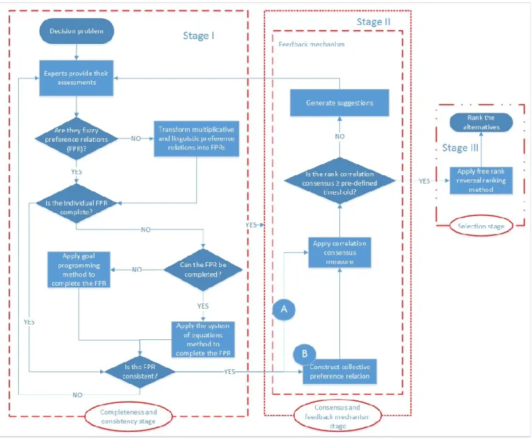
In this thesis, we deal with three associated problems that decision-makers encounter during the process of reaching a final decision in a group decision-making setting. The three problems (challenges) are splits into three stages, where each stage relies on the stage before, as shown in Figure 1.1. In the first stage, we deal with incomplete reciprocal preference relations for missing information in general case and ignorance situations. In the second stage, we deal with the consensus process by proposing a novel consensus measure and feedback mechanism. For the third stage, we study the causes of rank reversal phenomena in preference relations. The rest of

(25)

this thesis is organized based on these contributions, which are presented in Chapters 2, 3 and 4 respectively.

In Chapter 2, we propose two new methods for incomplete reciprocal fuzzy preference relations based on additive consistency. The first method is for the general case where at least 𝑛 − 1 non-diagonal preference degrees are given. This method is based on using a system of equations to estimate the values of missing preference degrees. The second method, based on goal programming, was designed specifically for ignorance situations. It can also be used to estimate values for the general case. In the goal programming model, the objectives are to minimize the errors between the missing preferences degrees and their estimations subject to all the missing preference degrees between 0 and 1.

In Chapter 3, we propose a new consensus measure based on rank correlation to address the consensus among decision-makers. We utilized Spearman’s correlation to measure rank consensus on preference degrees between the decision-makers. Thus, we define ranked preference vector for each decision-maker and develop a new rank similarity degree measure. In addition to measuring rank consensus, we introduce a feedback mechanism to assist the group reach a consensus state.

In Chapter 4, we study the rank reversal in additive preference relations. We investigate the possible causes behind this phenomenon. The study is based on additive consistency. Thereby, we study the link of inconsistency, preference aggregation methods, score aggregation methods and their effect on generating rank reversal. We also propose two new score aggregation methods to handle this phenomenon when it is not desirable by the group. The first score aggregation method is used when a new alternative is added or replaced by the group. In this method, a consistency

(26)

element on the aggregation method is used. The second method is used to prevent rank reversal when an alternative is removed from consideration.

Finally, in Chapter 5 we present the thesis conclusions, contributions, and our perspective for future works.

(27)

(28)

Chapter 2:

Two New Methods for Decision-Making with

Incomplete Reciprocal Fuzzy Preference

Relations Based on Additive Consistency

2.1.

Introduction

Multi-attributes decision-making (MADM) involves making decisions among a set of alternatives with respect to a set of attributes/criteria by a committee of decision-makers. The main idea behind MADM is that the decision-maker (DM) usually faces a problem of selecting an alternative from a number of pre-determined choices, which need to be evaluated based on a number of criteria. Usually, there is no unique or best solution, as the solution is often reached through a compromise: typically, a trade-off between the criteria and decision-makers’ preferences (Hwang & Yoon, 1981). Generally, MADM has issues with regards to the accuracy of decision-maker judgments, the consistency of the judgments, and the method to be used to find the solution (Easley et al., 2000).

In decision-making, there are three commonly used preference representation formats: preference orderings, where each individual ranks alternatives from the best to the worst, utility values, where an individual assigns utility values to alternatives such that the higher the value the better is the alternative, and preference relations (Herrera-Viedma et al., 2014). Preference relations are based

(29)

(1997) compared five different types of preference elicitation methods and concluded that preferences based on pairwise comparison are more accurate than the others.

Fuzzy preference relations are commonly used in decision-making for evaluating a set of alternatives with respect to a set of attributes. However, in some situations, decision-makers may not be able to provide complete information about their preferences on the alternatives. That could be due to the decision-maker not having enough knowledge about part of the problem or being unable to discriminate between some of the alternatives (Herrera-Viedma etal., 2007b) or it might be because of time pressure (Xu, 2005a). In fact, it is unrealistic for all decision-makers to acquire all the levels of knowledge of the whole problem and be able to discriminate between all the alternatives, especially if the set of alternatives is large (Urena et al., 2015). Thus, some decision-makers might not be able to provide information for some of the alternatives. In this case, it is important and desirable to manage incomplete preference relations by estimating the missing information (Urena et al., 2015). Moreover, in some cases, the decision-maker might not be able to give his/her assessments for at least one of the alternatives with respect to the others. This situation is called an ignorance situation and the alternative is called the ignorance alternative (Chen et al., 2014; Alonsoet al., 2009). Most of the existing methods are not compatible with estimating unknown preference degrees for ignorance situations such as the model proposed by Herrera-Viedma etal. (2007a). Furthermore, according to Meng and Chen (2015), other methods try to assign fixed values for the ignorance alternative such as 0 or 0.5.

The main objectives of this work are to solve the problems associated with incomplete preference relations, namely, additive fuzzy preference relation, multiplicative preference relation, and

(30)

linguistic preference relation, when some information is missing or when an ignorance situation is present by:

(1) Proposing a method that has the ability to handle incomplete preference relations with high consistency rate, and also generate a perfect consistent matrix when at least each alternative is compared once.

(2) Proposing a method that solves the ignorance situation with a high consistency level without modifying or changing the decision-maker’s preferences.

The rest of the chapter is organized as follows: we present a brief preliminary knowledge on preference relations in section 2.2. Then a literature review on additive fuzzy preference relations is given in section 2.3 followed by proposed methodology in section 2.4. In section 2.5, the proposed methods are demonstrated with examples. In section 2.6, we validated the proposed methods. Finally, conclusions are given in section 2.7.

2.2.

Preliminary Knowledge

In this section, we provide brief knowledge on three types of preference relations, namely, additive fuzzy preference relation, multiplicative preference relation and linguistic preference relation.

Definition 2.1 (Urena et al., 2015): A preference relation 𝑅 is a binary relation defined on the set

𝑋 that is characterized by a function 𝜇_𝑝: 𝑋 × 𝑋 → 𝐷, where 𝐷 is the domain of representation of preference degrees provided by the decision-maker.

(31)

2.2.1. Fuzzy additive preference relation

Definition 2.2 (Xu, 2007): A fuzzy additive preference relation 𝑃 on a finite set of alternatives 𝑋

is represented by a matrix 𝑃 = (𝑝𝑖𝑗)_𝑛×𝑛 ⊂ 𝑋 × 𝑋 with:

𝑝_𝑖𝑗 ∈ [0,1], 𝑝_𝑖𝑗+ 𝑝_𝑗𝑖 = 1, 𝑝_𝑖𝑖 = 0.5 ∀𝑖, 𝑗 = 1, … , 𝑛.

when 𝑝𝑖𝑗 > 0.5 indicates that the expert prefers alternative 𝑥𝑖 over alternative 𝑥𝑗; 𝑝𝑖𝑗 < 0.5 indicates that the expert prefers alternative 𝑥𝑗 over alternative 𝑥𝑖; 𝑝𝑖𝑗 = 0.5 indicates that the expert is indifferent between 𝑥_𝑖 and 𝑥_𝑗, thus, 𝑝_𝑖𝑖 = 0.5.

Furthermore, the additive preference relation 𝑃 = (𝑝𝑖𝑗)𝑛×𝑛 is additive consistent if and only if the following additive transitivity is satisfied (Meng & Chen, 2015; Urena et al., 2015; Herrera-Viedma etal., 2007a; Tanino, 1984):

𝑝𝑖𝑗+ 𝑝𝑗𝑘 = 𝑝𝑖𝑘+ 0.5 ∀𝑖𝑗𝑘 = 1,2, … , 𝑛. 2.2.2. Multiplicative preference relation

Definition 2.3 (Saaty, 1980): A multiplicative preference relation 𝐴 on the set 𝑋 = {𝑥₁, 𝑥₂, … , 𝑥_𝑛}

of alternatives is defined as a reciprocal matrix 𝐴 = (𝑎𝑖𝑗)𝑛×𝑛 ⊂ 𝑋 × 𝑋 with the following conditions: 𝐴1 𝐴2 … 𝐴𝑛 𝑃 = (𝑝_𝑖𝑗)_𝑛𝑥𝑛 = 𝐴₁ 𝐴2 ⋮ 𝐴_𝑛 [ 0.5 𝑝₁₂ … 𝑝_1𝑛 𝑝₂₁ 0.5 … 𝑝_2𝑛 ⋮ ⋮ ⋱ ⋮ 𝑝𝑛1 𝑝𝑛2 ⋯ 0.5 ]

(32)

𝑎𝑖𝑗 > 0, 𝑎𝑖𝑗𝑎𝑗𝑖 = 1, 𝑎𝑖𝑖 = 1, ∀𝑖𝑗 = 1, 2, … , 𝑛.

where 𝑎_𝑖𝑗 is interpreted as the ratio of the preference intensity of the alternative 𝑥_𝑖 to 𝑥_𝑗.

There are several numerical scales for the multiplicative preference relation, however, the most popular one is the 1-9 Saaty scale. 𝑎𝑖𝑗 = 1 means that alternatives 𝑥𝑖 and 𝑥𝑗 are indifferent; 𝑎𝑖𝑗 >

1 implies that alternative 𝑥_𝑖 is preferred to 𝑥_𝑗. As the ratio of intensity of (𝑎_𝑖𝑗) increases, the stronger is the preference intensity of 𝑥𝑖 over 𝑥𝑗. Thus, 𝑎𝑖𝑗 = 9 means that alternative 𝑥𝑖 is absolutely preferred to 𝑥_𝑗.

The multiplicative preference relation 𝐴 = (𝑎𝑖𝑗)𝑛×𝑛 is called consistent if the following multiplicative transitivity is satisfied (Saaty, 1980):

𝑎_𝑖𝑗 = 𝑎_𝑖𝑘𝑎_𝑘𝑗, 𝑎_𝑖𝑖 = 1, ∀𝑖, 𝑗 = 1, 2, … , 𝑛.

Chiclana et al. (2001) proposed a transformation function to transfer a multiplicative preference relation, 𝐴 = (𝑎_𝑖𝑗)_𝑛×𝑛, into a fuzzy preference relation, 𝑃 = (𝑝_𝑖𝑗)_𝑛×𝑛, as follows:

𝑝𝑖𝑗 =

1

2(1 + log9𝑎𝑖𝑗) ∀𝑖, 𝑗 = 1, 2, … , 𝑛 (2.1)

Moreover, if 𝐴 = (𝑎_𝑖𝑗)_𝑛×𝑛 is a consistent multiplicative preference relation, then the transformed

(33)

2.2.3. Linguistic preference relation

Definition 2.4 (Xu, 2005b): A linguistic preference relation 𝐿 on the set 𝑋 = {𝑥₁, 𝑥₂, … , 𝑥_𝑛} of alternatives is represented by a linguistic decision matrix 𝐿 = (𝑙_𝑖𝑗)_𝑛×𝑛 ⊂ 𝑋 × 𝑋 with

𝑙_𝑖𝑗 ∈ 𝑆̅, 𝑙_𝑖𝑗⊕ 𝑙_𝑗𝑖 = 𝑠₀, 𝑙_𝑖𝑖 = 𝑠₀, ∀𝑖𝑗 = 1, 2, … , 𝑛.

where 𝑙𝑖𝑗 represents the preference degree of the alternative 𝑥𝑖 over 𝑥𝑗. When 𝑙𝑖𝑗 = 𝑠0, means that the decision-maker is indifferent between alternative 𝑥_𝑖 and 𝑥_𝑗; 𝑙_𝑖𝑗 > 𝑠₀ indicates that 𝑥_𝑖 is preferred over 𝑥_𝑗.

Moreover, 𝐿 = (𝑙_𝑖𝑗)_𝑛×𝑛 is consistent when,

𝑙_𝑖𝑗 = 𝑙_𝑖𝑘 ⊕ 𝑙_𝑘𝑗 ∀𝑖, 𝑗, 𝑘 = 1, 2, … , 𝑛.

Let 𝑆 = {𝑠_𝛼|𝛼 = −𝑡, … , −1, 0, 1, … , 𝑡} be a linguistic label set with odd cardinality. Then 𝑠_𝛼

represents a possible value for a linguistic label. In addition, 𝑡 is a positive integer number and

𝑠−𝑡and 𝑠𝑡 are the lower and upper limits of linguistic labels, respectively, while 𝑠0 represents an assessment of “indifference.”

The linguistic label set has following characteristics (Xu, 2004, 2005b):

1. The set is ordered: 𝑠_𝛼> 𝑠_𝛽 if and only if 𝛼 > 𝛽

(34)

In addition, Xu (2004, 2005b) extended the discrete linguistic label set to a continuous set 𝑆̅ = {𝑠𝛼|𝛼 ∈ [−𝑞, 𝑞]} to preserve all the information. In this extension 𝑞 is a large positive integer such that (𝑞 > 𝑡). In general, if 𝑠𝛼∈ 𝑆 then this represents the original linguistic label, otherwise, 𝑠𝛼 is only the virtual linguistic label which appears only in operations.

Let 𝑠𝛼,𝑠𝛽∈ 𝑆̅ and 𝜇, 𝜇1, 𝜇2 ∈ [0, 1]. Some operational laws introduced by Xu (2004, 2005b) are as follows: 1. 𝑠𝛼⊕ 𝑠𝛽 = 𝑠𝛼+𝛽; 2. 𝑠𝛼⊕ 𝑠𝛽 = 𝑠𝛽⊕ 𝑠𝛼; 3. 𝜇𝑠_𝛼 = 𝑠_𝜇𝛼; 4. (𝜇1+ 𝜇2)𝑠𝛼= 𝜇1𝑠𝛼⊕ 𝜇2𝑠𝛼; 5. 𝜇(𝑠_𝛼⊕ 𝑠_𝛽) = 𝜇𝑠_𝛼⊕ 𝜇𝑠_𝛽;

In addition, for any 𝑠∈ 𝑆̅ , 𝐼(𝑠) represents the lower index of , e.g. if 𝑠 = 𝑠_𝛼→ 𝐼(𝑠) = 𝛼 and it is called the gradation of 𝑠 in 𝑆̅. Likewise, we could get the inverse of 𝐼(𝑠): 𝐼−1_{(𝛼) = 𝑠}

𝛼.

An example of the linguistic label set is when 𝑡 = 3, then 𝑆 ={𝑠₋₃= very low, 𝑠₋₂= low, 𝑠₋₁= slightly low, 𝑠₀=medium, 𝑠₁= slightly high, 𝑠₂= high, 𝑠₃= very high}.

Sometimes, depending on the decision problem, experts provide their assessments on the linguistic preference relation using different granularity (multi-granularity). Thus, these granularities need to be unified. Dong et al. (2009) provided following transformation function for unifying multi-granularity into a common multi-granularity (𝑇):

(35)

𝑙_𝑖𝑗 = 𝑇 − 1

𝑇′_{− 1}𝑙𝑖𝑗′ (2.2) where 𝑇 is the intended granularity (normal granularity) and 𝑇′_{is the granularity of}_𝐿′_(𝑙

𝑖𝑗 ′ ₎

𝑛×𝑛.

Dong et al. (2009) and Xu (1999) propose a transformation function to transfer linguistic preference degree (𝑙𝑖𝑗) into fuzzy preference degree based on linear scale function, as follows:

𝑝𝑖𝑗 = 0.5 +

𝐼(𝑙𝑖𝑗)

𝑇 − 1= 0.5 + 𝐼(𝑙𝑖𝑗)

2𝑡 (2.3)

where 𝑇 is the granularity of 𝑆.

2.3.

Literature Review

Preference relations can be categorized into: numeric and linguistic preferences (Urena et al., 2015). The numeric preference relations are of five types: crisp preference relation, additive preference relation, multiplicative preference relation, interval-valued preference relation, and intuitionistic preference relation. On the other hand, there are two main methodologies for linguistic preference relation: linguistic preference relation based on cardinal representation and linguistic preference relation based on ordinal representation.

Many papers have been published about incomplete preference relation in decision-making. Xu (2005a) proposed two approaches to find the priority vector of an incomplete fuzzy preference relation based on a system of equations. The first approach uses the system of equations to generate the priority vector of an incomplete fuzzy preference relation. On the other hand, the second approach uses the provided information to estimate the unknown values and then generates the

(36)

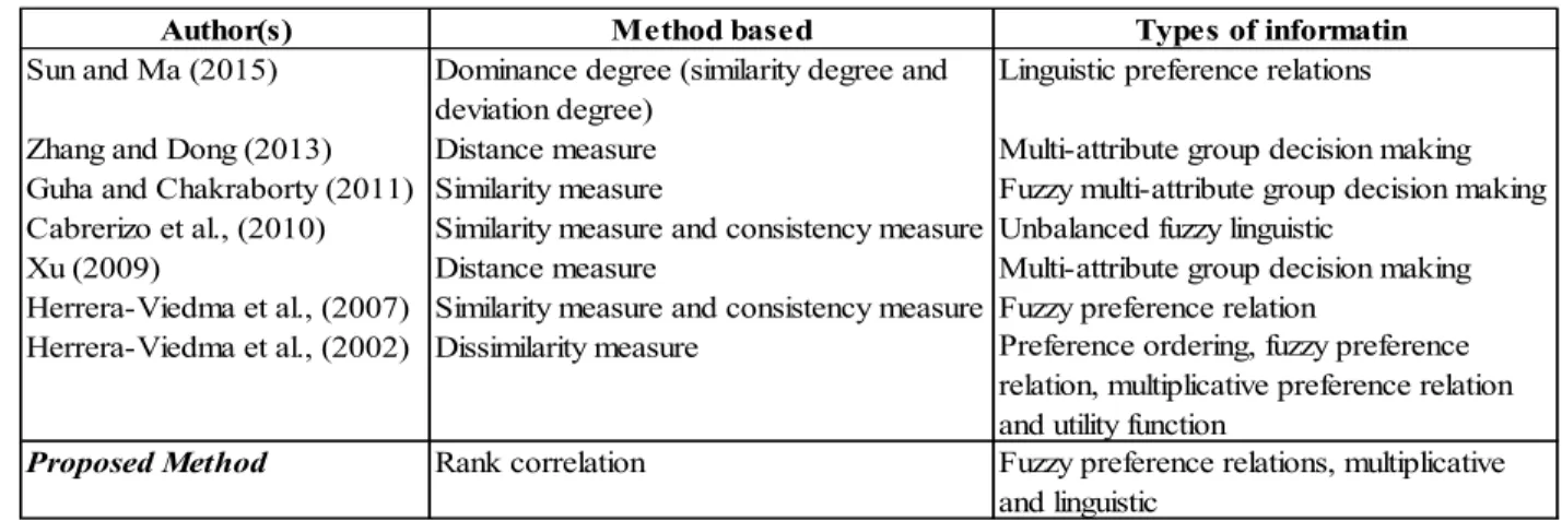
priority vector by the system of equations. Xu (2006) studied five types of incomplete linguistic preference relations, namely, incomplete uncertain linguistic preference relation, incomplete triangular fuzzy linguistic preference relation, incomplete trapezoid fuzzy linguistic preference relation, expected incomplete linguistic preference relation and acceptable expected incomplete linguistic preference relation. Then, based on some transformation functions, he converted them into the expected incomplete linguistic preference relations. He used the expected incomplete linguistic preference relations based on additive consistency to calculate the complete linguistic preference relations. Fedrizzi and Giove (2007) proposed a method based on a linear system to calculate missing values of an incomplete matrix of pairwise comparison. Chiclana et al. (2009) analyzed two methods for estimating missing values in incomplete fuzzy preference relation, one of them being Fedrizzi and Giove’s (2007) method. They ended up with proposing a reconstruction policy for using both methods. Alonso et al. (2008) introduced an iterative procedure to estimate missing information for incomplete fuzzy, multiplicative, interval-valued and linguistic preference relations. Lee (2012) proposed an incomplete fuzzy preference relations method based on additive consistency and order consistency. Table 2.1 summarizes these approaches.

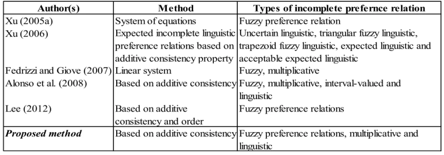
Table 2.1: Some approaches to solve incomplete preference relations

Author(s) Method Types of incomplete prefernce relation

Xu (2005a) System of equations Fuzzy preference relation

Fedrizzi and Giove (2007) Linear system Fuzzy, multiplicative Based on additive consistency

Alonso et al. (2008)

Uncertain linguistic, triangular fuzzy linguistic, trapezoid fuzzy linguistic, expected linguistic and acceptable expected linguistic

Expected incomplete linguistic preference relations based on additive consistency property Xu (2006)

Fuzzy, multiplicative, interval-valued and linguistic

Fuzzy preference relations, multiplicative and linguistic

Based on additive consistency

Proposed method

Fuzzy preference relations Based on additive

consistency and order Lee (2012)

(37)

2.3.1. Incomplete preference relations

Definition 2.5 (Urena et al., 2015): A function 𝑓: 𝐴 → 𝑌 is partial when not every element in the set 𝐴 necessarily maps to an element in the set 𝑌. When every element from the set 𝐴 maps to one element of the set 𝑌, we have a total function.

Definition2.6 (Urena et al., 2015): A preference relation 𝑃 on a set of alternatives 𝐴 with a partial membership function is an incomplete preference relation.

The individuals in group decision-making come from different backgrounds or expertise and each has their motivations or goals in the problem, which might differ from the other members (Urena et al., 2015). Despite that, each individual might look at the problem from a different angle; they all have to interact to reach an agreement. Each individual is asked to give preferences on the set of pre-determined alternatives. However, since each individual has their own experience, they might not be fully aware of the problem and might not give their preferences degree for some of the alternatives. This could be related to number of reasons. They might not have enough knowledge about part of the problem, or they cannot discriminate between the alternatives. Then they do not give their preferences on those alternatives and provide incomplete information (Herrera-Viedma et al., 2007b) or it might be because of time pressure (Xu, 2005a).

In general, incomplete preference relation can be completed based on additive consistency if at least a set of 𝑛 − 1 nonleading diagonal preference values are known and each one of the alternatives are compared directly or indirectly at least once (Xu etal., 2013; Alonsoetal., 2009; Herrera-Viedma etal., 2007a).

(38)

2.3.2. Research gaps

Despite the existing large number of publications on the incomplete preference relation problem, few of them discuss ignorance situations such as Alonso et al. (2009), Chenetal. (2014) and Meng and Chen (2015). Alonso et al. (2009) proposed five strategies for solving the ignorance situation. Two of these strategies are for individual, where the estimation of the missing information depends on the expert without relying on information from other members of the group. The other two are for social, where missing information of the ignorance alternative can be estimated from other members of the group. The last strategy is a hybrid of both individual and social strategies. Chen etal. (2014) solves the drawbacks of Lee’s (2012) method. At the first stage, it assumes that the ignorance alternative is indifferent with respect to the other alternatives. Thus, its preference degrees are equal to 0.5. Then, based on this assumption, the method modifies the consistency, both the additive and the order consistency, of the matrix until it gets to the perfect consistency. Meng and Chen (2015) propose a goal programming method to find the priority vector for incomplete fuzzy preference relation based on additive consistency.

Chen et al. (2014) report that Alonso et al.’s (2009) method violates the property of additive consistency; thus they claim their method is more appropriate, as it satisfies the additive consistency and the order consistency. However, Chen et al.’s (2014) method does not preserve decision-maker preference degrees, at least for the ignorance situation. Nevertheless, all these methods are suitable for certain situations.

Moreover, most of the publications are based on comparing the alternatives directly without explicitly considering the attributes. Incorporating the attributes will make the alternatives

(39)

evaluation process more accurate with deeper understanding of the differences between the alternatives. Although this could increase the number of preference relations, it will increase the confidence of the decision-maker about their assessments on the alternatives and thus the final solution.

2.4.

Proposed Methodology

Transitivity is considered as the main part in defining consistency in decision-making. However, some might argue about its representation to real life individual behavior. One might argue that real life choices could be done in intransitive manner such that an individual might prefer apple over banana and banana over orange but orange over apple. This could be true if the decision was made based on comparing the alternatives directly. However, if a set of certain criteria or attributes has been defined first to draw a judgement on the alternatives, then intransitivity in preference relation under one attribute does not exist. For instance, if we set taste for comparing apple, banana and orange as an attribute, then if the individual prefers the taste of apple over the taste of banana and the taste of banana over the taste of orange, then certainly he or she prefers the taste of apple over the taste of orange. In MADM, the tradeoff between criteria makes maintaining the transitivity among the alternatives hard. However, transitivity within a criterion is a straightforward acquired property.

Therefore, the best adoption to additive consistency is to apply it in MADM concept. The general steps of the decision-making process in MADM as described by Howard (1991), Pohekar and Ramachabdran (2003), and Wang et al. (2009) are:

(40)

2. Generating or choosing the criteria; 3. Identifying the alternatives;

4. Unifying criteria units through normalization; 5. Generating criteria weights;

6. Choosing and applying one of MADM methods; and 7. Selecting the best alternative.

Since we are dealing with preference relations, step 4 is not necessary.

2.4.1. System of equations method

Any incomplete additive preference relation with at least (𝑛 − 1) non-leading diagonal preference degrees can be completed by additive consistency. Additive consistency formulation, which is based on transitivity among preferences degrees, for known 𝑝𝑖𝑗 and 𝑝𝑗𝑘and unknown 𝑝𝑖𝑘is given by:

𝐹1_{: 𝑝}

𝑖𝑘 = 𝑝𝑖𝑗+ 𝑝𝑗𝑘− 0.5 (𝑖, 𝑗) 𝑎𝑛𝑑 (𝑗, 𝑘) 𝑎𝑟𝑒 𝑘𝑛𝑜𝑤𝑛 (2.4)

From this formulation, two other formulations can be generated based on the characteristics of reciprocal rule, (𝑝_𝑖𝑗+ 𝑝_𝑗𝑖 = 1), as follows:

𝐹2_{: 𝑝}

𝑖𝑘 = 𝑝𝑗𝑘− 𝑝𝑗𝑖+ 0.5 (𝑗, 𝑖) 𝑎𝑛𝑑 (𝑗, 𝑘) 𝑎𝑟𝑒 𝑘𝑛𝑜𝑤𝑛, using 𝑝𝑖𝑗 = 1 − 𝑝𝑗𝑖 (2.5)

𝐹3_{: 𝑝}

(41)

Proposition 2.1: Given at least (𝑛 − 1) non-leading diagonal preference degrees, the additive preference relation can be completed for unknown preference degree 𝑝𝑖𝑘 by:

𝑝_𝑖𝑘 = _3(𝑛−2)1 ∑𝑛_𝑗=1 (2𝑝_𝑖𝑗 + 2𝑝_𝑗𝑘− 𝑝_𝑗𝑖 − 𝑝_𝑘𝑗+ 0.5)

𝑖≠𝑗≠𝑘

. (2.7)

Proof: By taking the average of equations (2.4), (2.5) and (2.6) for unknown 𝑝𝑖𝑘 for 𝑛 alternatives, the following equation is generated:

𝑝𝑖𝑘 = 1 3𝑛[∑(𝑝𝑖𝑗 + 𝑝𝑗𝑘− 0.5) 𝑛 𝑗=1 + (𝑝𝑗𝑘− 𝑝𝑗𝑖 + 0.5) + (𝑝𝑖𝑗 − 𝑝𝑘𝑗+ 0.5)] ⟹ 𝑝_𝑖𝑘 = 1 3𝑛∑(2𝑝𝑖𝑗 + 2𝑝𝑗𝑘− 𝑝𝑗𝑖− 𝑝𝑘𝑗+ 0.5) 𝑛 𝑗=1 ⟹ 𝑝_𝑖𝑘 = 1 3𝑛 ∑ (2𝑝𝑖𝑗+ 2𝑝𝑗𝑘− 𝑝𝑗𝑖− 𝑝𝑘𝑗+ 0.5) 𝑛 𝑗=1 𝑖≠𝑗≠𝑘 + 1 3𝑛(𝑝𝑖𝑖+ 𝑝𝑘𝑘 + 4𝑝𝑖𝑘− 2𝑝𝑘𝑖+ 1) ⟹ 𝑝_𝑖𝑘 = 1 3𝑛 ∑ (2𝑝𝑖𝑗+ 2𝑝𝑗𝑘− 𝑝𝑗𝑖− 𝑝𝑘𝑗+ 0.5) 𝑛 𝑗=1 𝑖≠𝑗≠𝑘 + 1 3𝑛(0.5 + 0.5 + 4𝑝𝑖𝑘 − 2(1 − 𝑝𝑖𝑘) + 1) ⟹ 𝑝𝑖𝑘 = 1 3𝑛 ∑ (2𝑝𝑖𝑗+ 2𝑝𝑗𝑘− 𝑝𝑗𝑖− 𝑝𝑘𝑗+ 0.5) 𝑛 𝑗=1 𝑖≠𝑗≠𝑘 + 1 3𝑛(6𝑝𝑖𝑘)

(42)

⟹ (3𝑛)𝑝𝑖𝑘 = ∑ (2𝑝𝑖𝑗+ 2𝑝𝑗𝑘− 𝑝𝑗𝑖 − 𝑝𝑘𝑗+ 0.5) 𝑛 𝑗=1 𝑖≠𝑗≠𝑘 + (6𝑝𝑖𝑘) ⟹ 3(𝑛 − 2)𝑝_𝑖𝑘 = ∑ (2𝑝_𝑖𝑗 + 2𝑝_𝑗𝑘− 𝑝_𝑗𝑖− 𝑝_𝑘𝑗+ 0.5) 𝑛 𝑗=1 𝑖≠𝑗≠𝑘 ⟹ 𝑝_𝑖𝑘 = 1 3(𝑛 − 2) ∑ (2𝑝𝑖𝑗 + 2𝑝𝑗𝑘− 𝑝𝑗𝑖 − 𝑝𝑘𝑗+ 0.5) 𝑛 𝑗=1 𝑖≠𝑗≠𝑘 ∎

The reciprocal rule implies that the matrix could be separated into two portions; upper triangular matrix and lower triangular matrix. Completing any portion will fulfill the other one. Thus, we will focus on completing the upper triangular matrix by using (2.7).

Proposition 2.2: To complete the upper triangular matrix for an incomplete reciprocal additive preference relation with at least (𝑛 − 1) non-leading diagonal preference degrees, the following system of equations is applied:

𝑝𝑖𝑘=_𝑛−21 [∑𝑛𝑗=1 (𝑝𝑖𝑗+ 𝑝𝑗𝑘− 0.5) 𝑖<𝑗<𝑘 + ∑𝑛𝑗=1 (𝑝𝑗𝑘− 𝑝𝑗𝑖+ 0.5) 𝑖>𝑗<𝑘 + ∑𝑛𝑗=1 (𝑝𝑖𝑗− 𝑝𝑘𝑗+ 0.5) 𝑖<𝑗>𝑘 ] ∀ 𝑖 < 𝑘. (2.8)

𝐴

₁

𝐴

₂

𝐴

₃

… 𝐴

_𝑛

𝑃 = (𝑝

_𝑖𝑗

)

_𝑛×𝑛

=

𝐴

₁

𝐴

₂

𝐴

₃

⋮

𝐴

_𝑛

[

0.5

𝑝

₁₂

𝑝

₁₃

… 𝑝

_1𝑛

1 − 𝑝

₁₂

0.5

𝑝

₂₃

… 𝑝

_2𝑛

1 − 𝑝

₁₃

1 − 𝑝

₂₃

0.5

… 𝑝

_3𝑛

⋮

⋱

⋮

1 − 𝑝

_1𝑛

1 − 𝑝

_2𝑛

1 − 𝑝

_3𝑛

⋯ 0.5]

(43)

Proof: 𝑗 could fall in three positions between 𝑖 and 𝑘: 𝑖 < 𝑗 < 𝑘, 𝑖 > 𝑗 < 𝑘 and 𝑖 < 𝑗 > 𝑘. Solve

(2.7) for 𝑝𝑖𝑘 such that 𝑖 < 𝑗 < 𝑘:

𝑝_𝑖𝑘 = 1 3(𝑛 − 2) ∑ (2𝑝𝑖𝑗 + 2𝑝𝑗𝑘− (1 − 𝑝𝑖𝑗) − (1 − 𝑝𝑗𝑘) + 0.5) 𝑛 𝑗=1 𝑖<𝑗<𝑘 ⟹ 1 3(𝑛 − 2) ∑ (3𝑝𝑖𝑗 + 3𝑝𝑗𝑘− 1.5) 𝑛 𝑗=1 𝑖<𝑗<𝑘 ⟹ 1 3(𝑛 − 2) ∑ 3(𝑝𝑖𝑗 + 𝑝𝑗𝑘− 0.5) 𝑛 𝑗=1 𝑖<𝑗<𝑘 ⟹ 𝑝_𝑖𝑘 = _(𝑛−2)1 ∑𝑛_𝑗=1 (𝑝_𝑖𝑗+ 𝑝_𝑗𝑘− 0.5) 𝑖<𝑗<𝑘 ∀ 𝑖 < 𝑗 < 𝑘 (2.8.1)

Solve (2.7) for 𝑝𝑖𝑘 such that𝑖 > 𝑗 < 𝑘:

𝑝𝑖𝑘 = 1 3(𝑛 − 2) ∑ (2(1 − 𝑝𝑗𝑖) + 2𝑝𝑗𝑘− 𝑝𝑗𝑖 − (1 − 𝑝𝑗𝑘) + 0.5) 𝑛 𝑗=1 𝑖>𝑗<𝑘 ⟹ 1 3(𝑛 − 2) ∑ (3𝑝𝑗𝑘− 3𝑝𝑗𝑖 + 1.5) 𝑛 𝑗=1 𝑖>𝑗<𝑘 ⟹ 1 3(𝑛 − 2) ∑ 3(𝑝𝑗𝑘− 𝑝𝑗𝑖 + 0.5) 𝑛 𝑗=1 𝑖>𝑗<𝑘

(44)

⟹ 𝑝_𝑖𝑘 = _(𝑛−2)1 ∑𝑛_𝑗=1 (𝑝_𝑗𝑘− 𝑝_𝑗𝑖 + 0.5)

𝑖>𝑗<𝑘

∀ 𝑖 > 𝑗 < 𝑘 (2.8.2)

Solve (2.7) for 𝑝𝑖𝑘 such that 𝑖 < 𝑗 > 𝑘:

𝑝𝑖𝑘 = 1 3(𝑛 − 2) ∑ (2𝑝𝑖𝑗 + 2(1 − 𝑝𝑘𝑗) − (1 − 𝑝𝑖𝑗) − 𝑝𝑘𝑗+ 0.5) 𝑛 𝑗=1 𝑖<𝑗>𝑘 ⟹ 1 3(𝑛 − 2) ∑ (3𝑝𝑖𝑗 − 3𝑝𝑘𝑗+ 1.5) 𝑛 𝑗=1 𝑖<𝑗>𝑘 ⟹ 1 3(𝑛 − 2) ∑ 3(𝑝𝑖𝑗 − 𝑝𝑘𝑗+ 0.5) 𝑛 𝑗=1 𝑖<𝑗>𝑘 ⟹ 𝑝_𝑖𝑘 = 1 (𝑛 − 2) ∑ (𝑝𝑖𝑗− 𝑝𝑘𝑗+ 0.5) 𝑛 𝑗=1 𝑖<𝑗>𝑘 ∀ 𝑖 < 𝑗 > 𝑘 (2.8.3)

Therefore, (2.7) can be rewritten as a system of linear of equations based on (2.8.1), (2.8.2) and

(2.8.3) for all 𝑖 < 𝑘 as follows:

𝑝_𝑖𝑘 = 1 𝑛 − 2 [ ∑ (𝑝𝑖𝑗+ 𝑝𝑗𝑘− 0.5) 𝑛 𝑗=1 𝑖<𝑗<𝑘 + ∑ (𝑝𝑗𝑘− 𝑝𝑗𝑖+ 0.5) 𝑛 𝑗=1 𝑖>𝑗<𝑘 + ∑ (𝑝𝑖𝑗− 𝑝𝑘𝑗+ 0.5) 𝑛 𝑗=1 𝑖<𝑗>𝑘 ] ∀ 𝑖 < 𝑘∎

(45)

Thus, in the case of the decision-maker giving preference degrees only for 𝑛 − 1 values such that each pair of the alternatives are compared only once, (2.8) can be used to estimate the rest of the unknown values with perfect consistency.

Definition 2.7: Let 𝑃 = (𝑝𝑖𝑘)𝑛×𝑛 be a completed preference decision matrix from (2.8) and

𝑃𝑒_(𝑝

𝑖𝑘𝑒)𝑛×𝑛 be an estimated preference decision matrix from (2.7). Then the consistency degree (DC) between 𝑃 and 𝑃𝑒_{is accepted if and only if} _{𝐶𝐷(𝑃, 𝑃}𝑒_{) ≥ 𝛼}_where_{𝐶𝐷(𝑃, 𝑃}𝑒₎_{is the} consistency degree between 𝑃 and 𝑃𝑒_{, and}_𝛼_{is the least accepted consistency that is defined by} the expert(s).

Saaty (1980) suggested that 𝛼 should be greater than or equal to 90%. In other words, the inconsistency degree should be less than or equal to 10%.

Thus, the consistency degree (similarity degree) between provided (or completed) matrix and the estimated one by additive consistency is:

𝐶𝐷(𝑃, 𝑃𝑒_{) = 1 −} 2 𝑛(𝑛 − 1)∑ ∑|𝑝𝑖𝑘 − 𝑝𝑖𝑘𝑒 | 𝑛 𝑘=2 𝑖<𝑘 𝑛−1 𝑖=1 (2.9)

2.4.2. Goal programming model

Based on (2.8), multi-objective programming model is introduced. The model objectives are to find the errors between the missing preferences degrees and their estimations. Thus, the solution to the missing preferences degrees can be obtained by solving the following multi-objective

(46)

programming model, where the objectives are to minimize the errors between the missing preferences degrees and their estimations subject to all missing preferences between 0 and 1.

(𝑀𝑂𝑃) min 𝜀𝑖𝑘 = ∑ ∑ ||𝑝𝑖𝑘 𝑛 𝑘=2 𝑖<𝑘 𝑛−1 𝑖=1 − 1 𝑛 − 2 [ ∑ (𝑝𝑖𝑗+ 𝑝𝑗𝑘− 0.5) 𝑛 𝑗=1 𝑖<𝑗<𝑘 + ∑ (𝑝𝑗𝑘− 𝑝𝑗𝑖+ 0.5) 𝑛 𝑗=1 𝑖>𝑗<𝑘 + ∑ (𝑝𝑖𝑗− 𝑝𝑘𝑗+ 0.5) 𝑛 𝑗=1 𝑖<𝑗>𝑘 ] || 𝑠. 𝑡. 𝑝𝑖𝑘 ∈ [0, 1] 𝑖 = 1, 2, … 𝑛 − 1; 𝑘 = 2, 3, … 𝑛; 𝑖 < 𝑘 𝑝𝑘𝑖 = 1 − 𝑝𝑖𝑘 𝑖 = 1, 2, … 𝑛 − 1; 𝑘 = 2, 3, … 𝑛; 𝑖 < 𝑘

The solution to the above multi-objective programming model is found by solving the following goal programming model.

(𝐺𝑃) min 𝑧 = ∑ ∑(𝑑_𝑖𝑘+ _{+ 𝑑} 𝑖𝑘−) 𝑛 𝑘=2 𝑖<𝑘 𝑛−1 𝑖=1 𝑠. 𝑡. 𝑝_𝑖𝑘− 1 𝑛 − 2 [ ∑ (𝑝_𝑖𝑗 + 𝑝_𝑗𝑘− 0.5) 𝑛 𝑗=1 𝑖<𝑗<𝑘 + ∑ (𝑝_𝑗𝑘− 𝑝_𝑗𝑖+ 0.5) 𝑛 𝑗=1 𝑖>𝑗<𝑘 + ∑ (𝑝_𝑖𝑗− 𝑝_𝑘𝑗+ 0.5) 𝑛 𝑗=1 𝑖<𝑗>𝑘 ] − 𝑑_𝑖𝑘+ + 𝑑_𝑖𝑘− _{= 0 𝑖 = 1, 2, … 𝑛 − 1; 𝑘 = 2, 3, … 𝑛; 𝑖 < 𝑘} 𝑝_𝑖𝑘 ∈ [0, 1] 𝑖 = 1, 2, … 𝑛 − 1; 𝑘 = 2, 3, … 𝑛; 𝑖 < 𝑘

(47)

𝑝_𝑘𝑖 = 1 − 𝑝_𝑖𝑘 𝑖 = 1, 2, … 𝑛 − 1; 𝑘 = 2, 3, … 𝑛; 𝑖 < 𝑘 𝑑_𝑖𝑘+ _{∗ 𝑑} 𝑖𝑘− = 0 𝑖 = 1, 2, … 𝑛 − 1; 𝑘 = 2, 3, … 𝑛; 𝑖 < 𝑘 𝑑_𝑖𝑘+_{, 𝑑} 𝑖𝑘 − _{≥ 0}

where 𝑑_𝑖𝑘+ is the positive deviation from the goal 𝜀𝑖𝑘 and 𝑑𝑖𝑘− is the negative deviation from the goal 𝜀_𝑖𝑘.

The model objectives are to minimize the deviations from the target of the goal subject to the same constraints as the multi-objective model. In addition to the errors between the missing preferences degrees and their estimations, the product of the positive and negative deviations from the goal should be equal to 0 and that all the decision variables are greater than or equal to 0.

2.4.3. Algorithm for group decision-making with incomplete fuzzy preference relations

In any group decision-making problem, there are usually two processes: A) consensus process and B) selection process. Since our focus is on completing the information, we will apply the selection process. The selection process consists of two phases, aggregation phase and exploitation phase as follows:

A. Aggregation phase

This phase constructs a collective preference relation by aggregating the provided preference relations by the decision-makers. The aggregation will be conducted by an importance-induced ordered weighted averaging (I-IOWA) operator.

(48)

Importance induced ordered weighted averaging (I-IOWA) operator

Importance-induced ordered weighted averaging (I-IOWA) is a modified aggregation operator of induced ordered weighted averaging (IOWA) proposed by Chiclana et al. (2007). This operator is based on transferring the original preference values into new values by using the decision-makers’ importance degrees. First, we introduce the definition of (IOWA) as follows:

Definition 2.8 (Chiclana et al., 2007): An IOWA operator of dimension 𝑛 is a function 𝛷_𝑊: (ℝ × ℝ)𝑛 _{→ ℝ}_{, to which a set of weights or weighting vector is associated,}_{𝑊 =}

(𝑤1, 𝑤2, … , 𝑤𝑛 ), such that 𝑤𝑖 ∈ [0, 1] and ∑ 𝑤𝑛𝑖 𝑖 = 1, to aggregate the set of second arguments of a list of n 2-tuples {〈𝑢1, 𝑝1〉, … , 〈𝑢𝑛, 𝑝𝑛〉} according to the following expression:

𝑃𝑐 _{= 𝛷}

𝑊(〈𝑢1, 𝑝1〉, … , 〈𝑢𝑛, 𝑝𝑛〉) = ∑ 𝑤𝑖 𝑛

𝑖=1

∗ 𝑝𝜎(𝑖)

being 𝜎: {1, . . . , 𝑛} → {1, . . . , 𝑛} a permutation such that 𝜇_𝜎(𝑙) > 𝜇_𝜎(𝑙+1) is the 2-tuple with 𝜎(𝑖)

the 𝑖th_{highest value in the set}_{{ 𝜇}

1, 𝜇2, … , 𝜇𝑛}.

The associated weights of the IOWA operator are obtained by

𝑤𝑘= 𝒬 (

𝑆(𝑘)

𝑆(𝑛)) − 𝒬 (

𝑆(𝑘 − 1) 𝑆(𝑛) ), ∀𝑘

where 𝑘 = {1, 2, … , 𝑛}, 𝑆(𝑘) = ∑𝑘𝑙=1𝜇𝜎(𝑙), 𝑆(𝑛) = ∑𝑛𝑙=1𝜇𝑙, and 𝜎 is the permutation such that

𝜎(𝑘) is the 𝑘th_{largest value in the set}_{{ 𝜇}

(49)

The associated weights (𝑤𝑘) are obtained by using a fuzzy majority concept and a fuzzy linguistic quantifier. There are several common fuzzy linguistic quantifiers such as all, most of, and as many as possible.

Definition 2.9 (Chiclana et al., 2007): If a set of experts, 𝐸 = {𝑒1, . . . , 𝑒𝑚}, provide preferences about a set of alternatives, 𝑋 = {𝑥₁, . . . , 𝑥_𝑛}, by means of the fuzzy preference relations,

{𝑃1_{, . . . , 𝑃}𝑚_}_{, and each expert}_𝑒

𝑘 has an importance degree, 𝜇𝐼(𝑒𝑘) ∈ [0, 1], then an I-IOWA operator of dimension 𝑛, 𝛷_𝑊𝐼 _{, is an IOWA operator whose set of order inducing values is the set} of importance degrees.

B. Exploitation phase

By using the information of the collective preference relation, the alternatives are ranked from the best to the worst. The ranking of the alternatives will be obtained by using quantifier guided dominance degree (QGDD). This is used to quantify the dominance that one alternative has over the others, as follows:

𝑄𝐺𝐷𝐷_𝑖 = 𝛷_𝑊(𝑝_𝑖𝑗𝑐_{, ∀𝑗 = 1, … , 𝑛) = ∑} _𝑤 𝑗 𝑛

𝑗=1 ∗ 𝑝𝜎(𝑗)𝑐

Where 𝜎(𝑗) is the 𝑗th_{highest value in the}_(𝑝

𝑖𝑗𝑐, ∀𝑗 = 1, … , 𝑛).

Thus, to solve any preference relation with incomplete information, different types of preference relation, i.e. linguistic or multiplicative preference relations, need to be transformed into a fuzzy additive preference relation. Then the following steps apply