Sprottivas And Implications For Productivity

Retrading, production, and asset market performance

Steven D. Gjerstad, David Porter, Vernon L. Smith1, and Abel Winn

Economic Science Institute, Argyros School of Business and Economics, Chapman University, Orange, CA 92866

Contributed by Vernon Smith, August 31, 2015 (sent for review June 8, 2015; reviewed by Gunduz Caginalp and Charles N. Noussair) Prior studies have shown that traders quickly converge to the

price–quantity equilibrium in markets for goods that are immedi-ately consumed, but they produce speculative price bubbles in re-salable asset markets. We present a stock-flow model of durable assets in which the existing stock of assets is subject to deprecia-tion and producers may produce addideprecia-tional units of the asset. In our laboratory experiments inexperienced consumers who can resell their units disregard the consumption value of the assets and compete vigorously with producers, depressing prices and production. Consumers who have first participated in experi-ments without resale learn to heed their consumption values and, when they are given the option to resell, trade at equilib-rium prices. Reproducibility is therefore the most natural and most effective treatment for suppression of bubbles in asset mar-ket experiments.

durable assets

|

stock-flow markets

|

specialization of trade

|

asset market bubbles

C

ontrary to rational theory the first asset market experiments with complete common information on fundamental value exhibited unexpectedly strong tendencies to yield price bubbles (1). The results, however, were soon extended (2, 3), indepen-dently replicated (4–8), and have quite important consequences for improved understanding of the sources of instability in the economy (9–11).

In contrast with these robust asset market findings, earlier experiments had established that repeated trade across time periods in static supply and demand experiments yielded effi-cient rapid convergence to rational competitive equilibrium outcomes under strictly private decentralized information (12). In the supply and demand experiments, however, trades were for immediate consumption, as with hamburgers and haircuts; as noted in ref. 13, items could not be retraded and individuals knew in advance that they were specialized as buyers or sellers and could not switch roles depending on price as in asset markets. [These features also characterize nondurable goods and services in the US national accounts and represent approximately 75% of private product. Instability in the US national accounts arises from the remaining 25% (11)].

Motivated by the glaring contrast in these two kinds of mar-kets, Dickhaut et al. (13) reformulated the traditional supply and demand environment by explicitly modeling two goods:“cash”as a means of payment and a“commodity” that had a heteroge-neous end-of-period“dividend” consumption yield value. This formulation exactly parallels the asset trading environment, ex-cept that cash and commodity endowments have only a one-period life and dividends are not common. Individual subjects received diverse endowments, but in each of 10 periods a subject was endowed with the same amounts of cash and commodity, thus inducing pure static supply and demand conditions across 10 periods. This reformulated framework allowed the study of convergence in a 2×2 design, (retrade, no retrade)×(low cash, high cash). Convergence was markedly slower in retrade vs. no retrade because traders who could retrade had difficulty learning from market prices their optimal role as buyers or sellers. High cash exacerbated this difficulty relative to low cash, in line with previous findings (14).

Haruvy et al. (ref. 15, p. 7) observe that because durable goods can be retraded they carry an implicit option value for resale at a higher or lower price depending on individual ex-pectations. [Harrison and Kreps (16) also demonstrated this possibility in a theoretical model.] A perishable good has only consumptive utility value, if purchased, whereas a durable good will yield consumptive value if retained, but a resale value if not. Thus, durable goods can involve a speculative motive whereas nondurables cannot. It is this speculative motive that has driven price bubbles in studies of asset markets.

Previous studies have modeled a durable asset whose life extends over the entire horizon of the experiment; in those studies—unlike house or automobile markets, for example— no new units were produced and existing units did not de-preciate during the course of the experiment. [However, Haruvy et al. (15) study a securities market subject to external interventions to repurchase existing shares that reduce the asset stock, or issue new shares that increase the stock.] In this paper we model producers who at private unit cost may elect to sell newly produced units that add to the existing stock; also, we introduce an elementary“replacement demand” for asset units: The existing units “depreciate”with a constant proba-bility, independent of age and price. Hence, there is a net addition (or loss) of asset units in the market depending on whether production is greater than or less than the deprecia-tion rate. We set the stage for experimental studies of asset market trading characterized by dynamic stock-flow trajecto-ries over time with the stock determined endogenously. [Ab-stract general stock-flow models were introduced by Clower (17) for capital asset pricing and Smith (18) for the theory of the firm.] In our new experiments we find that resale inhibits price discovery, which in turn distorts production and retards efficiency. However, whereas resale has generated price bub-bles in asset markets without production, in our asset markets resale suppresses prices well below equilibrium. This is be-cause many consumers fail to specialize as buyers, and instead compete with producers as sellers. When we rerun the resale ex-periments with subjects who are experienced as specialized buyers and sellers in the no-resale treatment prices and production converge to equilibrium and efficiency improves. Reproduc-ibility is therefore the most natural and most effective treatment

Significance

We conduct the first experimental study to our knowledge of production and trade in a stock-flow market for durable assets. When inexperienced consumers are allowed to resell assets they compete with producers and depress prices, disrupting production and causing inefficiency. Consumers with experi-ence specializing as buyers compete less vigorously, which al-lows prices and production to converge to equilibrium. Author contributions: S.D.G., D.P., and V.L.S. designed research; A.W. performed research; S.D.G., D.P., and V.L.S. contributed new reagents/analytic tools; A.W. analyzed data; and S.D.G., D.P., V.L.S., and A.W. wrote the paper.

Reviewers: G.C., University of Pittsburgh; and C.N.N., Tilburg University. The authors declare no conflict of interest.

Freely available online through the PNAS open access option.

1_{To whom correspondence should be addressed. Email: [email protected].}

ECO

NOMIC

for suppression of bubbles in asset market experiments. [Hong et al. (19) develop a theoretical model in which release of locked up shares can suppress a price bubble following an initial public offering.]

Theoretical Model

Our model of a reproducible durable asset has several key ele-ments. First, asset units provide use value to their owners, which we refer to as dividends. Dividends represent the stream of services to an owner occupying his home or the rental stream to a landlord. The asset yields a dividend but also has some persis-tence. Depreciation is a common feature of durable assets, in-cluding residential, commercial, and industrial structures. We assume that an asset unit depreciates with probability μ, in-dependent of its age. (As a result of this idealization units are homogeneous.) If μ> 0 then the dividends received from an asset unit have a finite expected value, which we assume repre-sents its value to a consumer. Individual demand is functionally determined from the unit values to a consumer, and market demand is the aggregation of the individual demands. Theoret-ically, price at any time is determined from the condition that the market demand is equal to the supply, which is the current stock of units available. Suppliers can profitably sell newly produced units if their cost is below the market price. The total produced less the loss from depreciated units is the increment to the stock of asset units in the subsequent period. These elements consti-tute the model, formally described below.

Asset Life.We assume that at times t=1, 2, 3,. . .an asset unit depreciates with probability μ. The probability that a unit de-preciates is independent for each unit. In particular, it does not depend upon the time period a unit was produced.

Dividends.We assume that consumerireceives a dividenddðjÞ_i ðtÞ for thejthunit thati owns in periodt. In our experiments unit j yields a constant dividend in each period that it is owned by consumer i, so we suppress the time variable and denote the dividend bydðjÞi . An asset purchased or held at timetpays a dividend at timetwith certainty, but immediately after the div-idend is paid it depreciates with probability μ. The probability that the asset unit pays a dividend in periodt+1 is 1–μ, so its expected value in the next time period isð1−μÞdðjÞ_i . The proba-bility that the asset unit lasts from periodtuntil at least period t+kisð1−μÞk, so at timetthe expected value of the dividends from the asset unit in periodt+kisð1−μÞkdðjÞ_i . The expected value of the asset unit services from periodtonward is

V_iðjÞðtÞ=X ∞ k=0 ð1−μÞk_dðjÞ i =dðjÞ_i . μ. [1]

Because the value of unitj for consumeridoes not depend on the time when it is purchased, we write V_iðjÞ=dðjÞ_i =μ. We also assume that dðjÞ_i ≥dðj_i+1Þ for all j because a consumer will put the first unit purchased to its most valuable use.

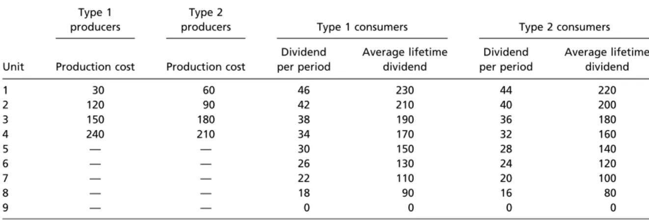
Demand and Asset Stock.If consumers have the per-period divi-dends and average lifetime dividivi-dends shown in Table 1 thenP= D−1_{(Q)=235−2.5 * Q is a linear approximation to the market} inverse demand function. In this case Q=D(P)=94–0.4 * P is a linear approximation to the market demand.

The theoretical market price is determined from the demand and the stock of asset units. Fig. 1 shows an example market demand D(P)=94–0.4 * P and a stock of X(0)=22 asset units. The equilibrium price in this market is determined from X(0)= D(P*) so P* = 180. All of these elements are shown in Fig. 1,Left.

Producers’Costs and Market Supply.In our experimentμ=0.2 so that on average 20% of the asset stock depreciates in time t. With the costs shown in Table 1, the market inverse supply function is approximated by P=S−1(Q)=15 * Q+15, so market supply is approximated by Q=S(P)=P/15–1. With the short-run equilibrium price of P*= 180 producers will add Q*=11 units to the market. Becauseμ=0.2, 4.4 units can be expected to depreciate. Hence, 6.6 units are added to the stock of assets, as shown in Fig. 1,Right.

Steady State.Production and depreciation at timetdetermines the asset stock at time t+ 1. This results in a new short-run equilibrium price, production and depreciation at t + 1, de-termining the asset stock att+2. The process reaches a steady state—if it exists—that is characterized by the conditions XðtÞ=DðPpÞand SðPpÞ=μXðtÞ. That is, the price is set where demand intersects the stock of asset units and at this price production replaces the units that depreciate. Given the pa-rameters in Table 1 and a depreciation rate of 20%, the steady state occurs with an asset stock of 40 units. The resulting price of 135 would elicit 8 units of production, exactly offsetting the 20% depreciation of the 40 units of stock.

Table 1. Induced values and costs for consumers and producers Type 1

producers

Type 2

producers Type 1 consumers Type 2 consumers

Unit Production cost Production cost

Dividend per period Average lifetime dividend Dividend per period Average lifetime dividend 1 30 60 46 230 44 220 2 120 90 42 210 40 200 3 150 180 38 190 36 180 4 240 210 34 170 32 160 5 — — 30 150 28 140 6 — — 26 130 24 120 7 — — 22 110 20 100 8 — — 18 90 16 80 9 — — 0 0 0 0

In our experiments each consumer had a carrying capacity of nine units; each producer could produce up to four units per period. The probability of deterioration after a given period was 0.2, so a unit had an expected lifetime of five periods.

Experiment Design

We tested our durable goods model under two treatment condi-tions, both of which used a double auction to mediate trade. In the baseline treatment (BL) we suppressed the asset units’option risk by requiring units that were purchased in the BL to be held until they depreciated. In the resale treatment (RS) we allowed con-sumers to freely resell their units to one another. Producers were not allowed to purchase units in either treatment; speculation could occur only among consumers. In our RS treatment the resale option risk hindered prices from converging to equilibrium and degraded market efficiency. We then conducted additional sessions under the RS condition using participants with prior experience in the BL. We refer to these sessions as resale with experience (RSX).

Experiment Parameters. The laboratory experiments implement the discrete approximated supply and demand functions shown in Table 1. Our approximations preserve the long-run equilib-rium price, stock, and flow predictions described above. We allocated holding values and production costs among eight consumers and four producers. Induced costs and values were described in terms of experiment currency units (ECUs). (The exchange rate for ECUs to dollars was 75 to 1 for consumers and 50 to 1 for producers.)

All experiment sessions lasted 16 periods, each consisting of a production phase followed by a trading phase. The producers had 30 s to decide how many units to produce, with a maximum of four units each. Producers who did not finalize their pro-duction decision within the time limit produced no units for that period. Producers’inventories carried over, so that if a unit went unsold in the period in which it was produced it could be sold in a subsequent period. Units in inventory did not depreciate. At the outset of the experiment every producer was endowed with starting capital of 520 ECUs, allowing each to produce up to three units. Funds for additional production had to be earned by selling units. The 520 ECUs were reclaimed from a producer’s earnings at the end of the session.

The duration of the trading phase varied by period. For the first five periods subjects had 3 min to execute their trades. As subjects gained experience with the trading process the duration was reduced to 2.5 min for periods 6–10 and reduced again to 2 min thereafter.

We described a unit’s consumption value to the consumers as a dividend that it would pay them at the end of each period until it depreciated (or was sold in the RS and RSX). Every asset unit had probabilityμ=0.2 of deteriorating per period and did not depreciate until after it had earned its dividend for the period. (Units depreciated independently; more or less than 20% of units could depreciate in a period.) Consequently, all units had an expected lifetime of five periods and the expected earnings

from holding a unit was five times its dividend per period. We described these expected earnings to the consumers as a unit’s average lifetime dividend (ALD).

Risk-neutral consumers with no speculative motive should not be willing to pay any more than the ALD for an asset unit. (In the resale treatments, they should not be willing to accept less than the ALD for a unit.) Units that had not depreciated by the end of period 16 continued to pay dividends through a number of periods that continued until all units had depreciated. This en-sured that a unit’s ALD did not diminish in the last few periods of the experiment. During these simulations, production and trade did not occur. The only activity was the payment of dividends and the usual probabilistic decay of asset units.

The consumers received an income of 400 ECUs per period, which they could use to buy units. In our model agents split consumption between the durable asset and a composite com-modity; they do not carry cash holdings across time periods. We implemented this in the experiments by sequestering all divi-dends, unspent income, and cash earned from resale (in the RS and RSX) at the close of the trading phase. The sequestered amount was added to a consumer’s total earnings, which was visible on her computer screen. We subtracted 6,000 ECUs— that is, their cash income for 15 of the 16 trading periods—from their total earnings at the end of the experiment. This ensured that the majority of earnings came from activity in the asset market rather than from passively collecting income.

The producers’cost schedules are presented in the second and third columns of Table 1. The four producers were split evenly into two types. Type 1 producers had a cost advantage on their first and third units, whereas type 2’s had a cost advantage on their second and fourth units. The fifth and seventh columns of Table 1 contain the consumers’value schedules. The eight consumers were also split evenly into two types. Type 1 consumers’dividends were 2 ECUs

Fig. 1. Unit stocks and flows from a sample environment. If we assume that in time period 0 the initial stock is 22 units, the equilibrium price in that period will be P0*=180. This price elicits 11 units of production, and 20% of the initial stock deteriorates. The resulting increment to the stock is 6.6 units, which is shown by the short dashed lines (Right). The process is iterated; in the limit the process reaches a steady state with a stock of 40 units. The price of 135 elicits 8 units of production, which is exactly offset by 20% depreciation of the 40 units of stock.

Table 2. Results of random effects regression models of consumers’share of sales and percent of resales that were surplus-enhancing

Independent variable

Consumers’sales share, coefficient (SE) % Efficient resale, coefficient (SE) Constant 0.840*** (0.030) 0.535*** (0.033) RSX −0.280*** (0.054) 0.113†(0.076) Period −0.021*** (0.002) −0.007* (0.003) RSX×period 0.001 (0.004) 0.005 (0.006) Observations 208 207 Waldχ2 _{180.09 33.97} R2 _{0.5911 0.1434} Significant at†10%, *5%, **1%, or ***0.1%. ECO NOMIC SCIENCES

higher than type 2’s for all units except for unit 9, which was worth 0 to both types. The ninth unit allowed for the possibility of purely speculative purchases in the RS and RSX.

In the first period we endowed half of the consumers (two of each type) with seven units and the other half with six units. This generated an initial asset stock of 52 units, 12 more than the long-run equilibrium. Consequently, the short-run equilibrium prices were predicted to increase as the excess units depreciated. This allows us to test the ability of traders to track the short-run equilibrium and achieve the long-run steady state. Increasing prices in the early rounds also presented the possibility of in-ducing a speculative price bubble in the RS and RSX by en-couraging consumers to expect the prices to continue to rise. Methods. The subjects interacted via computers separated by privacy dividers. They first read through interactive instructions on their screens explaining the rules of the experiment and their user interface. After completing the instructions the subjects participated in a single practice period that did not affect their earnings or unit holdings during the actual experiment.

We conducted nine sessions of both the BL and RS treatments, and four sessions of the RSX. The subject sample consisted of 264 undergraduate and graduate students from Chapman University who were recruited at random from a database of∼2,000. Aside from the RSX no subjects participated in more than one session. In addition to earnings based on their decisions we paid subjects $7 for attending the BL and RS sessions and $15 for attending the RSX. (The higher RSX attendance payment was to encourage partici-pation due to the smaller pool of potential participants.) The av-erage decision-based earnings were $27.81 in the BL, $23.02 in the RS, and $26.35 in the RSX.

Results

We examine differences in resale between the RS and RSX treatments, as well as the performance of all treatments on con-vergence to the equilibrium price and production levels, and effi-ciency. We analyze the data with a set of random effects regression models. For resale the dependent variables are a treatment dummy for the RSX, a time trend variable, and an interaction of the time trend and treatment dummy (Table 2). For prices, production, and efficiency the dependent variables are treatment dummies for the RS and RSX, a time trend variable, and interactions of the time trend with each treatment dummy (Table 3).

The price and production data showed nonlinear convergence, so the regression models for these data use the log of the period for the time trend. Trader performance changed with experience and the estimated time trends are often different across

treatments, so we calculated the model estimates for each treatment in each period and used Wald tests to compare these estimates across treatments and/or to theoretical predictions. We report the results of these tests where appropriate.

Result 1.There was less resale in RSX than RS, and resale in the RSX increased efficiency more frequently. Resale could enhance welfare by reallocating units from consumption values below the market clearing price to values above it. We analyze consumer resale with two metrics: the percent of all trades in a period in which a consumer was the seller (i.e., consumers’sales share) and the percent of resale in a period in which the buying consumer valued the unit more highly than the selling consumer (i.e., efficient resale rate).

Our regression model demonstrates that consumers in the RS failed to optimally specialize as buyers, instead competing as sellers with the producers. The estimated constant indicates that at the start of the RS treatment consumers were the sellers in 84% of all trades (P<0.001). Consumers who were experienced in the BL were more specialized as buyers. The RSX dummy indicates that the consumers’ sales share was 28 percentage points lower at the start of RSX than in the RS (P<0.001). The main time trend estimate is−0.021 (P<0.001), indicating that consumers became more specialized over time in the RS. How-ever, experience had the same effect in the RSX. The time trend interaction term is statistically insignificant (P=0.509).

Resale was more efficient when the consumers were experi-enced. Our regression model estimates that the initial rate of efficient resale in the RS was 53.5%. This is not significantly Table 3. Results of random effects regression models of price deviation from the short-run equilibrium, production deviation from the optimal response, production efficiency, and trade efficiency

Independent variable Price deviation, coefficient (SE) Production, coefficient (SE) Production efficiency, coefficient (SE) Trade efficiency, coefficient (SE) Global efficiency, coefficient (SE) Constant 27.40* (11.09) 9.13*** (0.44) 0.846*** (0.027) 0.787*** (0.048) 0.667*** (0.049) RS −71.99*** (15.68) −3.24*** (0.63) 0.060 (0.038) −0.155* (0.068) −0.091 (0.069) RSX −37.07†(19.99) −2.50** (1.07) 0.116* (0.048) −0.019 (0.086) 0.074 (0.088) Period 0.008*** (0.001) 0.005 (0.004) 0.011** (0.004) RS×period −0.017*** (0.002) −0.012* (0.006) −0.22*** (0.005) RSX×period 0.007** (0.002) −0.003 (0.008) −0.009 (0.007) Log(period) −22.64*** (5.49) −0.88** (0.32) RS×log(period) −8.04 (7.77) −0.57 (0.45) RSX×log(period) 23.21* (9.90) 1.77** (1.23) No. of observations 352 352 330 330 330 Waldχ2 _{80.20 89.12 96.35 47.25 56.22} R2 _{0.5311 0.5544 0.3296 0.2532 0.3470} Significant at†10%, *5%, **1%, or ***0.1%.

Fig. 2. Average deviation of price from the short-run equilibrium by treat-ment.♢, BL;○, RS;□, RSX.

higher than 50%, the rate we would expect if consumers in the RS resold their units at random (Wald test,P=0.357). The estimated coefficient of the RSX dummy is positive and indicates an initial efficient resale rate of 64.8%. This estimate is only marginally significant compared with the RS (P = 0.061), but experienced consumers outperformed random resale. A Wald test rejects the null hypothesis that the sum of the constant term and the RSX dummy equals 50% (P = 0.003). Moreover, resale became less efficient over time in the RS, whereas it remained constant in the RSX. The estimated main time trend indicates that efficient resale fell by 0.7 percentage points per period in the RS (P=0.046). In contrast, a Wald test cannot reject the null hypothesis that the sum of the main time trend and its interaction with the RSX dummy is significantly different from zero (P=0.747).

Our statistical analysis gives us strong confidence that con-sumers were more focused on the consumption value of their units in the RSX than in the RS and consequently captured more gains from exchange. This affected price and production con-vergence, as well as efficiency, as we demonstrate in the three remaining results.

Result 2.Prices converged to the short-run equilibrium in the BL and RSX but diverged from it in the RS. The short-run equilibrium prices and production levels are temporally interdependent because a price (quantity) deviation from equilibrium in periodtalters the quantity (price) equilibrium in periodt+1. Consequently, for each period of each sessioniwe calculateδPit=Pit−Pitp, wherePitis the observed average price andPp_itis the short-run equilibrium price. The averageδPitis plotted by period for each treatment in Fig. 2.

Traders in the BL achieved the short-run equilibrium prices early in the session and continued to do so throughout the session. In our regression model for price deviations the estimated constant term indicates that prices were 27.4 ECUs above equilibrium in the first period (P=0.013), and the estimated coefficient for the time trend is negative and statistically significant (P<0.001). Wald tests reject the null hypothesis thatδPit=0 for periods 1 and 2 (P≤0.05) but cannot reject it for the remaining 14 periods (P>0.1 in all cases).

Similarly, experience in the BL trained consumers to trade at short-run equilibrium prices despite the option to resell their units. A Wald test cannot reject the null hypothesis that the constant and RSX dummy sum to zero (P=0.561) and the estimated RSX time trend interaction is of approximately equal magnitude to the main time trend variable, but of opposite sign (β=23.21,P=0.019). Wald tests cannot reject the null hypothesis thatδPit=0 in the RSX in any period (P>0.5 in all cases).

The most striking pattern in the data is the persistence of low prices in RS. The estimated coefficient of the RS treatment dummy is negative and of substantially greater magnitude than the constant term (β=−71.99,P<0.001), indicating that prices

were almost 45 ECUs below the short-run equilibrium in period 1. These prices tended to diverge further from equilibrium over time. The sum of the main time trend variable and the RS time trend interaction is negative.

This result is precisely the opposite of what has been observed in previous studies of asset markets without production, in which speculative purchases contributed to the formation of price bub-bles. In the current study inexperienced consumers used their re-sale option to compete with the producers, pushing prices well below fundamental value. [Producers made fewer units in response to low prices, but on average consumer earnings were higher in the RS ($29.21) compared with the BL ($24.15). Producer’s earnings were considerably lower in the RS ($10.63) than in the BL ($35.13).] Result 3.Production converged to the steady state in the BL and RSX but diverged in the RS (Fig. 3). In the BL average pro-duction of new asset units was within one unit of the steady-state level of eight in all periods except period 1. This was true even in early periods when the short-run equilibrium production was below eight because units were trading somewhat above their short-run equilibrium price. The constant term in our production regression model estimates that producers produced 9.13 units in the first period of the BL (P< 0.001). Statistically this is sig-nificantly greater than the steady state (Wald test,P=0.011), but the estimated time trend is negative and statistically significant (β=−0.88,P=0.005), indicating convergence over time. Wald tests reject the null hypothesis that production was at the steady state level of eight units at the 5% level for periods 1 and 2, and at the 10% level for period 3 (P=0.058). In all remaining pe-riods the tests are not statistically significant.

In RSX—where prices were close to the short-run equilibrium in every period—production started slightly below the steady state and converged to it as prices increased. The RSX dummy is negative and statistically significant (β=−2.50,P=0.002). The RSX interaction with the time trend is positive, statistically sig-nificant, and roughly twice the magnitude of the main time trend (β=1.77,P=0.002), indicating convergence to the steady state from below. Wald tests reject the null hypothesis that production was eight units at the 5% level for period 1 and at 10% for pe-riods 2 and 3 (P=0.059 andP=0.089, respectively).

Period 1 production was similar in the RS to the other two treatments, but as prices persisted below their short-run equi-librium levels the producers responded with lower levels of output. Production fell below four units on average by period 4 and persisted near this level for the remaining 12 periods. Our regression model estimates that producers in the RS produced 3.23 fewer units in the first period than producers in the BL (P< 0.001). The estimated interaction of RS with the time trend is negative but not statistically significant (β=−0.57, P =0.205). Thus, our model confirms that production fell over time in the

Fig. 3. Production levels by treatment. In the steady-state equilibrium eight units are produced.♢, BL;○, RS;□, RSX.

Fig. 4. Average global efficiency by treatment.♢, BL;○, RS;□, RSX.

ECO

NOMIC

RS, but not at a faster rate than in the BL. However, production never reached the steady state in the RS. Wald tests strongly reject the null hypothesis that production was equal to eight units for all periods of the RS (P<0.001 in each case).

Result 4.There was substantial uncaptured surplus in all treat-ments, but efficiency was lowest in the RS. We constructed a measure of “global efficiency”for each period, defined as the surplus traders captured during the period divided by the maximum surplus that could have been captured if all units had been traded to their highest valued uses and producers produced only those units that could be profitably sold. We also decom-posed our global efficiency measure into“production efficiency” and“trade efficiency.”Production efficiency is the surplus pro-ducers made achievable in the period through their production decisions divided by the maximum surplus. Trade efficiency is the surplus that was captured in the period divided by the surplus that producers had made achievable. These additional measures allow us to pinpoint the major source(s) of inefficiency at the global level. (In all efficiency calculations we subtracted the idle surplus—the surplus that traders would have captured if there had been no production or trade in the period—from both the numerator and denominator. This allows us to measure only the surplus that was generated by the traders’ decisions. In some sessions efficiency was negative in period 1 because traders’ decisions destroyed surplus relative to doing nothing.)

The average global efficiency by period in each treatment is displayed in Fig. 4. In all treatments average efficiency was negative in period 1. This was because producers had no price signal from a previous period to guide their decisions and gen-erally overproduced. Moreover, the consumers’unsatisfied car-rying capacities were of low value in period 1 because of their large initial endowments. There was a large jump in efficiency in period 2, which was sustained across the remaining periods. Thus, we omit period 1 data from our statistical analysis.

Global efficiency was similar in all treatments in the initial pe-riods, but from period 5 on it was substantially lower in the RS than in the BL and RSX. Between periods 5 and 16 average global efficiency was 44.9% in the RS compared with 73.4% in the BL and 74.9% in the RSX. Our regression model estimates that global efficiency was 66.7% at the beginning of the BL (P<0.001) and increased by 1.1 percentage points per period (P=0.003). The RS dummy variable is not statistically significant (P=0.189), but its interaction with the time trend indicates a loss of 2.2 percentage points per period relative to the BL (P<0.001). Wald tests indicate that global efficiency was higher in the BL than the RS with at least 95% confidence in periods 2–16. Neither the RSX dummy nor its interaction with the time trend is statistically significant. Wald tests cannot reject the equality of global efficiency for any period be-tween the BL and RSX.

Little of the global inefficiency was due to producers. After the first period average production efficiency was 91.5% in the BL,

82.6% in the RS, and 96.9% in the RSX. Our regression model estimates that production efficiency started at 84.6% in the BL (P< 0.001) and increased by 0.7 percentage points per period (P<0.001). The RS dummy variable in our regression model of production efficiency is not statistically significant (P =0.116) but its interaction term indicates that production efficiency fell by 1.7 percentage points relative to the BL (P < 0.001). This decrease was driven by the fact that producers had units that cost less than their value to the consumers, but they could not be produced at a profit due to the below-equilibrium prices in the RS. Experience substantially improved production efficiency. The regression model estimates that production efficiency was initially 11.6 percentage points higher in the RSX relative to the BL (P=0.017) and that it increased by 0.8 percentage points per period faster than the BL (P=0.003).

Trade efficiency was lower than production efficiency in all treatments. The average trade efficiency after period 1 was 76.3% in the BL, 56.8% in the RS, and 78.5% in the RSX. Our regression model estimates that trade efficiency was 78.7% throughout the BL, because the estimated constant is 0.787 (P<0.001) and the main time trend is not statistically significant (P=0.218). Resale reduced trade efficiency among inexperienced traders but not those experienced in the BL. The model estimates that trade ef-ficiency started 15.5 percentage points lower in the RS than the BL (P = 0.022) and decreased by 1.2 percentage points per period relative to the BL’s time trend (P=0.038). Conversely, the esti-mated coefficients for the RSX dummy and its time trend in-teraction are both statistically insignificant (P≥0.67 in both cases). This comports with our findings in result 1 that consumers resold less actively in the RSX than in the RS, and their resales were more likely to generate gains from trade.

Conclusion

We present and test a stock-flow model of durable goods with en-dogenous production distinct from standard asset market experi-ments with an exogenous supply of assets. We find that the option to resell units distracts inexperienced consumers from the con-sumption value of units. However, rather than generating specula-tive price bubbles they compete with producers, dampening prices, which results in reduced production and a concomitant loss of ef-ficiency. However, consumers who have come to understand their role through experience without resale maintain a stronger focus on consumption, leading to equilibrium prices and production.

Resale alone—although destabilizing—does not generate price bubbles. Over the past quarter century, numerous real es-tate price bubbles have occurred around the world, with serious economic consequences (10, 11). Our design with reproducible assets suggests that these markets should be stable unless other factors such as credit, cash infusions, and limitations on pro-duction disrupt market equilibration. Our experiment design provides a framework for tests of these factors.

1. Smith VL, Suchanek GL, Williams AW (1988) Bubbles, crashes and endogenous ex-pectations in expermental spot asset markets.Econometrica56(5):1119–1151. 2. Van Boening MV, Williams AW, LaMaster S (1993) Price bubbles and crashes in

ex-perimental call markets.Econ Lett41(2):179–185.

3. Porter DP, Smith VL (1994) Stock market bubbles in the laboratory.Appl Math Finance

1(2):111–128.

4. Noussair C, Robin S, Ruffieux B (2001) Price bubbles in laboratory asset markets with constant fundamental values J.Exp Econ4(1):87–105.

5. Lei V, Noussair CN, Plott CR (2004) Non-speculative bubbles in experimental asset markets: Lack of common knowledge of rationality vs. actual irrationality.

Econometrica69(4):831–859.

6. Dufwenberg M, Lindqvist T, Moore E (2005) Bubbles and experience: An experiment.

Am Econ Rev95(5):1731–1737.

7. Noussair CN (2006) Futures markets and bubble formation in experimental asset markets.Pac Econ Rev11(2):167–184.

8. De Martino B, O’Doherty JP, Ray D, Bossaerts P, Camerer C (2013) In the mind of the market: Theory of mind biases value computation during financial bubbles.Neuron79(6):1222–1231. 9. Akerlof G, Shiller R (2009)Animal Spirits(Princeton Univ Press, Princeton).

10. Reinhart C, Rogoff K (2009) The aftermath of financial crises.Am Econ Rev99(2):466–472. 11. Gjerstad S, Smith V (2014)Rethinking Housing Bubbles(Cambridge Univ Press,

Cambridge, UK).

12. Smith VL (1962) An experimental study of competitive market behavior.J Polit Econ

70(2):111–137.

13. Dickhaut J, Lin S, Porter D, Smith V (2012) Commodity durability, trader specialization, and market performance.Proc Natl Acad Sci USA109(5):1425–1430.

14. Caginalp G, Porter D, Smith V (1998) Initial cash/asset ratio and asset prices: An ex-perimental study.Proc Natl Acad Sci USA95(2):756–761.

15. Haruvy E, Noussair CN, Powell OR (2012) The impact of asset repurchases and issues in an experimental market. CentER Discussion Paper, Vol. 2012-092 (Dept of Economics, Tilburg Univ, Tilburg, The Netherlands).

16. Harrison JM, Kreps DM (1978) Speculative investor behavior in a stock market with heterogeneous expectations.Quarterly Journal of Economics92(2):323–336. 17. Clower RW (1954) An investigation into the dynamics of investment.Am Econ Rev44(1):64–81. 18. Smith VL (1961)Investment and Production(Harvard Univ Press, Cambridge, MA). 19. Hong H, Scheinkman J, Xiong W (2006) Asset float and speculative bubbles.Journal of