www .finsia.ac.nz www .finsia.edu.au J A S S A I S S U E 1 AU T U M N 2 0 0 7 2 7
Mathematical and
modelling aspects of
retirement planning
Retirement has become a numbers game on many levels,
but as CHRIS DEELEY points out, retirement planning also
requires mathematical rigour.
N
ot everyone will have the relative luxury of an indexed lifetime pension courtesy of an employer contribution scheme. A recent research study conducted by a superannuation funds manager found that almost three-quarters of those surveyed “did not know how much they would need in order to retire comfortably”.1The potential peril of such ignorance is compounded by an inability not only to fore-cast post-retirement financial needs, but also to construct a viable retirement savings plan.
This article will look at the
mathematical methodology in predicting retirement cash flow needs. The adequacy or otherwise of superannuation funding has been previously covered in the literature.2 The problem of conflict
inherent in superannuation fund management has also been addressed.3
This issue is current in that the intro-duction of super choice, while giving the consumer greater rights, has also created increasing concern about correct choices and their implications.4
It has also been pointed out that, faced with a formidable array of superannuation choices, consumers opt for the default option.5
Understanding the mathematical dynamics of retirement planning becomes critical not only for the retiree but also for the managers charged with communicating how a retirement fund will work in practice.
Retirement planning can be viewed as a three-step process involving
(1) forecasting post-retirement cash flow
needs, (2) determining the composition and value of a capital base sufficient to fund those needs, and (3) identifying a retirement savings plan aimed at achieving the required capital base. Each step requires an application of appropriate mathematical method.
Post-retirement cash flows need to increase at contemporaneous rates of inflation if their purchasing power is to be preserved. Contributions to retirement savings plans should also increase period-ically in line with increasing incomes.
These retirement-related cash flows are therefore growth annuities. It follows that determining the value of a capital base sufficient to fund an inflation-indexed pension is equivalent to calculating the present value of a growth annuity (PVGA). Similarly, determining the future value of periodically increasing savings is equivalent to calculating the future value of a growth annuity (FVGA).
Despite their relevance to financial planning, methods of calculating the present and future values of growth annuities have tended to be overlooked not only in mainstream finance texts and the financial planning literature, but also in financial mathematics texts.6
This article demonstrates the derivation of PVGA and FVGA equations and their application to retirement planning. It also demonstrates a systematic, as opposed to rule of thumb, approach to forecasting post-retirement financial needs and includes a commentary on the pricing of lifetime indexed pensions.
Chris Deeley Senior Lecturer in Accounting and Finance and E-commerce Courses Coordinator, School of Commerce, Faculty of Business, Charles Sturt University 27-35_Deeley_retirement.indd Sec1:27 27-35_Deeley_retirement.indd Sec1:27 5/4/07 2:04:03 PM5/4/07 2:04:03 PM
FORECASTING POST-RETIREMENT CASH FLOW NEEDS The first step in determining the amount needed to fund a financially comfortable retirement is to forecast retirees’ post-retirement cash flow needs. Those needs can be classified according to the degree of spending discretion. There must be sufficient cash flow to cover non-discretionary expenditure on essentials such as food, clothing and shelter. Ideally, there should also be sufficient cash to cover discretionary
expenditure on items such as holidays and entertainment. Defined benefit pension plans typically define the pension in the first year of retirement as a proportion of gross income for the year immediately preceding retirement. This may account for the common practice of defining target pensions as a
standard, or rule of thumb, proportion of pre-retirement income. Those planning to live a life-style after retirement similar to that enjoyed before retirement will need an inflation-adjusted income stream comparable to pre-retirement disposable income, after deducting work-related expenses.
This suggests that post-retirement income needs should be defined in terms of pre-retirement net disposable income; i.e. income after deducting all work-related expenses. Variations in tax take, employee superannuation deductions and other work-related expenses mean that net disposable income cannot realistically be expressed as a standard fraction of gross income. Each case needs to be evaluated according to its individual circumstances.
Net disposable income can be defined as follows:
D = [G − (T + M + SC + W)] (1)
where D = current disposable income, net of work-related expenses
G = current gross annual income T = income tax payable on that income M = Medicare levy
SC = superannuation contributions
W = work-related expenses (including those that are not tax-deductible)
Debt service obligations should also be deducted when the intention is to pay off debt prior to retirement (although such a course of action should not be recommended when post-retirement investment returns are expected to be higher than applicable interest rates).
The income required in the first year of retirement can now be defined as follows:
Y1 = D(1 + g’)t + F(1 + g)t (2)
where Y1 = income required in the first year of
retirement
g’ = expected annual increase in net disposable income
F = current pension payment fees (per year) g = forecast average annual inflation rate t = years to retirement.
27-35_Deeley_retirement.indd Sec1:28
If there is significant uncertainty about future (pre-retirement) income prospects (including future levels of tax take), it is recommended that net disposable income be assumed to increase at the same rate as forecast inflation.
The following example demonstrates the recommended method for forecasting the income required in the first year of retirement, assuming a forecast annual inflation rate of 3%, annual income growth of 4%, 10 years to retirement and current pension payment fees of $150:
Current gross annual income $100,000 Less pre-tax superannuation contributions $10,000
tax-deductible expenses 5,000
15,000
Taxable income 85,000
Less income tax 21,850
Medicare levy7 1,275
non-tax-deductible work-related expenses 4,588
27,713
57,287
Y1 = $57,287 × (1.04)10 + $150 × (1.03)10 = $85,000
DETERMINING THE COMPOSITION AND VALUE OF A CAPITAL BASE SUFFICIENT TO FUND POST-RETIREMENT CASH FLOWS Post-retirement cash flows need to be indexed at
contemporaneous rates of inflation to preserve their purchasing power. The indexing of pensions is particularly important given a need to maintain living standards over an extended period of time. Even fairly modest rates of inflation can significantly erode the real value of money. For example, an annual inflation rate of 3.5% will reduce the purchasing power of money by 50% over 20 years and by 75% over 40 years. Projections of post-retirement cash flows should therefore assume annual indexing at forecast rates of inflation. An interesting consequence of such indexing is that the cumulative amount of an indexed pension will often exceed the retiree’s entire pre-retirement income.
The capital base required to fund projected post-retirement cash flows will depend on values ascribed to the following key variables:
post-retirement life expectancy in years n forecast average annual inflation rate g
expected average annual net rate of return (including capital gains) r generated by the capital base.
Periodic indexing of post-retirement cash flows gives them the form of a growth annuity. As mentioned in the introduction, the means of calculating the present and future values of growth annuities has tended to be overlooked not only in mainstream finance texts and the financial planning literature, but also in financial mathematics texts.
A derivation of the standard equation for the present value of a growth annuity (PVGA) is presented below.
Assuming that post-retirement income is generated
continuously, the present value (PV) of the first year’s income as at the date of retirement is Y1 ÷ (1 + r)0.5. Assuming that
income is inflation-adjusted (indexed) annually, the PV of the second year’s income as at the date of retirement is then:
PV(
Y
2) =
Y
1x
1+
g
(
1+r
)
1.5=
Y
1(1+
r)
0.5×
1+
g
21
+g
1
+r
=
Y
1(1+
r)
0.5÷
1+
r
21
+g
1
+g
As the second parenthetic term is the base (1 + i) of the standard exponential denominator used in calculating present values, it defines the discount rate i used in calculating the PV of the income stream as follows:
1+
r
2= 1 +
i
1
+g
i
= 1+
r
– 1
1
+g
The PV of the income stream is then calculated using Equation (3), which is derived from the standard PV of an annuity equation, as follows:
PV of an annuity = annuity × 1 – (1+i)– n
i
PVGA = Y1 (1 + r) 0.5 × 1 + g 1– 1 + r – n 1 + g 1 + r–1 1 + g
= Y1 (1 + r) 0.5 × 1 + g 1– 1 + g n 1 + r (1+r) – (1+g) 1 + g
= Y1(1 + r)0.5 × 1– 1 + g n 1 + r r – g
r ≠ g (3)
Alternatively, when r = g, PVGA = Y1 ×
n = Y1 × n (3a) (1+g)0.5 (1+r)0.5 J A S S A I S S U E 1 AU T U M N 2 0 0 7 2 9 27-35_Deeley_retirement.indd Sec1:29 27-35_Deeley_retirement.indd Sec1:29 5/4/07 2:04:06 PM5/4/07 2:04:06 PM
www
.finsia.edu.au www
.finsia.ac.nz
J A S S A I S S U E 1 AU T U M N 2 0 0 7 3 0
The value of r will depend on the planned composition of the capital base. A range of asset types may be suitable for this purpose. However, the tax exempt status of pensions paid (to retirees aged 60 and over) from taxed superannuation funds means that superannuation now provides the most tax-effective haven for the capital base needed to fund retirement incomes.
The rate of superannuation fund earnings will depend on how the fund is invested, which in turn will depend on the risk preferences of the superannuant. For example, the long-term returns of a high-risk investment such as a balanced share portfolio historically average about 7.5 percentage points above the risk-free rate. After allowing for the fact that the risk-free rate is typically one or two percentage points above the inflation rate and factoring in a fund management fee of 1%, the expected long-term net returns of an equity fund are about 8% above contemporaneous inflation rates. More conservative investment strategies will have lower expected returns. For example, low and medium-risk
investments could have expected returns respectively two and five percentage points above contemporaneous inflation rates.
Even the most conservative investment strategy should generate average returns at least as high as prevailing inflation rates. At the other end of the scale it may be unrealistic to expect returns to exceed inflation rates by more than 11 percentage points.
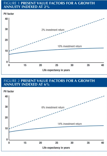
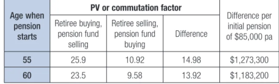
Tables 1 and 2 use Equations (3) and (3a) to summarise the PV factors for a forecast income stream when Y1 = $1 over a
range of life expectancies and expected returns. The tables assume average inflation rates of respectively 2% and 6%. In each scenario expected returns have a range of 11 percentage points starting from the given inflation rate.
TABLE 1 PRESENT VALUE FACTORS FOR A GROWTH ANNUITY COMMENCING AT $1 PER YEAR
Assumed average annual growth rate: 2%
Average net return p.a. 2% 4% 7% 10% 13%
10 9.9 9.0 7.9 6.9 6.2 15 14.9 12.9 10.6 8.9 7.6 20 19.8 16.4 12.7 10.2 8.4 25 24.8 19.6 14.4 11.1 8.9 30 29.7 22.5 15.8 11.7 9.2 35 34.7 25.1 16.8 12.2 9.4 40 39.6 27.5 17.6 12.5 9.5
TABLE 2 PRESENT VALUE FACTORS FOR A GROWTH ANNUITY COMMENCING AT $1 PER YEAR
Assumed average annual growth rate: 6%
Average net return p.a. 6% 8% 11% 14% 17%
10 9.7 8.9 7.8 6.9 6.2 15 14.6 12.7 10.5 8.9 7.6 20 19.4 16.2 12.7 10.2 8.5 25 24.3 19.4 14.4 11.2 9.0 30 29.1 22.3 15.8 11.8 9.3 35 34.0 24.9 16.9 12.3 9.5 40 38.9 27.4 17.7 12.6 9.6
By comparing Tables 1 and 2 it can be seen that, for a given life expectancy, the amount required to fund a growth annuity is dependent not so much on investment returns, but on the difference between investment returns and inflation rates. For example, a difference of 8% produces similar capitalisation factors in both inflation scenarios.
A second point worth noting is that when investment returns equal the inflation rate, capitalisation factors are a linear function of life expectancy. Thus, for example, in each table the capitalisation factors for life expectancies of 20 and 30 years are respectively exactly two and three times that for a life expectancy of 10 years when expected investment returns equal the expected inflation rate. By comparison, if investment returns exceed inflation rates by 8% in each scenario the capitalisation factors for life expectancies of 20 and 30 years are respectively approximately 48% and 70% higher than the factor for a life expectancy of 10 years. These aspects are illustrated in Figures 1 and 2.
FIGURE 1 PRESENT VALUE FACTORS FOR A GROWTH ANNUITY INDEXED AT 2%
PV factor
Life expectancy in years 40 30 20 10 0 0 15 20 25 30 35 40 10% investment return 2% investment return
FIGURE 2 PRESENT VALUE FACTORS FOR A GROWTH ANNUITY INDEXED AT 6%
PV factor
Life expectancy in years 40 30 20 10 0 0 15 20 25 30 35 40 14% investment return 6% investment return
An important conclusion to be drawn is that the most critical factor in determining the amount required to fund a growth annuity is not the duration of the annuity, but the difference between investment returns and growth rates. For example, a difference of 11 percentage points between the rates of investment returns and inflation (on which the growth rate is based) enables a lower amount to fund an
Life e xpectanc y in y ears Life e xpectanc y in y ears 27-35_Deeley_retirement.indd Sec1:30 27-35_Deeley_retirement.indd Sec1:30 5/4/07 2:04:06 PM5/4/07 2:04:06 PM
www
.finsia.ac.nz www
.finsia.edu.au
J A S S A I S S U E 1 AU T U M N 2 0 0 7 3 1
income over 40 years than would be required to fund the same income over 10 years were there no difference between the two rates. This is demonstrated in Table 3, which applies the foregoing analysis to an initial annuity of $85,000, as identified in the earlier example.
TABLE 3 CAPITAL BASE REQUIRED TO FUND A GROWTH ANNUITY COMMENCING AT $85,000 P.A.
Life expectancy
in years
Investment returns less inflation rate
0 11%
Capital base Capital base
$ x first annuity $ x first annuity
10 833,000 9.8 527,000 6.20
20 1,666,000 19.6 718,250 8.45
30 2,499,000 29.4 786,250 9.25
40 3,332,000 39.2 811,750 9.55
It should be noted that thus far capital bases have been calculated as the amount required for funding a forecast growth annuity over a given time span, at the end of which the capital base would be reduced to zero. Retirees who plan to bequeath inheritances will need to add an amount equal to the present value of planned bequests. Those planning to use retirement lump sums to pay off pre-retirement debt will also need to add an amount sufficient for the intended purpose.
PURCHASING LIFETIME INDEXED PENSIONS
The foregoing analysis is applicable to allocated and term allocated pensions, but not to the purchase of lifetime indexed pensions. Most pension funds offer lifetime indexed pensions. However, the pensions offered are typically small compared to their purchase price. For example, Table 4 summarises pertinent aspects of joint life (i.e. reversionary) lifetime indexed pensions currently offered by a pension fund.8
TABLE 4 PURCHASING A REVERSIONARY LIFETIME INDEXED PENSION Age when pension starts PV factor for annual pension Female life expectancy in years9 Implied earnings rate * % pa 55 25.9 30.25 3.985 60 23.5 25.73 3.612 65 21.0 21.39 3.035 70 18.3 17.24 2.129
*Assuming a projected inflation rate of 3% pa
Table 4 shows the implied annual earnings rate r for given life expectancies, assuming a projected inflation rate of 3%. In each case r satisfies Equation (3), as follows:
PV factor = (1 + r)0.5 × 1– 1 + (3) g n
1 + r r – g
For example, application of Equation (3) to a retirement age of 55 confirms an implied annual return rate of 3.98476% for a person with a post-retirement life expectancy of 30.25 years, as follows: (1 + r)0.5 × = PV factor1– 1 + g n 1 + r r – g
1.03984760.5 × = 25.91– 1.03 30.25 1.0398476 0.0098476
It can be seen that in all scenarios the implied rate of return is less than one percentage point above the assumed inflation rate of 3%. This leads to a conclusion that the pricing of lifetime indexed pensions, whilst to some extent driven by market forces, also reflects ultra-conservative assumptions such as low investment returns and annuitants outliving normal life expectancies (sometimes referred to as “longevity risk”).
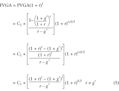
COMMUTING (i.e. SELLING) LIFETIME INDEXED PENSIONS Some superannuation schemes allow indexed pensions to be commuted into a lump sum, effectively allowing retirees to sell their indexed pensions. Table 5 compares the
commutation factors applying to the sale of indexed pensions with the PV factors applying to the purchase of indexed pensions as shown in Table 4.10
TABLE 5 PURCHASING VERSUS SELLING LIFETIME INDEXED PENSIONS Age when pension starts PV or commutation factor Difference per initial pension of $85,000 pa Retiree buying, pension fund selling Retiree selling, pension fund buying Difference 55 25.9 10.92 14.98 $1,273,300 60 23.5 9.58 13.92 $1,183,200
The significant differences between the prices at which pension funds buy and sell indexed pensions suggest that pension broking is potentially extremely profitable. The data also suggest that lifetime indexed pensions are typically too expensive to buy and too valuable to commute (i.e. sell). In all cases rates of return implied by commuting a reversionary indexed pension are more than 10% above the inflation rate and therefore unlikely to be achieved. The conclusion is that pensioners with at least normal life expectancies are better off retaining their pensions than commuting them.
EVALUATING AND CONSTRUCTING A RETIREMENT SAVINGS PLAN
The adequacy of a retirement savings plan can be assessed in terms of the extent to which it will achieve the capital base required to fund post-retirement cash flows. This involves calculating the combined future value of current savings and
27-35_Deeley_retirement.indd Sec1:31
www
.finsia.edu.au www
.finsia.ac.nz
J A S S A I S S U E 1 AU T U M N 2 0 0 7 3 2
the savings plan. The future value of current savings can be defined as follows:
FVt = S(1 + r)t (4)
where FVt = the future value of current savings
S = current savings.
If periodic savings are assumed to increase in line with income growth, they have the form of a growth annuity, the future value of which can be defined as follows:
FVGA = PVGA(1 + r)t = C1 × (1 + 1– 1 + r)t+0.5 g
'
t 1 + r r – g'
= C1 × (1 + r)t+0.5 (1 + r)t – (1 + g
'
)t (1 + r)t r – g'
= C1 × (1 + r)0.5 r ≠ g'
(5) (1 + r)t – (1 + g'
)t r – g'
where C1 = the current annual contribution to a retirement
savings plan net of any applicable contribution tax. As with Equation (3), Equation (5) cannot provide a solution when r = g
'
, in which case:FVGA = C1 × t(1 + g
'
)t-0.5 = C1 × t(1 + r)t-0.5 (5a)Table 6 summarises the future values of annual savings commencing at $1, given a forecast growth rate of 5% and a range of annual net rates of return.
TABLE 6 FUTURE VALUE FACTORS FOR A GROWTH ANNUITY COMMENCING AT $1 PER YEAR
Assumed average annual growth rate: 5%
Average net return p.a. 5% 7% 10% 13% 16%
5 6.2 6.5 7.0 7.5 8.1 10 15.9 17.5 20.2 23.5 27.2 15 30.4 35.2 44.0 55.5 70.4 20 51.8 62.9 85.5 117.9 164.6 25 82.6 105.6 156.2 237.1 367.1 30 126.5 170.2 275.4 462.3 798.3 35 188.4 266.9 473.8 884.3 1,711.5 40 274.8 410.4 801.7 1,670.8 3,639.2
The combined future value of current savings and a savings plan can now be defined as follows:
ΣFV = S(1 + r)t + C1 × (1 + (1 + r)t – (1 + g
'
)t r)0.5 (6)r – g
'
where ΣFV = the combined future value of current savings and a savings plan.
The adequacy of that future value to meet post-retirement cash flows can be evaluated by subtracting the capital base defined by Equation (3). Positive and negative differences respectively indicate adequacy or inadequacy.
A positive difference indicates that contributions within an existing savings plan are more than sufficient to generate the required capital base. There will also be occasions when current savings appear high enough to obviate the need for further contributions. In either scenario it is recommended that contributions to retirement savings plans be maintained so long as they are tax-effective. In any event, salary
packaging of superannuation mandates contributions irrespective of expectations of future wealth.
In the event of a predicted funding shortfall, additional savings required to fund the deficit can be defined as follows:
C'1 = – (funding deficit) × (1+r)t–(1+g
'
)t r–g'
× (1+r)
–0.5
1–ct (7)
where C'1 = required additional periodic savings before applicable
superannuation contribution tax
funding
deficit = FV of savings less required capital base
= S(1+r)t+ (1+r) t – (1+g
'
)t r – g'
(1+r) 0.5–Y 1(1+r)0.5 1– 1+g n 1+r r–gct = applicable contribution tax.
Equation (7) can be used as the basis for a spreadsheet-based retirement planning model, as demonstrated in the following comprehensive example.
COMPREHENSIVE EXAMPLE
An employee plans to retire in five years. Current gross annual income and savings are respectively $90,000 and $360,000. Projected average annual rates of inflation, income growth and investment net returns are respectively 3%, 4% and 11%. Compulsory employer and employee super annuation contributions are respectively 17% and 8.25% of gross annual income. Tax-deductible and non-tax-deductible work-related expenses are currently $1,500 and $2,400 respectively. Life expectancy at time of retirement is assumed to be 24 years. Pension payment fees are currently $150 per year. Super-annuation contribution tax is payable at the rate of 15% and personal tax rates are as for 2006–07. A Medicare levy is payable at the rate of 1.5% of taxable income.
Years to r
etir
ement
27-35_Deeley_retirement.indd Sec1:32
www .finsia.ac.nz www .finsia.edu.au J A S S A I S S U E 1 AU T U M N 2 0 0 7 3 3 = $360,000 × 1.115 + $19,316.25 × 1.11 5 – 1.045 0.07 × 1.11 0.5 = $742,799
Step 5: Determine adequacy of existing savings Surplus/deficit = Future value of savings less required capital base
= $742,799 − $765,911 = −$23,112
Step 6: Determine additional savings required to fund the identified deficit
C'1 = –($23,112) × (1+r)t–(1+g
'
)t r–g'
× (1+r) –0.5 1–ct (7) = $23,112 × 1.115 – 1.045 0.07 × 1.11–0.5 1– 0.15 = $23,112 × 0.166876763 = $3,857 p.a. = $148 per fortnightStep 7: Determine the annual amount of income tax and Medicare levy avoided by making additional superannuation contributions from pre-tax income
Amount saved = $3,857 × 0.415
= $1,601
Spreadsheet solution
The complexity of the foregoing calculations can be avoided by using an appropriate spreadsheet model. Appendix A demonstrates such a model, which is applied to the foregoing example.
SUMMARY
This article has presented retirement planning as a three-step process involving the forecasting of post-retirement cash flow needs, determining the composition and value of a capital base sufficient to fund those cash flows, and identifying a retirement savings plan aimed at achieving the required capital base. Each step benefits from the application of mathematical routines that can be combined into a composite spreadsheet-based model aimed at
enhancing and facilitating the retirement planning process. It can also be shown that, from the retiree’s point of view, lifetime indexed pensions are likely to be overpriced when buying and underpriced when selling (i.e. commuting to a lump sum).
Readers may request a copy of the spreadsheet model from the author at [email protected]
Are the employee’s savings and savings plan sufficient to ensure, within the model’s parameters, that existing living standards, based on current net disposable income, can be maintained throughout retirement? If not, what additional superannuation contributions should be made per fortnight and how much would those additional contributions, if required, save annually on income tax and Medicare levy? SOLUTION
Step 1: Calculate the income required in the
first year of retirement (Y1)
Current gross annual income $90,000 Less pre-tax superannuation contributions $7,425
tax-deductible expenses 1,500
89,250
Taxable income 81,075
Less income tax 20,280
Medicare levy 1,216
non-tax-deductible work-related expenses 2,400
23,896
57,179
Y1 = $57,179 × (1.04)5 + $150 × (1.03)5 = $69,740.89.
Step 2: Calculate the capital base needed to fund post-retirement cash flows
Required capital base = Y1(1 + r)0.5 ×
1– 1 + g n 1 + r r – g
(3) = $69,740.89 × 1.110.5 × 1– 1.03 24 1.11 0.08
= $765,911
Step 3: Calculate value of current superannuation
contributions net of contribution tax (C1)
C1 = $90,000 × (0.17 + 0.0825) × 0.85
= $19,316.25
Step 4: Calculate the future value of current savings
and savings plan (ΣFV)
ΣFV = S(1+r)t + C1 × (1+r) t – (1+g
'
)t r – g'
(1+r) 0.5 (6) 27-35_Deeley_retirement.indd Sec1:33 27-35_Deeley_retirement.indd Sec1:33 5/4/07 2:04:08 PM5/4/07 2:04:08 PMwww
.finsia.edu.au www
.finsia.ac.nz
J A S S A I S S U E 1 AU T U M N 2 0 0 7 3 4
RETIREMENT PLANNING TEMPLATE
I N P U T O U T P U T
Enter male (M) or female (F) Years to retirement
Indicative return on investment
Current age Life-expectancy at retirement
Planned age at retirement
Compulsory employee super contributions Pension required in first year of retirement
Current annual salary
Forecast income growth rate Taxable income FV required on retirement
Employee super contrib. rate Income tax payable FV of current savings
Employer super contrib. rate Medicare levy payable FV of super
Additional employee super * *Tax and Medicare levy saved Total FV
Medicare levy rate After-tax income FV surplus/deficit
Contribution tax rate Disposable income# Additional savings required?
Tax-deductible expenses Compulsory employer super contributions Additional super contributions pa
Other work-related expenses Total super contributions less contribution tax Additional super contributions per fortnight
Current savings (capital) # Enter disposable income in cell immediately to the right when there is a funding deficit.
Forecast inflation rate Investment risk: hi, med or lo Alternative life expectancy Annual pension payment fee
References
Australian Bureau of Statistics (2006), Life Tables, Australia, 2003–2005, Canberra.
Bateman H., (2006), ‘Recent Superannuation Reforms: Choice and Flexibility in Retirement’, Australian Accounting Review, Vol. 16, No. 3, pp 2–6.
Bateman H., Kingston G. and Piggott J., (2001), ‘Forced Saving: Mandating Private Retirement Incomes’, Cambridge University Press.
Bridges Personal Investment Services (2006), unpublished seminar papers on the “old” NSW State Superannuation Scheme, Sydney.
Drew, M.E., and Stanford, J.D., (2003), ‘Principal-and-Agent Problems in Superannuation Funds.’ Australian Economic Review, Vol. 36, No. 1, March, pp 98–107.
Drew, M.E., Stanford, J.D. and Stanhope, B., (2005),
‘Sustainable Retirement: A Look at Consumer Desires’, Australasian Journal of Business and Social Enquiry, Vol. 3, No. 3, pp 1–23.
Gallery, G., Gallery, N. and Brown, K., (2004),
‘Superannuation Choice: The Pivotal Role of the Default Option’, Journal of Australian Political Economy, 53, pp 44–66.
Martin P. and Burrow M., (1991), Applied Financial Mathematics, Prentice Hall, Sydney.
UniSuper 2006, Looking Forward: Your Guide to Pension Choices in Unisuper, Sydney.
UniSuper 2006, survey results located at: www.unisuper. com.au/resources/News/feature, accessed on 17 January 2007.
Notes
1 These are the results of a UniSuper survey as reported at www.unisuper.com.au/resources/News/feature, accessed on 17 January 2007.
2 See Bateman (2006) and Bateman, Kingston and Piggott (2001). 3 See Drew and Stanford (2003).
4 See Drew, Stanford and Stanhope (2005). 5 See Gallery, Gallery and Brown (2004)
6 The writer has to date located no Australian financial mathematics text that provides derivations of PVGA and/or FVGA equations. One text includes a page on the future value of growth annuities (plus one end-of-chapter problem) with no derivation and no mention of the present value of growth annuities. See Martin P. & Burrow M., (1991), Applied Financial Mathematics pp 67–68.
7 The analyses demonstrated in this paper assume that pensions paid (to retirees aged 60 and over) after 1 July 2007 will be tax-exempt and therefore not subject to the Medicare levy. 8 The pension fund is UniSuper. The figures in Table 4 are adapted from details provided on pages 19 and 37 of Looking Forward: Your Guide to Pension Choices in UniSuper, 2006. 9 Sourced from Life Tables, Australia, 2003–2005, Australian Bureau of Statistics, 2006.
10 The commutation factors shown in Table 5 are those applying to reversionary indexed pensions offered by the “old” NSW State Superannuation Scheme, which closed to new members on 30 June 1985.
APPENDIX A
27-35_Deeley_retirement.indd Sec1:34
www
.finsia.ac.nz www
.finsia.edu.au
J A S S A I S S U E 1 AU T U M N 2 0 0 7 3 5
RETIREMENT PLANNING TEMPLATE: SHOWING FIRST STAGE OF DATA ENTRY
I N P U T O U T P U T
Enter male (M) or female (F) M Years to retirement 5
Indicative return on investment 11.00%
Current age 60 Life-expectancy at retirement 18.13
Planned age at retirement 65 Compulsory employee super contributions 7,425 Pension required in first year of retirement 69,741
Current annual salary 90,000 Taxable income 81,075 FV required on retirement 765,911
Forecast income growth rate 4.00% Income tax payable 20,280 FV of current savings 606,621
Employee super contrib. rate 8.25% Medicare levy payable 1,216 FV of super 136,178
Employer super contrib. rate 17.00% *Tax and Medicare levy saved Total FV 742,799
Additional employee super * After-tax income 59,579 FV surplus/deficit -23,110
Medicare levy rate 1.50% Disposable income# 57,179 Additional savings required? YES
Contribution tax rate 15.00% Compulsory employer super contributions 15,300 Additional super contributions pa 3,857
Tax-deductible expenses 1,500 Total super contributions less contribution tax 19,316 Additional super contributions per fortnight 148
Other work-related expenses 2,400 # Enter disposable income in cell immediately to the right when there is a funding deficit.
Current savings (capital) 360,000
Forecast inflation rate 3.00%
Investment risk: hi, med or lo hi
Alternative life expectancy 24
Annual pension payment fee 150.00
RETIREMENT PLANNING TEMPLATE: SHOWING SECOND & FINAL STAGE OF DATA ENTRY
I N P U T O U T P U T
Enter male (M) or female (F) M Years to retirement 5
Indicative return on investment 11.00%
Current age 60 Life-expectancy at retirement 18.13
Planned age at retirement 65 Compulsory employee super contributions 7,425 Pension required in first year of retirement 69,741
Current annual salary 90,000 Taxable income 77,218 FV required on retirement 765,911
Forecast income growth rate 4.00% Income tax payable 18,737 FV of current savings 606,621
Employee super contrib. rate 8.25% Medicare levy payable 1,158 FV of super 159,291
Employer super contrib. rate 17.00% *Tax and Medicare levy saved 1,601 Total FV 765,912
Additional employee super * 3,857 After-tax income 57,323 FV surplus/deficit 1
Medicare levy rate 1.50% Disposable income# 57,179 54,923 Additional savings required? NO
Contribution tax rate 15.00% Compulsory employer super contributions 15,300 Additional super contributions pa Not applicable
Tax-deductible expenses 1,500 Total super contributions less contribution tax 22,595 Additional super contributions per fortnight Not applicable
Other work-related expenses 2,400 # Enter disposable income in cell immediately to the right when there is a funding deficit.
Current savings (capital) 360,000
Forecast inflation rate 3.00%
Investment risk: hi, med or lo hi
Alternative life expectancy 24
Annual pension payment fee 150.00
27-35_Deeley_retirement.indd Sec1:35