Understanding Exchange Rate Dynamics: What Does
The Term Structure of FX Options Tell Us ?
Yu-chin Chen and Ranganai Gwati
∗December 2014
Abstract
This paper uses foreign exchange (FX) options with different strike prices and maturities (“the term structure of volatility smiles”) to capture both market expectations and perceived risks. Using daily options data for six major currency pairs, we show that the cross section and term structure of options-implied standard deviation, skewness and kurtosis consistently explain not only the conditional mean but also the entire conditional distribution of subsequent currency excess returns for horizons ranging from one week to twelve months. We also find that exchange rate movements, which are notoriously difficult to model empirically, are in fact well-explained by the term structures of forward premia and options-implied higher moments. The robust empirical pattern is consistent with a representative expected utility maximizing investor who, in addition to the mean and variance, also cares about higher moments in the return distribution. The term structure linkage in turn provides support for an Epstein-Zin type preference. Our results suggest that the perennial problems faced by the empirical exchange rate literature are likely due to overly restrictive assumptions inherent in the prevailing testing methods, which fail to properly account for the forward-looking property of exchange rates and potential skewness or excess kurtosis in the conditional distribution of FX movements.
Keywords: exchange rates; excess returns; options pricing; volatility smile; risk; term structure
of implied volatility; quantile regression
JEL Code: E58, E52, C53,F31,G15
∗First Draft:October 2012. We are indebted to the late Keh-Hsiao Lin and Joe Huang for pointing
us to the relevant data sources. We would also like to thank Samir Bandaogo, Nick Basch, Yanqin Fan, David Grad, Ji-Hyung Lee, Charles Nelson, Bruce Preston, Abe Robison, and Eric Zivot for their helpful comments and assistance. All remaining errors are our own. Chen’s and Gwati’s research are supported by the Gary Waterman Scholarship and the Buechel Fellowship at the University of Washington. Chen:
1
Introduction
The exchange rate economics literature has over the years faced many empirical puzzles. As an example, although theory predicts that nominal exchange rates should depend on current and expected future macroeconomic fundamentals, the consensus in the literature is that exchange rates are essentially empirically “disconnected” from the macroeconomic variables that are supposed to determine them. This empirical disconnect comes in the form of low correlations between nominal exchange rates and their supposed macro-based determinants and also in the form of poor performance of macro-based exchange rate models in out-of-sample forecasting.1
A related empirical anomaly that has received considerable attention in the literature is the uncovered interest parity (UIP) puzzle or the forward premium puzzle. The UIP puzzle is the empirical irregularity showing that the forward exchange rate is a biased predictor of future spot exchange rates. The UIP puzzle is taken seriously in the exchange rate literature because the UIP condition is a property of most open-economy macroeconomic models.
One manifestation of this empirical (ir)regularity is that countries with higher interest rates tend to see their currencies subsequently appreciate and a “carry-trade” strategy exploiting this pattern, on average, delivers excess currency returns.2 This violation of the UIP condition is commonly attributed to time-varying risk premia and biases in (measured) market expectations. However, empirical proxies based on surveyed forecasts or standard measures of risk - for instance, ones built from consumption growth, stock market returns,
or the Fama and French (1993) factors -have been unsuccessful in explaining the puzzle.3As
such, while recognizing the presence of risk, macroeconomic-based approaches to modeling
1 See Engel (2013) for a review.
2 A carry trade strategy is to borrow low-interest currencies and lend in high-interest currencies, or to
sell forward currencies that are at a premium and buy forward currencies with a forward discount.
3See, Engel (1996) for a survey of the forward premium literature, as well as recent studies such as
exchange rates often ignore risk in empirical testing.4 5
This paper argues that the persistent empirical puzzles faced by the exchange rate economics literature are most likely due overly restrictive preference and distributional assumptions in conventional testing methods. For example, researchers typically assume that exchange rate returns are normally distributed, or that investors’ utility functions depend only on the mean and variance. We argue that these auxiliary assumptions often inadequately account for either the forward-looking property of nominal exchange rates or potential skewness and/or fat tails in the distribution of FX returns.
We empirically demonstrate that FX risks as captured by higher order moments of perceived FX returns distributions of perceived FX return distributions, as well as expectations, captured by the term structure of option prices, do really matter in explaining exchange rate movements. We highlight the usefulness of capturing risks and expectations in stages. First, we show that options-implied standard deviations, skewness and kurtosis of future exchange rate movements are able to explain not only the conditional mean, but the entire conditional distribution of excess currency returns. Second, we show that information extracted from the term structure options-implied risk measures add substantial explanatory power for excess currency returns. Finally, we show that quarterly exchange rate movements are well explained by the term structure of 1st-4thmoments of options-implied returns distributions,
with adjusted R2s ranging from 58% for USDJPY to 84% for GBPUSD.
Simple derivatives such as the forwards and futures have been used extensively in explaining
excess currency returns or exchange rate movements.6 Payoffs from forward contracts,
however, are linear in the return on the underlying currency and as such do not contain as
4 ( See for instance, Engel and West (2005); Mark (1995))
5On the finance side, efforts aiming to identify portfolio return-based “risk factors” offer some empirical
success in explaining the cross-sectional distribution of excess FX returns, but have little to say about bilateral exchange rate dynamics (see for example, Lustig et al. (2011); Verdelhan (2012)). Lustig et al. (2011) and Verdelhan (2012) for example, identify a “carry factor” based on cross sections of interest rate-sorted currency returns and a “dollar factor” based on cross sections of beta-sorted currency returns.
useful a set of information as the non-linear contracts we examine. Conceptually, since payoffs of option contracts depend on the uncertain future realization of the price of the underlying asset, option prices must reflect market sentiments and beliefs about the probability of future payoffs.
Our use of options price data and related empirical methodologies has a number of motivating factors. First, options are forward-looking by construction, which means option prices should therefore be able to incorporate information such as forthcoming regime switches
or the presence of a peso problem.7 Second, option prices are deeply rooted in market
participant behavior because they are based on what market participants do instead of what they say.Furthermore, cross sections of option prices imply a subjective probability distribution of future spot exchange rates, which captures both market participants’ beliefs
and preferences. 8Third, modern techniques such as the Vanna-Volga method 9 and the
methodology of Bakshi et al. (2003) facilitate elegant and model-free computation of options-implied higher order moments of future exchange rate changes.
Our empirical findings in this paper have three implications. First, the exchange rate model based on UIP is not that bad, and we can continue using it in open economy macroeconomic models. However, we need to understand that if we put lognormal shocks, they will not fit will. Quick improvements can be made by controlling for the term structure of higher order moments, which can be obtained from option price data. Second, on the financial side, concepts of risk which depend on only the mean and variance such as the Sharpe ratio for portfolio performance evaluation, perhaps ought to be modified to account for the importance of higher moment risks such as skewness and kurtosis.
7 The peso problem refers to the effects on inferences caused by low-probability events that do not occur
in the sample, which can lead to positive excess return.
8This distribution is commonly referred to as the “risk-neutral distribution”, though it does NOT
imply that the distribution is derived under risk-neutrality. On the contrary, it incorporates both the expected physical probability distribution of future exchange rate realization as well as the risk premium, or compensation required to bear the uncertainty.
2
Why Higher Order Moments and Term Structure?
2.1
Forward Premium Puzzle and Excess Currency Returns
The efficient market condition for the foreign exchange markets, under rational expectations, equates cross border interest differentials it−i∗t with the expected rate of home currency
depreciation, adjusted for the risk premium associated with currency holdings, ρt:10
iτt −iτ ,t ∗ =Et∆st+τ +ρt+τ. (2.1)
This condition is expected to hold for all investment horizons τ, with interest rates that are
at matched maturities. Ignoring the risk premium term, numerous papers have tested this
equation since Fama (1984), and find systematical violations of this UIP condition:
st+τ −st =α+β(iτt −i
∗,τ
t ) +t+τ; Et[t+τ] = 0,∀t,
H0 :β = 1
(2.2)
with an estimated β < 0 and R2s that are usually close to zero. This is the so-called
uncovered interest rate parity puzzle or the forward premium puzzle (see Engel (1996), for a survey of the literature). To see the connection with forward rates, we note that the covered interest parity condition, an empirically valid no-arbitrage condition, equates the forward premiumftt+τ−st,with interest differentials. The risk-neutral UIP condition above
thus implies that the forward rate should be an unbiased predictor for future spot rate:
Etst+τ =ftt+τ or st+τ =ftt+τ +ut+τ,where Et[ut+τ] = 0∀t.
We should next define FX excess returns as the rate of return across borders net of currency movement, and one can see that the UIP or forward premium puzzle can be
10 In this paper, we define the exchange rate as the domestic price of foreign currency. A rise in the
exchange rate indicates a depreciation of the home currency. However, “home”does not have a geographical significance but follow the FX market conventions. See table (1A)
expressed as a non-zero averaged excess return over time:
xrt+τ =ftt+τ −st+τ = (iτt −i τ ,∗
t )−∆st+τ =ρt+τ +ut+τ (2.3)
It is natural then to note that the empirical failure of the risk-neutral UIP condition can be attributable to either the presence of a time-varying risk premium, ρt+τ, or that expectation
error, ut, may not be i.i.d. mean zero over time. If the distribution of either of these is
not mean zero over the time series, empirical estimates of the slope coefficient in regression equation (2.2) would likely suffer omitted variable bias or other complications.
2.2
Why higher order moments?
11We show that in addition to risk neutrality and rational expectations assumptions, the UIP condition also hinges on the rather restrictive auxiliary assumptions that FX returns are i.i.d. normal over time and that investors have constant absolute risk aversion (CARA) utility. The two additional assumptions have the effect of reducing the representative investor’s optimal asset allocation problem to a mean-variance optimization problem.
We start with the problem of an investor who, in each period, allocates her portfolio among risky assets with the goal of maximizing the expected utility of next period wealth. In each period, the investor hasn risky assets to choose from. The vector of gross returns is given byrt+1 = (r1,t+1, ..., rn,t+1). If we supposeWtis arbitrarily set to 1, thenWt+1 =α
0
trt+1 , where α is an n by 1 vector of portfolio weights.
The investors problem is to choose αt to maximize the expression
Et[U(Wt+1)] =Et[U(α 0 trt+1)] =R ...R U(Wt+1)f(rt+1)dr1,t+1dr2,t+1...drn,t+1 (2.4)
subject to the condition thatPn
i=1αi,t = 1, wheref(rt+1) is the joint probability distribution
of rt+1.
2.2.1 CARA and Normality reduce problem to mean-variance optimization
Let us further assume that the investor has CARA utility and that returns are conditionally normally distributed. The CARA utility assumption means the utility is given by
U(Wt+1) = −e−γWt+1 , where γ ≥ 0 is the coefficient of absolute risk aversion. The distributional assumption rt+1 ∼N(µt+1,Σt+1) implies that Wt+1 ∼N(µp,t+1, σ2p,t+1), where
µp,t+1 =α0tµt+1 and σ2p,t+1 =α0tΣt+1αt
With the above two assumptions, expression (2.4) reduces to12
Et[U(Wt+1)] = −Et[e−γWt+1] =γµp,t+1− 1 2γ
2σ2
p,t+1 (2.5)
Equation (2.5) demonstrates that under the assumptions of CARA utility function and conditional normality of returns, the general portfolio allocation problem (2.4) reduces to
the mean-variance optimization problem.13
If we further assume that our investor has a 2-asset portfolio made up of a nominally
safe domestic bond and a foreign bond, and that she allocates a fraction α of her wealth to
the domestic bond, then next period wealth expressed in local currency units is given by
Wt+1 = α(1 +it) + (1−α)(1 +i∗t) St+1 St. Wt (2.6)
In this 2-asset example and CARA utility and conditionally normal returns the expressions
12The second equality follows from the fact that e−γWt+1 ∼ LN(−γµ
p,t+1, γ 2σ2
p,t+1) , so Et[e−γWt+1] =
−γµp,t+1+γ2σ2p,t+1
13The quadratic utility function imply mean variance optimization for arbitrary return distribution.
However, the quadratic utility implies increasing absolute risk aversion and satiation (Jondeau et al. (2010), page 352).
for the conditional mean and variance of next period wealth are given by: µp,t+1 = h α(1 +it) + (1−α)(1 +i∗t)E tSt+1 St i Wt, σ2 p,t+1 = (1−α)2(1+i∗ t)2V art(St+1)Wt2 S2 t (2.7)
Plugging the expressions in equation (2.7) into objective function (2.5), taking the first order condition with respect toαand rearranging the first order condition yields the following
equation which implicitly determines the optimal α:
(1 +it)−(1 +i∗t) EtSt+1 St = −γWt(1−α)(1 +i ∗ t)2V art(St+1) S2 t . (2.8)
Equation (2.8) reduces to the UIP condition if we assume that all investors are risk-neutral (γ = 0):14 1 +it 1 +i∗t = EtSt+1 St . (2.9)
The Fama regression in equation (2.2) tests a logarithmic version of equation (2.9). The key steps in deriving the testable restrictions in equation (2.9) are the joint assumptions of CARA utility and conditional normality of next period wealth, which reduce the investor’s
optimization to mean-variance. The above discussion illustrates that deriving the UIP
equation tested through expression (2.2) depends on other assumptions beyond rational
expectations and risk-neutrality. If the normality assumption is dropped, for example, then expression (2.9) will most likely include higher order moments. In fact, Jondeau et al. (2010) note that under CARA utility, if we drop the normality assumptions, then the investor would prefer positive skewness and low kurtosis, such that the investor’s objective function in equation (2.5) will also include the third and fourth moments of the FX return distribution. Scott and Horvath (1980) show that a strictly risk-averse individual who always prefers more to less (U(1) >0) and likes positive skewness at all wealth levels will necessarily dislike high
kurtosis.
2.2.2 Asset allocation under higher order moments15
We showed in subsection (2.2) that the assumptions of CARA utility and normality of returns reduce the investor’s problem to mean-variance optimization. However, if the distribution of portfolio returns is asymmetric, or the investor’s utility function is of a higher order than the quadratic, or the mean and variance do not completely determine the distribution of asset returns, then higher order moments and their signs must be taken into account in the portfolio asset allocation problem. In this subsection we present a framework for incorporating higher order moments into the asset allocation problem.
The objective in (2.4) can be intractable and it is usual to focus on approximation of (2.4) based on higher order moments. Jondeau et al. (2010) consider a Taylor’s series expansion of the utility function around expected utility up to the fourth order:
U(Wt+1) = U(EtWt+1) +U(1)(Wt+1)(Wt+1−EtWt+1) + 2!1U(2)(Wt+1)(Wt+1−EWt+1)2+ 1 3!U (3)(W t+1)(Wt+1−EtWt+1)3+4!1U(4)(Wt+1)(Wt+1−EtWt+1)4, (2.10) where Un(.) denotes the nth derivative of the utility function with respect to next period
wealth. Taking the conditional expectation of expression ( 2.10) yields
Et[U(Wt+1)]≈U(EtWt+1) +U(1)(Wt+1)(Wt+1−EtWt+1) + 2!1U(2)(Wt+1)(Wt+1−EtWt+1)2+ 1 3!U (3)(W t+1)(Wt+1−EtWt+1)3+4!1U(4)(Wt+1)(Wt+1−EtWt+1)4. (2.11) Under the assumption that the investor’s utility function is CARA, expression (2.11) reduces to Et[U(Wt+1)]≈ −e−γµp h 1 + γ22σ2 p− γ3 6 s 3 p+ γ4 24k 4 p i . (2.12)
In equation (2.12),s3pandk4p are the skewness and kurtosis of portfolio return. It is clear from equation (2.12) that under CARA utility, investors prefer positive skewness and dislike high variance and high kurtosis. Optimal portfolio weights can then be obtained by maximizing expression (2.11) instead of the exact objective function shown in expression (2.4).
For CARA utility, the weight the investor puts on the higher order moments depends
on the degree of risk aversion parameter γ. In more general settings, however, the weight
on the nth moment depends on the nth derivative of the utility function, and the signs of
sensitivities of utility function to changes in higher moments cannot be easily pinned down. If the moments are not orthogonal to each other, then the effect of utility of increasing one moment might not be straight forward. Scott and Horvath (1980) establish some general conditions for investor preference for skewness and kurtosis.
2.3
Why term structure of option-implied moments?
Rearranging the UIP relationship in equation (2.1) and iterating forward, we can show that the nominal exchange rate depends on current and expected future interest rate differentials as well as on expected future risk:
st= − ∞ X j=0 Et(it+j −i∗t+j) | {z }
Expected future interest differentials
− ∞ X j=0 Etρt+j | {z } Expected Future FX risk
(2.13)
Expression (2.13) highlights the link between the exchange rate and macroeconomic fundamentals. There is a huge literature linking the term structure of interest rate rates(yield curve) to expected future dynamics of macroeconomic fundamentals such as monetary policy, inflation and output by observing that short term interest rates are monetary policy variables that depend on macroeconomic variables such as inflation and output while longer term yields
are risk-adjusted averages of expected future short rates.16 Chen and Tsang (2013) extend
this strand of literature to the open economy context by noting that the term structure of interest rate differentials (relative yield curve) contain information about the expected future dynamics of differences in macroeconomic fundamentals. We note that the relative yield curve captures the same information about expected macroeconomic fundamentals as
the term structure of option-implied first moments of future exchange rate movements. We
extend the literature on yield curve-exchange rate linkage by investigating the ability of entire option-implied distributions to explain exchange rate dynamics.
Writing the exchange rate in the form in equation (2.13) also demonstrates the importance of capturing expectations and risk in the empirical modeling of exchange rate. Standard empirical approaches usually impose distributional assumptions that reduce the sum of
expected future fundamentals to equal current fundamentals and also ignore risk. 17
There is also a strand of literature that document the empirical success of empirical exchange rate models that capture information in the term structure of forward premia.Clarida and Taylor (1997) and Clarida et al. (2003) show that even if the forward rate is a biased predictor of future spot rate (the forward premium puzzles),the term structure of forward premia still contains information useful for predicting subsequent exchange rate changes. This line of literature is linked to Chen and Tsang (2013) by observing that through the empirically valid covered interest parity (CIP) condition, the forward premium equals the interest rate differential at all maturities.
3
Information Content of Currency Options
3.1
Volatility Smile and Term Structure of Option Prices
Breeden and Litzenberger (1978) show that in complete markets, the call option pricing
function (C) and the exercise price K are related as follows:
∂2C
∂K2 =e
−rdτ
πQt (St+τ), (3.1)
where rd and rf are the domestic and foreign risk-free interest rates and πQ
t(St+τ) is the
risk-neutral probability density function (pdf) of future spot rates. Equation (3.1) implies that, in principle, we can estimate the whole pdf of time St+τ spot exchange rate from time
t volatility smile. Once the distribution is available, it becomes possible to get empirical
estimates of the standard deviation, skewness , kurtosis and even higher order moments of the market perceived probability density of St+τ given information available at timet.
In addition to the Breeden and Litzenberger (1978) result in equation (3.1), we note that although market participants can be treated as if they are risk-neutral for the purpose of option-pricing, option prices theoretically contain information about both investor beliefs and risk preferences, as shown from the following formula for the price of a European-style call option: C(t, K, T) = Z ∞ K Mt,T(ST −K) | {z } Preferences πPt (ST) | {z } Beliefs dST =e−r dτZ ∞ K (ST −K)πQt (ST) | {z } Both dST. (3.2)
In equation (3.2),Mt,t+τ is the pricing kernel, which captures the investor’s degree of risk
aversion and πPt(St+τ) is the physical probability density function of future spot exchange
rates 18.
A forward contract can in fact be viewed as a European-style call option with a strike price of zero. To see this, we recall that, on one hand, the theoretical forward exchange rate is given by the formula:
18 In the second expression, the pricing kernel is performing both the risk-adjustment and discounting
Ft,T =e−r dτZ ∞ 0 STπQt (ST)dST =e−r dτ EQt(ST). (3.3)
On the other hand, evaluating equation (3.2) at K=0 yields:
C(t,0, T) = e−rdτ
Z ∞
0
STπQt(ST)dST =Ft,T. (3.4)
The relationship between options and forwards in equation (3.4) suggests that the cross section of option prices should, at a minimum, contain as much information about investor beliefs and preferences as that contained in forward prices.
Moving on to the term structure of option prices, one way to motivate the theoretical information content of the term structure of option prices is to start from equation (2.13):
st = − ∞ X j=0 Et(it+j −i∗t+j) | {z }
Expected future interest differentials
− ∞ X j=0 Etρt+j | {z } Expected Future FX risk
. (3.5)
Now, under the empirically valid CIP condition, interest rate differential is equal to the forward premium for all tenors j:19
it+j−i∗t+j =f t+j t −st=−rdτ +EtQ ln St+j St | {z } First moment ofπQt + ωt |{z} Jensen’s inequality term
,∀ tenor j. (3.6)
Equation (3.6) thus says that, ignoring the Jensen’s inequality termωtand the constant
term −rdτ, the interest rate differential equals the first moment of the option-implied
risk-neutral distribution of lnSt+j
St
for any given tenorj. The interest rates are monetary
policy variables and therefore depend on macroeconomic fundamentals such as unemployment
19The second equality follows from dividing (3.3) by S
and inflation. When combined, equations (3.6) and (3.5) demonstrate that just like the yield curve, the term structure of the first moments of implied distributions also captures
information about current and expected future macroeconomic fundamentals.
A second motivation for the information content of the term structure of option prices comes from the expectation hypothesis for implied volatility,that the term structure of option-implied volatility contain information about the market’s perception about the future dynamics of short term implied volatility. If the expectations hypothesis holds in the FX market, then the implied volatility for long dated options should be consistent with the
implied volatility of short dated options quoted today and in the future. 20
3.2
Extracting Option-Implied Moments
We use the methodology of Bakshi et al. (2003) (henceforth BKM) to extract model-free option-implied standard deviation, skewness and kurtosis from the volatility smile. Grad (2010) and Jurek (2009) also use the BKM methodology to extract FX options-implied
higher order moments. 21 The BKM methodology rests on the results of Carr and Madan
(2001), which show that if we have an arbitrary claim with a pay-off function H[S] with finite expectations, then H[S] can be replicated if we have a continuum of option prices. They also show that if H[S] is twice-differentiable, then it can be spanned algebraically by the following expression H[S] = (H[ ¯S] + (S−SH¯ S[ ¯S]) + Z ∞ ¯ S HSS[K](S−K)++ Z S¯ 0 HSS[K](K−S)+dK, (3.7)
20For example, if the current six month implied volatility is 10% and the current three month implied
volatility is 5%, then, under the expectation hypothesis, then the three month implied volatility three months from now should be 13.2% because
0.5(0.1)2= 0.25(0.05)2+ 0.25(0.132)2.
where HS = ∂H∂S and HSS = ∂
2H
∂S2. Assuming no arbitrage opportunities, the price of a claim
with pay-off H[S] is given by the expression
pt= (H[ ¯S]−SH¯ S[ ¯S])e−r dτ +HS[ ¯S]Se−r dτ + Z ∞ ¯ S HSS[K]C(t, τ , K)+ Z S¯ 0 HSS[K]P(t, τ , K)dK (3.8) where K is the strike price, C(t, τ , K) and P(t, τ , K) are, respectively, the prices of a
European-style call and put options. ¯S is some arbitrary constant, usually chosen to equal
current spot price.
Equation (3.8) indicates that any pay-off function H[S] can be replicated by a position of (H[ ¯S]−SH¯ S[ ¯S]) in the domestic risk-free bond, a position of H[ ¯S] in the stock, and
combinations of out-of-the-money calls and puts, with weights HSS[K]. Suppose we have
contracts with the following pay-off functions:22
H[S] = [Rt(St+τ)]2, Volatility Contract [Rt(St+τ)]3, Cubic Contract [Rt(St+τ)]4, Quartic Contract, (3.9) where Rt(St+τ) = ln(StS+tτ
. BKM show that the variance, skewness and kurtosis of the
distribution of Rt+τ can be calculated using the following formulas:
Stdev(t, τ) =perdτ V(t, τ)−µ(t, τ)2 (3.10a) Skew(t, τ) = erdτW(t,τ)−3V(t,τ)µ(t,τ)erdτ+2µ(t,τ)3 [erdτV(t,τ)−µ(t,τ)2]32 (3.10b) Kurt(t, τ) = erdτX(t,τ)−4erdτµ(t,τ)W(t,τ)+6erdτµ(t,τ)2V(t,τ)−3µ(t,τ)4 [erdτV(t,τ)−µ(t,τ)2]2 , (3.10c)
22One can use the framework to price contracts with higher order payoffs and therefore extract moments
of order higher than 4. The point that we want to emphasize, that higher order moments matter, is demonstrated even if we only stop at 4thorder.
where the expressions for V(t, τ),W(t, τ) and X(t, τ) andµ(t, τ) are given in appendix (A). 23
The BKM methodology described above requires a continuum of exercise prices. However, in the OTC FX options market implied volatilities are observed for only a discrete number of exercise prices. We therefore need a way to estimate the entire volatility smile from a few
(K−σ) pairs by interpolation and extrapolation. To this end, we use the Vanna Volga (VV)
method described in Castagna and Mercurio (2007). The procedure allows us to build the entire volatility smile using only three points. Castagna and Mercurio (2007) note that if we have three options with implied volatilityσ1,σ2,σ3 and corresponding exercise pricesK1,K2 and K3 such that K1 < K2 < K3, then the implied volatility of an option with arbitrary
exercise price K can be accurately approximated by the following expression:
σ(K) = σ2+ −σ2+ p σ2 2+d1(K)d2(K)(2σ2D1(K) +D2(K)) d1(K)d2(K) , (3.11) where D1(K) = lnK2 K lnK3 K ln h K2 K1 i ln h K3 K1 iσ1+ lnhKK 1 i lnK3 K ln h K2 K1 i ln h K3 K2 iσ2+ lnhKK 1 i lnhKK 2 i ln h K3 K1 i ln h K3 K2 iσ3−σ2, D2(K) = lnK2 K lnK3 K lnhK2 K1 i lnhK3 K1 id1(K1)d2(K1)(σ1−σ2) 2+ln[ K K1]ln[ K K2] ln[K3 K1]ln[ K3 K2] d1(K3)d2(K3)(σ3−σ2)2 and d1(x) = log[St x] + (r d−rf +1 2σ 2 2)τ σ2 √ τ , d2(x) =d1(x)−σ2 √ τ , x∈K, K1, K2, K3.
Expression (3.11) allows us to find the implied volatility of an option with an arbitrary strike
23Derivations of equations in (3.10) and expressions for µ(t, τ), V(t, τ), W(t, τ) and X(t, τ) can be found
price. We use K1 =K25δp,K2 =KAT M and K3 =K25δc. The VV methodology is preferable
because it is parsimonious as it uses only three option combinations to build an entire
volatility smile. 24 Furthermore,the VV method also has a solid it is based on a replication
argument in which an investor constructs a portfolio that, in addition to hedging against movements in the price of the underlying asset (δ = ∂C∂S), also hedges against movements in volatility of the underlying asset (V ega= ∂C∂σ).
3.3
Data Description
In the o-t-c market, the exchange rate is quoted as the domestic price of foreign currency, so a fall in the exchange rate represents an appreciation of domestic currency.
Compared to exchange-traded options, there are several advantages that come with using o-t-c data in our empirical analysis. First, most of the FX options trading is concentrated in the o-t-c market. This means o-t-c currency options prices are more competitive and therefore more likely to be representative of aggregate market beliefs compared to prices in
the less liquid exchange market. 25 A second advantage of using o-t-c option price data
is that fresh options for standard tenors are quoted each day, making it possible to obtain a time series of FX option prices with constant maturities. Lastly,unlike American-style options traded in the exchange market, European-style options that are traded in the o-t-c market do not need to be adjusted for the possibility of early exercise.
We next explain some important OTC currency market quoting conventions. First,
option prices are given in terms of implied volatility instead of currency units while “moneyness” is measured in terms of the delta of an option. The delta of an option is a measure of the
24This is the minimum number that can be used if one wants to capture the three most prominent
movements in the volatility smile: change in level, change in slope, and change in curvature.The ATM straddle, VWB and the Risk Reversal capture these movements. See discussions in Castagna (2010) and Malz (1998)
25Table (1C), obtained from the 2010 BIS Triennial Survey, shows that although the o-t-c options market
is small relative to the overall FX market, it is very liquid and rapidly growing when we look at it in absolute terms.
responsiveness of the option’s price with respect to a change in the price of the underlying
asset. If the prices of call and put options are given by Ct and Pt, then option price and
implied volatility are linked using the Black-Scholes formula applied to FX:
Ct = e−r dτ Ftt+τΦ(d1)−KΦ(d2) Pt = e−r dτ KΦ(−d2)−Ftt+τΦ(−d1) where d1 = log[St K] + (r d−rf +1 2σ 2 2)τ σ2 √ τ , d2 =d1−σ2 √ τ .
The expressions for call and put deltas are given by the expressions:
δc=e−r f Φ(d1) (3.12a) δp =e−r f Φ(−d1), (3.12b)
where Φ(.) is the standard normal cumulative density function (cdf). The absolute values of
δc and δp are therefore between 0 and 1, while put-call parity implies that δp =δc−1. 26
Lastly, in the FX o-t-c option market, prices are quoted in combinations rather than
simple call and put options. The most common option combinations are at-the-money
(ATM)27 straddle, risk reversals (RR), and Vega-weighted butterflies (VWB). An ATM
straddle is the sum of a base currency call and a base currency put, both struck at the current forward rate. An RR is set up when one buys a base currency call and sells a base currency put with a symmetric delta. Finally, a VWB is built by buying a symmetric delta
26The market convention is to quote a delta of magnitudexas a 100∗xdelta. For example, a put option
with a delta of -0.25 is referred to as a 25δput.
27“ATM here means the delta of the option combination is zero. That is, the option combination is
strangle and selling an ATM straddle. 28 The 25δ combination is the most traded options VWB.
29 The definitions of the three option combinations are as follows:30
σAT M,τ =σ0δc,τ =σ50δc+σ50δp (3.13a) σ25δRR,τ =σ25δc,τ −σ25δp,τ (3.13b) σ25δvwb,τ = σ25δc,τ +σ25δp,τ 2 | {z } Strangle −σAT M,τ (3.13c)
Equations (3.13) can be rearranged to get the implied volatility for 0δ call, 25δ call and 25δ
put. Expressions for backing out implied volatility of these“plain-vanilla” options from the prices of traded option combinations are given below:
σ0δc,τ = σAT M =σ50δc,τ +σ50δp,τ (3.14a) σ25δc,τ = σAT M +σ25δvwb,τ + 1 2σ25δRR,τ (3.14b) σ25δp,τ = σAT M +σ25δvwb,τ − 1 2σ25δRR,τ. (3.14c)
Finally, K25δp, KAT M, K25δc, the exercise prices corresponding to σAT M,τ, σ25δc,τ and σ25δp,τ
can be backed out by using the expression for option deltas given in equation (3.12 ). For
28In a strangle, you buy an out of the money call and an equally out of the money put
29The ATM straddle, risk reversal and strangle are usually interpreted as short cut indicators of volatility,
skewness and kurtosis of the perceived conditional distribution of exchange rate movements. The profit diagrams in figure (1) demonstrate why:
(i) the straddle becomes profitable if there is a movement in the underlying asset’s price (ii) the risk-reversal makes profit if there is a movement in a particular direction
(iii) the strangle becomes profitable if there is a big movement in any direction in the underlying asset’s price.
example, to get KAT M we use the fact that the ATM straddle has a delta of zero: e−rfτ " Φ ln[ St KAT M] + (r d−rf +1 2σ 2 AT M)τ σAT M √ τ ! −Φ −ln[ St KAT M] + (r d−rf +1 2σ 2 AT M)τ σAT M √ τ !# = 0. (3.15) Since Φ(.) is a monotone function, we can solve equation (3.15) for KAT M to get:
KAT M =Ste(r d−rf+1 2σ 2 AT M)τ =Ft+τ t e 1 2σ 2 AT M. (3.16)
Using similar arguments, one can show that the expressions for K25δc and K25δp
K25δc=Ste[−Φ −1(1 4e rdτ)σ 25δc,τ √ τ+(rd−rf+1 2σ 2 25δc)τ] (3.17a) K25δp =Ste[Φ −1(1 4erdτ)σ25δp,τ √ τ+(rd−rf+1 2σ225δp)τ], (3.17b)
with K25δp < KAT M < K25δc (Castagna and Mercurio (2007)).
Our options data consists of over the counter (o-t-c) option prices for the six currency pairs listed in table (1A) and covering the period 1 January 2007 to April 19 2011.
The spot rates, forward rates and risk-free interest rates are obtained from Datastream.
4
Empirical Strategy and Main Results
4.1
Empirical properties of extracted option-implied moments
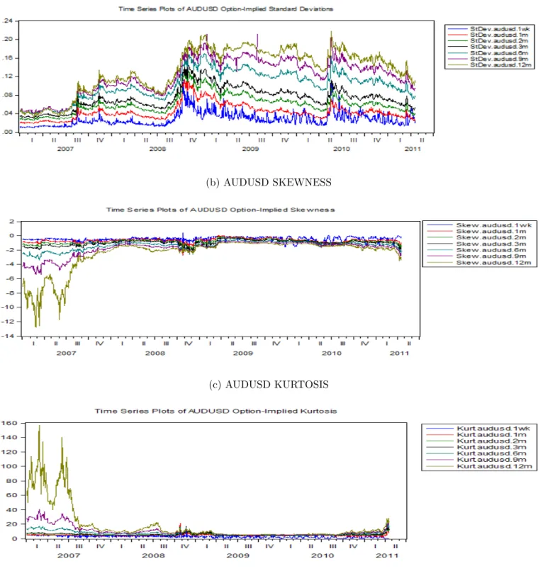
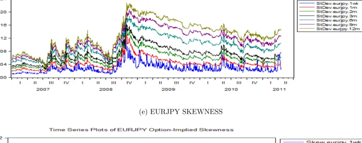
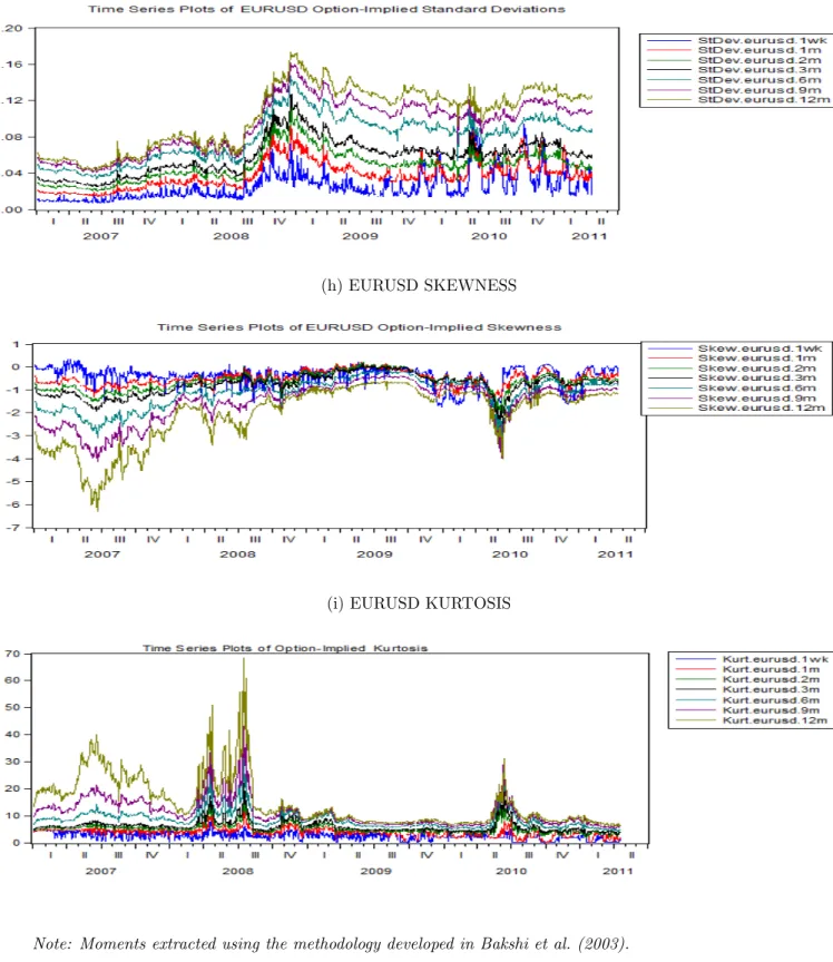
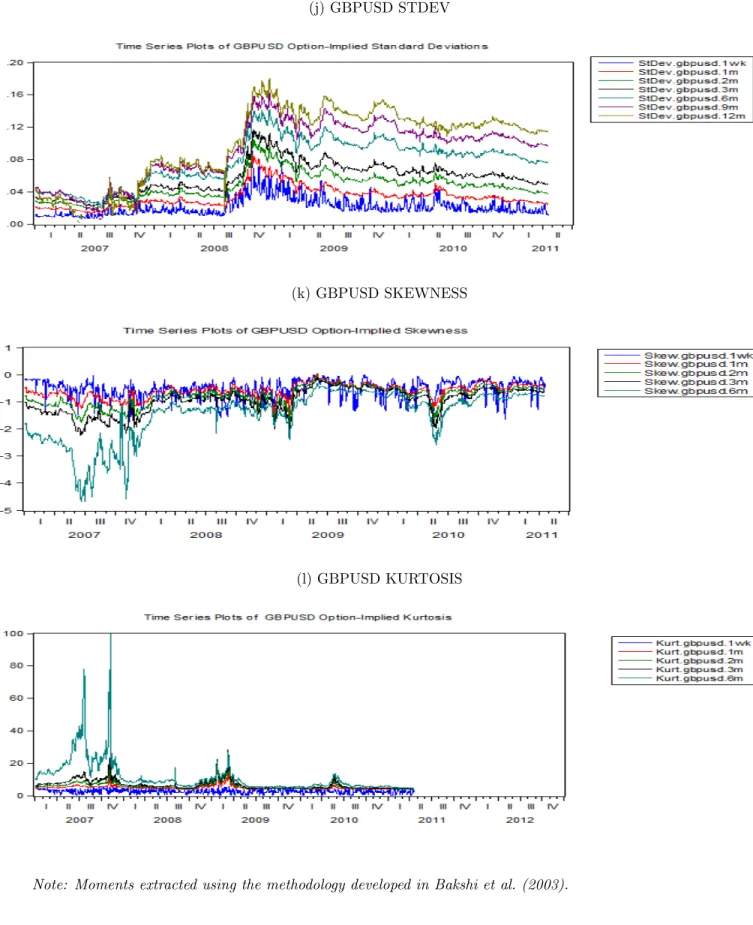
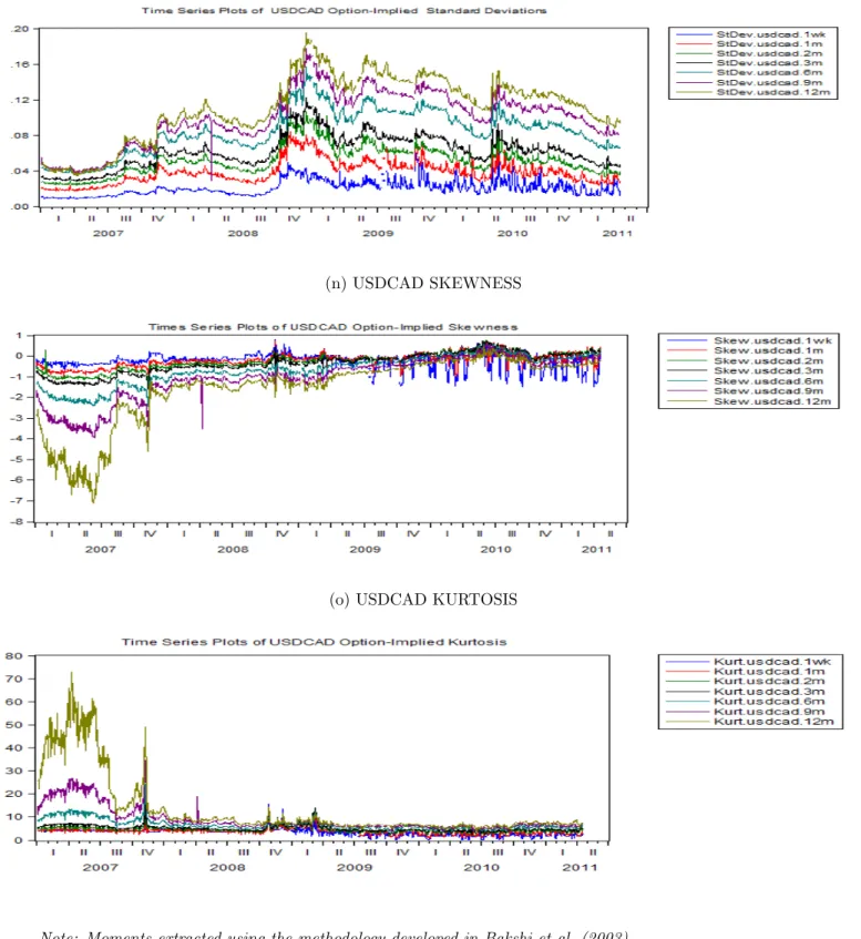
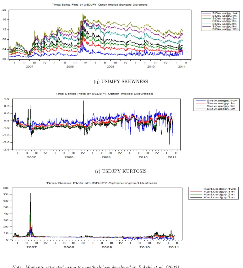
Time series plots of the extracted risk neutral moments of logST
St are shown in figure (2).
The extracted moments are very persistent, with AR(1) coefficients as high as 0.99. Zivot and Andrews (1992) unit root tests, however, suggest that almost all the implied moments are stationary,with structural breaks in the means on dates around late 2008 and early 2009. There are also some outliers in some of the skewness and kurtosis series, especially for 9m
and 12m tenor.31
INSERT FIGURE (2) HERE
4.2
Can the term structure of implied moments predict currency
returns?
For each currency pair i, we start by estimating the standard UIP regression
sit+τ −sit=α+β(ftt+τi−sit) +it+τ. (4.1)
We focus on model fit and joint significance rather than testing whether the β coefficient
is equal to 1. Fitted vs Actual plots of estimated regression (4.1) (with breaks) are shown
in figures 4(a)-4(e), while condensed results can be found in column A of table (3). For all
currency pairs, the forward premia coefficients are statistically significant at the 1% level,
and adjusted R2 of at least 10% for each currency pair.
We then consider the predictive ability of τ-period option-implied higher moments by
estimating the following augmented UIP regression:
sit+τ −sit =α+β1(fti,t+τ −st) +β2stdev i,t+τ t +β3skew i,t+τ t +β4kurt i,t+τ t +i,t+τ (4.2)
Equation (4.2) therefore augments the standard UIP equation (4.1) by studying the predictive ability of the 1st−4th moments of the distribution of logSt+τ
St
. The condensed regressions
results are shown in column B table (3) . The adjusted R2s for the matched-frequency
augmented UIP regressions are consistently higher than those from the standard UIP specification
in columnA, ranging from 26% to 67%. Coefficients on the higher order moments are always
jointly significant at the 1% level.
We next estimate a term structure modification of the standard UIP equation (4.1) that uses information contained in the term structure of forward premia to predict exchange rate movements: sit+τ −sit =γ0,τ + 3 X j=1 γ1,jP CjmeanT erm+it+τ. (4.3)
Condensed results from regression specification (4.3) are presented in column Cof table (3).
Comparing columns A and C in table (3), we see that adding the whole term structure of
forward premia significantly improves the UIP regression fit. For example, the adjusted R2
jumps from 27% to 57% for AUDUSD, 15% to 40% for EURUSD and from 15% to 54% for USDCAD.
Lastly, we regress exchange rate movements on the term structure of 1st−4th moments:
sit+3M −sit=γ0,τ + 3 X j=1 γ1,jP CjmeanT ermi+ 3 X j=1 γ2,jP CjstdevT ermi+ 3 X j=1 γ3,jP CjskewT ermi+ 3 X j=1 γ4,jP CjkurtT ermi+it+3M. (4.4)
Plots of actual versus fitted values from regressions (4.4) and (4.1) are shown in figures (4). These plots show that considered with the standard UIP regression, accounting for higher order moment risks and expectations substantially improves that model fit. The condensed regression results for the higher moment term structure specification, shown in
columnDof table (3) show that compared to the UIP specification in columnA, accounting
of for higher moments and expectations,for example, increases adjustedR2 from 27% to 67%
for AUDUSD, 15% TO 53% for EURUSD and from 10% to 57% for USDJPY.
4.3
Can option-implied moments forecast FX excess returns?
4.3.1 Matched Frequency Analysis: Predictive ability of the volatility smile
For each currency pair i, we start by investigating the predictive ability of τ − period
option-implied measures of standard deviation, skewness and kurtosis for subsequent excess currency returns32: fti,t+τ−Et(sti+τ) =γ0,τ +γ1,τstdev i,t+τ t +γ2,τskew i,t+τ t +γ3,τkurt i,t+τ t +ui,t+τ. (4.5)
Under rational expressions,fti,t+τ−Et(sit+τ) is also equal to the risk premium. Gereben (2002)
and Malz (1997) also estimate regression specification (4.5) and interpret the results in light of the time-varying risk premia explanation of the UIP puzzle. Gereben (2002) argues that if the forward bias is due to time-varying risk premia, then variables that capture the nature of FX risk should be able to explain the dynamics of the forward bias. The option-implied moments on the RHS in regression equation 4.5), which capture perceived FX volatility, tail and crash risk should therefore be able to explain the forward bias. Malz (1997) also argues that statistical significance of the coefficient on skewtt+τ can be interpreted as providing support for the peso problem explanation of the UIP puzzle.
Going back to expression 4.5), we note thatEt(st+τ) is not observable. If we assume that
market participants have rational expectations, then Et(st+τ) and st+τ will only differ by a
forecast errorνt+1 that is uncorrelated with all variables that use information at timet, such that
st+τ =Et(st+τ) +νt+1. (4.6)
Plugging equation (4.6) into equation (4.5) and rearranging gives us the following estimable
32Excess returns are a component of the expected exchange rate movements since
Et(sit+τ)−s i
t can be
regression equation: xrt+τ =γ0,τ +γ1,τstdev t+τ t +γ2,τskew t+τ t +γ3,τkurt t+τ t +t+τ (4.7)
where the error term t+τ = ut+τ + νt+τ and xrt+τ is ex-post excess returns defined in
expression (2.3).
To provide intuition regarding expected coefficient signs in the regression equation (4.7), we take the point view of a domestic investor who invests in domestic bonds using money borrowed from abroad. As shown in equation (2.3), such an investor benefits from higher domestic interest rates as well as appreciation of domestic currency. Let’s also assume that the home currency is riskier, such that our investor would demand higher excess returns for
higher stdev and kurtosis in the exchange rate. If investors are averse to high variance and
kurtosis, they would require higher excess returns for holding bonds denominated in units
of the riskier domestic and we would expect the coefficients on stdev and kurtosis to be
both positive. We expect the skew coefficient to be positive for investor’s with preference
for positive skewness. Such an investor will require higher compensation for an increase in
skew, which represents a higher perceived likelihood of domestic currency depreciation.
Given the discussion in subsection (2.2.2), however, we note that pinning down the coefficient signs a priori is impossible without making further assumptions about the investor’s utility function or orthogonality of the moments. In our regression analysis, we therefore focus mainly on joint significance of the explanatory variables and model fit rather than on significance and signs of individual coefficients.
Sub-sample analyses suggest the presence of structural breaks in the matched-frequency regression relationships for the majority of currency pairs and tenors. We use the Bai and
Perron (2003) structural break test to identify the date for the most prominent break33 and
33We only focus on the major breaks, and therefore do not choose the number of breaks according to
estimate a modification of regression equation (4.7) that includes interactions with structural break indicator variable:
xrit+τ =γ0,τ +γ00,τD1i,τ +D1i,τ ∗γ1,τstdevi,tt +τ+D1i,τ ∗γ2,τskewi,tt +τ+D1i,τ∗
γ3,τkurti,tt +τ +γ4,τstdevti,t+τ +γ5,τskewti,t+τ +γ6,τkurtti,t+τ +it+τ.
(4.8)
where D1i,τ is an indicator variable that is zero before the break date and equal to one
otherwise.
The matched-frequency results, shown in tables 5(a)-5(f), demonstrate a consistent ability of options-based measures of FX standard deviation, skewness and kurtosis-proxying to explain excess currency returns. The coefficients on the six non-intercept terms are always
jointly significant at the 1% level. The adjustedR2sfor example, range from 13% (USDJPY)
to 28% for 1 month tenor and from 20%(USDJPY) to 42% (EURJPY) for the 3M tenor. We next go beyond OLS regression, which models the conditional mean of the the dependent variable given the explanatory variables, by using quantile regression analysis (QR) to investigate the predictive ability of options-based FX risk measures for the entire distribution of ex-post excess currency returns. By modeling the entire distribution of the dependent variable, QR allows us to get a more complete picture of the predictive ability of the option-implied moments. QR also has a further advantage over OLS in that it is robust to outliers in the dependent variable and does not impose restrictive distributional assumptions on the error terms.
We estimate the following linear quantile regression model, modified to include one break:
Qxri (θ|.) = γ0,τ +γ1,τST DEVti,t+τ +γ2,τSKEWti,t+τ +γ3,τKU RTti,t+τ +i,t+τ, (4.9)
where Qxri (θ|.) is the θth quantile of excess returns given information available at time t.34 Matched-frequency quantile regression results for 3M tenor are shown in tables
(7a)-(7f). We find that the coefficients on non-intercept terms are always jointly significant
across quantiles for all currency pairs. Adjusted R2s range from 13% to 44% for AUDUSD,
and 12% to 30% for USDJPY for example. Another consistent pattern across currency pairs and tenors is that option-implied moments have more predictive ability for lower and upper quantiles of excess returns than the middle quantiles.
INSERT TABLES (7a)- (7f)HERE
4.3.2 Can the term structure of implied moments predict excess currency returns?
We first extend regression equation (4.7) by regressing 3M bilateral excess returns on 1M,
3M and 12M option-implied moments. That is, for each currency pair i, we estimate the
following OLS regression:
xrti+3M =γ0,3M+X j γ1,τjstdevt+τj,i t + X j γ2,τjskewt+τj,i t + X j γ3,τjkurtt+τj,i t +it+3M, (4.10)
where j ∈ {1M,3M,12M}. Similar to the matched-frequency analysis in subsection (4.3.1),
our final term structure regression model is a modification of (4.10) in which we include interactions with a structural break indicator variableD1. Regression results from specification
(4.10) (with break ) are shown in columnBof table (2). Compared to the matched frequency
results presented in column A, we see a huge increase in the adjusted R2s. For example,
adjusted R2 increases from 33% to 62% for AUDUSD, 34% to 49% for EURUSD, and from
20% to 36% for USDJPY.
In column C of table (2) , we present condensed results of regressions that incorporate
information from all tenors (not just 1M,3M and 12M) by using principal components extracted from all tenors.
xrti+3M =γ0,τ + 3 X j=1 γ2,jP CjstdevT ermi+ 3 X j=1 γ3,jP CjskewT ermi+ 3 X j=1 γ4,jP CjkurtT ermi+it+3M. (4.11)
In equation (4.11), P CjxxxxT ermi refers to the jth principal component extract from
the currency i term structure of option-implied moment xxxx. Results from estimation
regression equation (4.11) are in column Cof table (2).
Lastly, we extend the specification in (4.11) by adding information from the term structure of first moments as additional regressors:
xrti+3M =γ0,τ + 3 X j=1 γ1,jP CjmeanT ermi+ 3 X j=1 γ2,jP CjstdevT ermi+ 3 X j=1 γ3,jP CjskewT ermi+ 3 X j=1 γ4,jP CjkurtT ermi+it+3M. (4.12)
The term structure of first moments captures expectations of the dynamics of future macroeconomic fundamentals. We use the term structure of interest rate differentials to
extract the principal components of the term structure of first moments of logSt+τ
St ) .
35
Using yield curve data to extract the term structure of first moments has the advantage of allowing us to also use interest rate differentials for tenors not covered by our option price data. As with our previous regressions, we estimate a version of regression model (4.12) that includes interactions with a structural break indicator variable.
The condensed results from estimating equation (4.12) with breaks are presented in
column (D) of table (2). Actual vs fitted plots from this regression are shown in figures
35As noted earlier,the forward premium, which is the theoretical mean of the risk-neutral probability
density of logSt+τ
S
(3(a)-3(e)).
INSERT FIGURE (3) AND TABLE (2) HERE
Compared to the matched frequency regressions columnAof table (2), inclusinf the term
structure of 1st −4th moments increases the adjusted R2 from 33% to 66% for AUDUSD,
34% TO 51% for EURUSD, 48% to 83% for GBPUSD, 48% to 62% for USDCAD and from 20% to 57% for USDJPY. These dramatic improvements in the model fit further highlight the importance of properly accounting for expectations and higher moment risks.
5
Conclusion
This paper has documented a robust ability of options-implied measures of FX higher moment risks to explain subsequent excess currency returns and FX returns. We also find that the term structure of such risks, capturing forward-looking property of the exchange rate, add further explanatory power. Our findings suggest that expectation and risk should be given more careful consideration in the structural modeling and empirical testing of exchange rate models.
This paper can be extended in several directions that are useful to academics,monetary policy officials and investment professionals. First, how useful is the option-based information for out-of-sample forecasting of exchange rate. The ability to accurately forecast exchange rates movements for many purposes, including determining the future value of foreign denominated debt payments and for hedging for investment managers exploiting international investment opportunities. Second, an empirical analysis of the macroeconomic variables and events that drive the option-implied moments would further shed light on the link between exchange rates and fundamentals. Lastly, it might be worthwhile to
References
Bacchetta, P. and E. van Wincoop (2009), “Predictability in financial markets:what do
survey data tell us?” Journal of International Money and Finance, 28, 406–426.
Bai, J. and P. Perron (2003), “Computation and analysis of multiple structural change
models.” Journal of Applied Econometrics, 18, 1–22.
Bakshi, G., N. Kapadia, and D. Madan (2003), “Stock return characteristics,skew laws, and the differential pricing of individual equity options.” Review of Finacial Studies, 6, 101–143.
Breeden, D. and R. Litzenberger (1978), “Prices of state contingent claims implicit in
options.” Journal of Business, 51, 621–652.
Burnside, C., M. Eichenbaum, I. Kleschchelski, and S. Rebelo (2011), “Do peso problems
explain the returns to the carry trade?” Review of Financial Studies, 24, 853–891.
Carr, P. and D. Madan (2001), “Optimal positioning in dervative securities.” Quantitative
Finance, 1, 19–37.
Castagna, A. (2010), FX Options and Smile Risk. WILEY, United Kingdom.
Castagna, Antonio and Fabio Mercurio (2005), “Consistent pricing of fx options.” SSRN
Working Paper No 873788.
Castagna, M. and F. Mercurio (2007), “The vanna-volga method for implied volatilities.”
Risk, 20, 106–111.
Chen, Y-c. and K-P. Tsang (2013), “What does the yield curve tell us about exchange rate
Clarida, R.H., L. Sarno, M.P Taylor, and G. Valente (2003), “The out-of-sample success of
term structure models as exchange rate predictors:a step beyond.”Journal of International
Economics, 60, 61–83.
Clarida, R.H. and M.P. Taylor (1997), “The term structure of forward exchange rate
premiums and the forecastability of spot exchange rates:correcting the errors.” Review
of Economics and Statistics, 79, 353–361.
Diebold, F.X., Piazzesi M., and Rudebusch G.D. (2005), “Modeling bond yields in finance
and macroeconomics.” American Economic Review, 95, 415–420.
Engel, C. (1996), “The forward discount anomaly and the risk premium: A survey of recent
evidence.”Journal of Empirical Finance, 3, 123–192.
Engel, C. and K. D. West (2005), “Exchange rates and fundamentals.” Journal of Political
Economy, 113, 485–517.
Engel, Charles (2013), “Exchange rates and interest parity.” In Handbook of International
Economics,vol. 4,Forthcoming (Gita Gopinath, Elhanan Helpman, and Kenneth Rogoff, eds.), Elsevier.
Eviews (2013), “Eviews 8 guide ii.”
Fama, E. and K. R. French (1993), “Common risk factors in the returns on stocks and
bonds.” Journal of Financial Economics, 33, 3–56.
Fama, Eugene F. (1984), “Forward and spot exchange rates.” Journal of Monetary
Economics, 14, 319–38.
Gereben, A. (2002), “Extracting market expectations from option prices:an application to
Grad, D. (2010), “Foreign exchange risk premia and macroeconomic announcements:evidence
from overnight currency options.”Unpublished Dissertation Chapter.
Hansen, L. P. and R.J. Hodrick (1980), “Forward rates as unbiased predictors of future spot
rates.”Journal of Political Economy, 99, 461–70.
Jondeau, Eric, Ser-Huang Poon, and Michael Rockinger (2010), Financial Modeling under
non-gaussian distributions. Springer, United States.
Jurek, J. (2009), “Crash-neutral currency carry trades.” Princeton University Working
Paper.
Koenker, Roger and Jose Machado (1999), “Goodness of fit and related inference processes
for quantile regression.” Journal of the American Statistical Association, 94, 1296–310.
Lustig, H., N. Roussanov, and A. Verdelhan (2011), “Common risk factors in currency
markets.” Review of Financial Studies, 24, 3731–3777.
Malz, A. (1998), “Option prices and the probability distribution of exchange rates.” In
Currency Options and Exchange Rate Economics (Zhaohui Chen, ed.), 108–137, World Scientific.
Malz, A.M. (1997), “Option-implied probability distributions and currency excess returns.”
Federal Reserve Bank of New York Staff Report, 32.
Mark, N. (1995), “Exchange rates and fundamentals:evidence on long-horizon predictability.”
American Economic Review, 85, 201–218.
Mark, N. C. (2001), International Macroeconomics and Finance. Blackwell Publishing,
United States.
Renaud, Olivier and Maria-Pia Victoria-Fraser (2010), “A robust coefficient of determination for regression.”Journal of Statistical Planning and Inference, 142, 1852–1862.
Scott, R.C. and P.A. Horvath (1980), “On the direction of preference for moments of higher
order than the variance.”Journal of Finance, 35, 915–919.
Verdelhan, A. (2012), “The share of systematic variation in bilateral rates.”Working Paper.
Zivot, E. and D. W. K. Andrews (1992), “Further evidence on the great crash,the oil price
shock and the unit root hypothesis.” Journal of Business and Economic Statistics, 10,
Figure 1: Profit diagrams for options strategies
(a) Profit Function of a Straddle (b) Profit Function of a Risk Reversal
(c) Profit Function of a Strangle (d) Profit Function of a Butterfly
Figure 2: Time Series Evolution Of Option Implied Moments (a) AUDUSD STDEV
(b) AUDUSD SKEWNESS
Figure 2: Time Series Evolution Of Option Implied Moments (d) EURJPY STDEV
(e) EURJPY SKEWNESS
(f) EURJPY KURTOSIS
Figure 2: Time Series Evolution Of Option Implied Moments (g) EURUSD STDEV
(h) EURUSD SKEWNESS
(i) EURUSD KURTOSIS
Figure 2: Time Series Evolution Of Option Implied Moments (j) GBPUSD STDEV
(k) GBPUSD SKEWNESS
(l) GBPUSD KURTOSIS
Figure 2: Time Series Evolution Of Option Implied Moments (m) USDCAD STDEV
(n) USDCAD SKEWNESS
(o) USDCAD KURTOSIS
Figure 2: Time Series Evolution Of Option Implied Moments (p) USDJPY STDEV
(q) USDJPY SKEWNESS
(r) USDJPY KURTOSIS
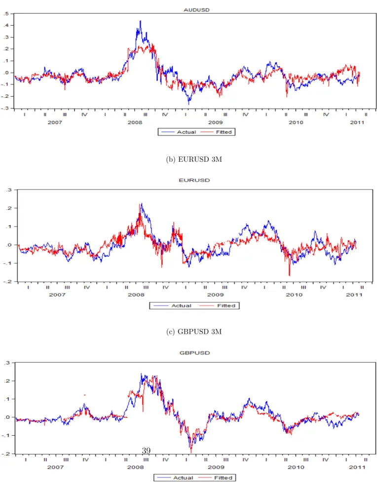
Figure 3: Quarterly FX Excess Returns on Term Structure of 1st to 4th Moments+Break
(a) AUDUSD 3M
(b) EURUSD 3M
(c) GBPUSD 3M
Note: Fitted vs Actual plots from the regression of 3M excess return, as defined in expression (2.3), on 39
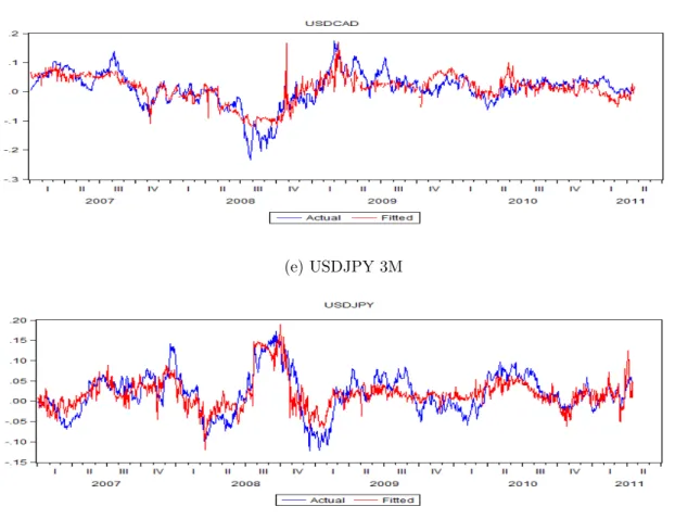
Figure 3: Quarterly FX Excess Returns on Term Structure of 1st to 4th Moments+Break (d) USDCAD 3M
(e) USDJPY 3M
Note: Fitted vs Actual plots from the regression of 3M excess return, as defined in expression (2.3), on the first three principal components from the term structure of extracted moments ofπQt lnST
St
(Regression specification in expression (4.12). Condensed regression results are in column D of table (2) .
Figure 4: Quarterly FX Movements on Term Structure of 1st to 4th Moments+Break
(a) AUDUSD 3M RET
(b) EURUSD 3M RET
(c) GBPUSD 3M RET
Fitted vs Actual plots from the regression of 3M logST
St
on the first three principal components from the 41
Figure 4: Quarterly FX Movements on Term Structure of 1st to 4th Moments+Break
(d) USDCAD 3M RET
(e) USDJPY 3M RET
Fitted vs Actual plots from the regression of 3M logST
St
on the first three principal components from the term structure of extracted moments ofπQt lnST
St
(Regression specification in expression (4.4). Condensed regression results are in column D of table (3) .
Figure 5: Quarterly FX Movements on Term Structure of Global Risk+Break (a) AUDUSD 3M RET
(b) EURUSD 3M RET
(c) GBPUSD 3M RET
Fitted vs Actual plots from the regression of 3M logST
St
Figure 5: Quarterly FX Movements on Term Structure of 1st to 4th Moments+Break (d) USDCAD 3M RET
(e) USDJPY 3M RET
Fitted vs Actual plots from the regression of 3M logST
St
on the first three principal components from the term structure of extracted moments ofπQt lnST
St
(Regression specification in expression (4.4). Condensed regression results are in column D of table (3) .
T able 1: O-T-C Mark et Statistics and Con v en tions A. Quoting Con v en tions in o v er-the-coun ter FX Options Mark et Sym b ol Definition Base currency Domestic currency P ositiv e Sk ew means A UDUSD USD p er A UD A UD US D US D depreciation EURJPY JPY p er EUR EUR J PY EUR depr e ciation EUR USD USD p er EUR EUR US D US D depreciation GBPUSD USD p er GBP GBP USD USD depreciation USDCAD CAD p er USD USD CAD CAD depreciation USDJPY JPY p er USD USD JPY JPY depreciation B. Sample Ann ualized Implied V olatilities T enor A TM 25D RR 25D VWB 10D RR 10D VWB 1 W eek 7.352 -0.495 0.131 -0.847 0.379 1 Mon th 6.851 -0.347 0.136 -0.584 0.389 2 Mon th 6.851 -0.366 0.157 -0.619 0.449 3 Mon th 6.851 -0.396 0.162 -0.663 0.485 6 Mon th 6.901 -0.426 0.187 -0.703 0.54 9 Mon th 7.051 -0.446 0.197 -0.743 0.571 12 Mon th 6.901 -0.426 0.187 -0.703 0.54 C. Av era ge Daily T urno v er in FX mark et (billions) 1998 2001 2004 2007 2010 2013 Sp ot FX T ransactions 568 386 631 1005 1488 2046 P ercen tage Change N/A -32 63.5 59.3 48.3 37.5 FX Deriv ativ es Outrigh t F orw ards 128 130 209 362 475 680 FX Sw aps 734 656 954 1714 1759 2228 Options and other pro ducts 87 60 119 212 207 337 P ercen tage Change N/A -31 98.3 83 -2.4 62.8 Exc hange T raded De riv ativ es 11 12 26 80 155 160 Note: “A TM” is at-the-money str add le, 25D RR and 10D RR ar e 25%-and 10%-delta risk reversals resp ectively; and 25D VWB and 10D VWB ar e 25%-and 10%-delta V ega-weighte d butterflies resp ectively. Se e Se ction (3.3) for mor e details. The numb ers in table (1C) ar e fr om Bank of International Settlements (2013). In table (1C) , “ other pr o ducts” refers to “highly lever ege d tr ansactions and/or tr ades whose notional amount is variable and wher e a de comp osition into individual plain vanil la comp onents was impr act ic al or imp ossible” Bank of International Settlem ent s (2013).
Table 2: Higher Moment & Term Structure Predictors of Quarterly FX Excess Returns A B C D AUDUSD # of observations 1122 1120 1106 1039 Adjusted R2 0.33 0.6243 0.5693 0.6621 P(F-stat) 0.00 [0.00,0.00,0.00] [0.00,0.00,0.00] [0.00,0.00,0.00,0.00] Break Date 1/29/2009 6/30/2008 5/12/2008 5/30/2008 EURUSD # of observations 1117 1105 1093 1093 Adjusted R2 0.34 0.4895 0.4704 0.5104 P(F-stat) 0.00 [0.00,0.00,0.00] [0.00,0.00,0.00] [0.00,0.00,0.00,0.00] Break Date 2/4/2009 1/29/2009 1/29/2009 2/2/2009 GBPUSD # of observations 1121 1055 1050 980 Adjusted R2 0.48 0.7217 0.653 0.8334 P(F-stat) 0.00 [0.00,0.00,0.00] [0.00,0.00,0.00] [0.00,0.00,0.00,0.00] Break Date 10/24/2008 10/24/2008 10/24/2008 5/27/2008 USDCAD # of observations 1116 1095 1092 1016 Adjusted R2 0.48 0.5968 0.5824 0.6151 P(F-stat) 0.00 [0.00,0.00,0.00] [0.00,0.00,0.00] [0.00,0.00,0.00,0.00] Break Date 2/5/2009 5/5/2008 5/5/2008 5/2/2008 USDJPY # of observations 1121 1107 1099 1099 Adjusted R2 0.2 0.3605 0.3673 0.5668 P(F-stat) 0.00 [0.00,0.00,0.00] [0.00,0.00,0.00] [0.00,0.00,0.01,0.00] Break Date 7/4/2008 7/22/2008 7/21/2008 7/22/2008
Note: In all equations, dependent variable is quarterly excess currency returns, as defined in
equation (2.3). All regressions are estimated with interactions with a break indicator variable D1.
Breakdate for each equation found using Bai and Perron (2003) method. Column A is from the
matched-frequency regression in equation (4.7): Column B is regression from columnA but with
1M and 12M stdev, skew and kurt added as additional regressors ( see equation 4.10 ). Three P values are for Wald tests for the null that coefficients on each group of moments [stdev,skew,kurt]
are all zero. In column C we use the first three principal components extracted from each of
stdev,skew and kurt for all tenors( equation 4.11). Column D is regression from columnC but
with the first three principal components from relative yields (proxying for first moment for the
term stucture of first moments) added as additional regressors. In column D (equation 4.12), P
Table 3: Higher Moment and Term Structure Predictors of Quarterly FX Returns A B C D AUDUSD # of observations 1122 1122 1054 1039 Adjusted R2 0.2656 0.3457 0.564 0.6704 P(F-stat) 0.00 0.00 0.00 [0.00,0.00,0.00,0.00] Break Date 10/6/2008 1/29/2009 1/13/2009 5/30/2008 EURUSD # of observations 1117 1117 1093 1093 Adjusted R2 0.148 0.366 0.3996 0.5302 P(F-stat) 0.00 0.00 0.00 [0.00,0.00,0.00,0.00] Break Date 3/10/2008 2/4/2009 5/16/2008 2/2/2008 GBPUSD # of observations 1116 1121 1045 980 Adjusted R2 0.5254 0.6682 0.6349 0.839 P(F-stat) 0.00 0.00 0.00 [0.00,0.00,0.00,0.00] Break Date 7/1/2008 6/30/2008 7/7/2008 5/27/2008 USDCAD # of observations 1121 1116 1037 1016 Adjusted R2 0.1561 0.493 0.5359 0.6234 P(F-stat) 0.00 0.00 0.00 [0.00,0.00,0.00,0.00] Break Date 9/11/2007 2/5/2009 10/15/2008 5/2/2008 USDJPY # of observations 1121 1121 1112 1099 Adjusted R2 0.1033 0.2619 0.2846 0.5774 P(F-stat) 0.00 0.00 0.00 [0.00,0.00,0.01,0.00] Break Date 7/4/2008 7/4/2008 7/4/2008 7/22/2008
Note: In all equations, dependent variable is quarterly currency returns,ln
St+3M
St
. All
regressions are estimated with interactions with a break indicator variable D1. Breakdate for each
equation found using Bai and Perron (2003) method. Column A is from the standard UIP
regression ( equation (4.1)) : sit+τ−sit=α0+α1∗D1i,τ +β1(f t+τ ,i t −sit) +β2D1i,τ ∗(f t+τ ,i t −sit) +it+τ
P values in column A are for the null hypothesis thatβ1 =β2 = 0 . Column B is column A with
quarterly stdev, skew and kurt also added(equation (4.2,with break) In Column C(equation (4.3 )
) , we extract the first 3 Principal components from relative yields and use them as regressors
(term structure of first moments as regressors). In column D ( equation 4.4) we extract principal
components from each of stdev,skew, kurtosis, and use them as additional regressors from the
Table 4: Global Risk XR Regressions
A B C D
Matched Frequency XR Term Structure XR Matched Frequency RET Term Structure RET
AUDUSD # of obs. 1109 976 1109 976 Adj. R2 0.614 0.632 0.622 0.64 P(F-stat) 0 0 0 0 Break date 5/9/2008 10/6/2008 5/9/2008 10/6/2008 EURUSD # of obs. 1109 976 1109 976 Adj. R2 0.452 0.486 0.255 0.495 P(F-stat) 0 0 0 0 Break date 4/16/2010 5/3/2010 10/22/2009 5/3/2010 GBPUSD # of obs. 1109 976 1109 976 Adj. R2 0.591 0.664 0.602 0.674 P(F-stat) 0 0 0 0 Break date 10/24/2008 12/17/2008 10/24/2008 12/17/2008 USDCAD # of obs. 1109 976 1109 976 Adj. R2 0.651 0.638 0.656 0.64 P(F-stat) 0 0 0 0 Break date 7/4/2008 1/30/2009 7/4/2008 1/30/2009 USDJPY # of obs. 1109 976 1109 976 Adj. R2 0.552 0.572 0.556 0.573 P(F-stat) 0 0 0 0 Break date 7/4/2008 7/4/2008 7/4/2008 7/4/2008
Note: In column A, for each quarterly excess return, we use the first three principal
components extracted from the 3-month risk-neutral moments of all currencies as regressors. In column B, For each quarterly excess return, we use the first three principal components extracted from each moments for all tenors and all currencies as regressors. In column C, for each quarterly exchange rate change, we use the first three principal components
extracted from the 3-month risk-neutral moments of all currencies as regressors. In column D, for each quarterly exchange rate change , we use the first three principal components extracted from each moments for all tenors and all currencies as regressors. Newey-West standard deviations are reported in brackets, with asterisks indicating significance at 1%