San Jose State University
SJSU ScholarWorks
Master's Projects Master's Theses and Graduate Research
Fall 2015
SSCT Score for Malware Detection
Srividhya Srinivasan
San Jose State University
Follow this and additional works at:https://scholarworks.sjsu.edu/etd_projects Part of theComputer Sciences Commons
This Master's Project is brought to you for free and open access by the Master's Theses and Graduate Research at SJSU ScholarWorks. It has been accepted for inclusion in Master's Projects by an authorized administrator of SJSU ScholarWorks. For more information, please contact Recommended Citation
Srinivasan, Srividhya, "SSCT Score for Malware Detection" (2015).Master's Projects. 444. DOI: https://doi.org/10.31979/etd.4brm-b25z
SSCT Score for Malware Detection
A Project Presented to
The Faculty of the Department of Computer Science San Jose State University
In Partial Fulfillment
of the Requirements for the Degree Master of Science
by
Srividhya Srinivasan December 2015
c
○2015
Srividhya Srinivasan ALL RIGHTS RESERVED
The Designated Project Committee Approves the Project Titled SSCT Score for Malware Detection
by
Srividhya Srinivasan
APPROVED FOR THE DEPARTMENTS OF COMPUTER SCIENCE SAN JOSE STATE UNIVERSITY
December 2015
Dr. Mark Stamp Department of Computer Science Dr. Thomas Austin Department of Computer Science Dr. Christopher Pollett Department of Computer Science
ABSTRACT
SSCT Score for Malware Detection by Srividhya Srinivasan
Metamorphic malware transforms its internal structure when it propagates, mak-ing detection of such malware a challengmak-ing research problem. Previous research con-sidered a score based on simple substitution cryptanalysis, which was applied to the metamorphic detection problem. In this research, we analyze a new score based on a combined simple substitution and column transposition (SSCT) cryptanalysis. We show that this SSCT score significantly outperforms the simple substitution score— and other malware detection scores—in many cases.
ACKNOWLEDGMENTS
I would like to thank my project advisor Dr. Mark Stamp for all his guidance and mentoring during the course of this project. I would also like to thank my committee members Dr. Thomas Austin and Dr. Christopher Pollett for reviewing my work and providing valuable feedback.
TABLE OF CONTENTS CHAPTER
1 Introduction . . . 1
2 Previous Work . . . 4
2.1 Jakobsen’s Algorithm . . . 4
2.2 Simple Substitution Distance . . . 5
3 Simple Substitution Columnar Transposition . . . 8
3.1 SSCT Encryption . . . 8
3.2 Attack on SSCT Using Jakobsen’s Algorithm . . . 9
3.3 SSCT for Malware Detection . . . 11
4 Experiments and Results . . . 14
4.1 Dataset . . . 14
4.2 Parameters . . . 16
4.3 Results . . . 17
5 Conclusion and Future Work . . . 22
APPENDIX Experiments . . . 26
LIST OF TABLES
1 Caesar Cipher with key = 2 . . . 5
2 Expected digraph frequency E . . . 7
3 Putative key . . . 7 4 Digraph frequency D . . . 7 5 Digraph frequency D . . . 7 6 Substitution Key . . . 8 7 Intermediate matrix . . . 9 8 Ciphertext matrix . . . 9
9 Final ciphertext matrix . . . 9
10 Initial ciphertext matrix . . . 10
11 Compute 𝐸 Matrix . . . 11
12 Compute Score . . . 12
13 Jakobsen’s Algorithm . . . 13
14 Dataset . . . 15
LIST OF FIGURES
1 Scatter Plot NGVCK . . . 18
2 NGVCK ROC Curve . . . 19
3 Scatter Plot Cridex . . . 19
4 Cridex ROC Curve . . . 20
A.5 Scatter Plot MWOR 0.5 . . . 26
A.6 Scatter Plot MWOR 1 . . . 27
A.7 Scatter Plot MWOR 1.5 . . . 27
A.8 Scatter Plot MWOR 4 . . . 28
A.9 Scatter Plot SecurityShield . . . 28
A.10 Scatter Plot ZBOT . . . 29
A.11 Scatter Plot SmartHDD . . . 29
A.12 Scatter Plot Harebot . . . 30
A.13 Scatter Plot Winwebsec . . . 30
A.14 MWOR0.5 ROC Curve . . . 31
A.15 MWOR1 ROC Curve . . . 31
A.16 MWOR1.5 ROC Curve . . . 32
A.17 MWOR4 ROC Curve . . . 32
A.18 SecurityShield ROC Curve . . . 33
A.19 ZBOT ROC Curve . . . 33
A.20 SmartHDD ROC Curve . . . 34
A.22 Winwebsec ROC Curve . . . 35 A.23 Scatter Plot Winwebsec IC Scores . . . 35 A.24 Winwebsec ROC Curve(IC Scores) . . . 36
CHAPTER 1 Introduction
Malware is a piece of software written with malicious intent. Over the years, malware have evolved to be more like benign software and hence it has become in-creasingly difficult to tell them apart from a normal harmless program [19]. The techniques used to detect malware files can be broadly classified under two categories - dynamic and static malware analysis. In dynamic analysis, the malware is allowed to be live in an emulated environment and its actions are observed. In static analysis, the information extracted from the malware file is used to analyze and decide whether the file is a malware or a benign file. Even from this high level definition, we can see that dynamic analysis techniques are, in most cases, more expensive in terms of running times than their static analysis counterparts.
Many malware detection techniques have been proposed and analyzed in the lit-erature. Examples of such malware detection techniques include the Hidden Markov Model approach in [1, 2], as well as a score that relies on simple substitution crypt-analysis [8]. The Simple Substitution Distance (SSD) malware score in [8] is based on Jakobsen’s algorithm [6], which is an extremely efficient attack on simple substitution ciphers. Consequently, the SSD score computation is fast and efficient, and in [8] it is shown to be very effective against some challenging classes of malware.
Signature-based virus detection systems search for a known pattern of bits or a signature in the body of the malware. If malwares had stopped evolving, all viruses could be detected by these systems. Unfortunately, that is not the case. Malware developers constantly look for techniques to break the performance of the virus
de-tection systems and sadly, keep succeeding in their attempts. Morphing the malware code is one such technique used to evade signature detections.
Polymorphic malware consists of the malware code, which is encrypted, and a module containing the decryption logic [13]. The decryption module is also morphed so that it does not adopt a common signature. Metamorphic virus follows a similar principle and mutates the virus body before infecting a system. There are several techniques available to achieve this including, but not limited to register renaming, renaming of subroutines and dead code insertion [13].
In both polymorphic and metamorphic viruses, each version of malware is differ-ent from the previous known version. Due to this, they are difficult to detect using the conventional signature based security systems. It is interesting to note that, through the evolution of different versions of these malware, the underlying functionality re-mains more or less the same. In such cases, it seems logical to view the known version of a malware as the “plaintext” and the newer, unknown version to be an encrypted cipher text. The unknown file or the ciphertext can be decrypted to see if it yields any of the known malware. If it cannot be decrypted successfully, we can assume that the unknown file is benign.
In this paper, we will discuss the use of an encryption technique called Simple Substitution Columnar Transposition as a way to distinguish a malware file from a benign file and compare the results obtained by this method with the existing techniques in static analysis. This paper is organized into the following sections. In this chapter, we have given a brief summary about polymorphic and metamorphic malware and how encryption techniques can be used as malware detection techniques. Chapter 2 talks about some existing implementation of this idea. In Chapter 3, we have an overview of the SSCT cryptanalysis technique followed by a detailed account
of our implementation. In Chapter 4, we present our experiments and the results obtained. We conclude with Chapter 5, which talks about the future work in this area.
CHAPTER 2 Previous Work
In this chapter, we will see some of the existing research that form the basis of our SSCT implementation. Since SSCT encryption is an extension of the Simple Sub-stitution technique, a deeper understanding of both the simple subSub-stitution method and the Jakobsen’s algorithm which helps in solving it, will help us in breaking the SSCT cipher.
2.1 Jakobsen’s Algorithm
The naive approach to decrypt a simple substitution cipher is outlined below: 1. Guess an initial key 𝐾
2. Decrypt the cipher using 𝐾
3. If the decrypted message does not make sense, modify the key 𝐾
4. Go to step 2
Jakobsen’s algorithm [6] provides a faster attack on the simple substitution cipher. This method makes use of digraph statistics of the plaintext and the ciphertext. Initially, the digraph frequencies of the plaintext letters are populated in the matrix
𝐸 and the digraph frequencies for the ciphertext are filled in the matrix 𝐷. We
compute the score for the initial 𝐷 matrix using the formula
Table 1: Caesar Cipher with key = 2
A B C D E F G H I J K L . . . S T U V W X Y Z C D E F G H I J K L M N . . . U V W X Y Z A B
An initial key 𝐾 is guessed by comparing the individual letter frequencies in the
plaintext and the ciphertext [4]. For every change in 𝐾, the 𝐷 matrix changes as
follows: if 𝐾𝑖 and 𝐾𝑗 are swapped, then we swap the 𝑖𝑡ℎ and 𝑗𝑡ℎ columns and rows in the 𝐷 matrix. We compute the score for the modified 𝐷 matrix. If the score
improves, we retain the changes, otherwise we swap the rows and columns again and continue with a different key.
2.2 Simple Substitution Distance
One of the earliest forms of encryption is the Caesar Cipher [13]. Here, the key is an integer indicating the shift in the alphabet position. For example, if the key is 2, every character in the alphabet maps to the character two units away from itself, as shown in Table 1. Simple Substitution is a modification of the Caesar Cipher where instead of a constant displacement, the key can be any permutation of the characters in the alphabet.
In static analysis, opcode sequences are often extracted from a known malware and compared to the opcode sequence from an unknown file [16]. By obtaining a similarity measure between the two sequences, the unknown file is classified either as a malware or a benign file. In these methods, opcodes are usually represented by characters from the English alphabet, making the extracted opcode sequence a string of letters from the English alphabet. Combining this representation and the opcode substitution that we saw in Chapter 1 to morph the malware, we can look at an unknown file as a cipher and try to decrypt it using the Simple Substitution method
to see if resembles any known version of the virus.
An effective implementation of the Simple Substitution method to detect malware is given in [8]. This implementation uses the Jakobsen’s algorithm to avoid repeated decryption of the cipher or the unknown file.
Let us try to simulate the Jakobsen’s algorithm on an example. Let us consider an alphabet with characters J,G,S,V and P in the decreasing order of their occurrence. Let the original digraph frequency in this alphabet be the matrix shown in Table 2. If our ciphertext is “GPSSPVJPSPSVJGSPJVJGSVSPVS”, based on the frequency, we can come with the putative key shown in Table 3. The decrypted text using this putative key is “PGJJGSVGJGJSVPJGVSVPJSJGSJ”. From this, we calculate the digraph frequencies and arrive at the matrix 𝐷 given in Table 4. We calculate the
score for this putative key using these two matrices 𝐸 and 𝐷. As per Jakobsen’s
algorithm, the next step is two modify this putative key 𝐾 and recompute the score.
There are several ways to modify the key, but to maintain the simplicity of this ex-ample, we swap the first two elements. When we decrypt now, the text obtained is “PJGGJSVJGJGSVPGJVSVPGSGJSG”. With this plaintext, the new digraph fre-quency matrix is given in Table 5. When we compare this with Table 4, we see that columns 1 and 2 and rows 1 and 2 are swapped. This means that we do not have to decrypt the ciphertext during every iteration in order to compute the score. Instead we can build the𝐷matrix once, and swap its rows and columns based on the changes
Table 2: Expected digraph frequency E J G S V P J 2 3 0 4 1 G 1 0 2 1 2 S 1 2 1 0 0 V 1 0 0 1 1 P 1 2 0 1 0
Table 3: Putative key S P V J G J G S V P
Table 4: Digraph frequency D J G S V P J 1 4 2 0 0 G 3 0 2 1 0 S 2 0 0 3 0 V 0 1 1 0 2 P 2 1 0 0 0
Table 5: Digraph frequency D J G S V P J 0 3 2 1 0 G 4 1 2 0 0 S 0 2 0 3 0 V 1 0 1 0 2 P 1 2 0 0 0
CHAPTER 3
Simple Substitution Columnar Transposition
We will first see how a piece of plaintext is encrypted using the simple substi-tution columnar transposition method. Once we have a clear understanding of the encryption, we can work backwards and come up with the steps to retrieve the plain-text from the cipherplain-text. This is crucial in implementing the scoring technique used in our project.
3.1 SSCT Encryption
Simple Substitution Columnar Transposition is a form of encryption that adds one more level of complexity to the simple substitution method. In this method, after the plaintext symbols are replaced with the ciphertext symbols, the text is written in the form of a matrix. The columns of this matrix are shuffled and the resulting text forms the ciphertext.
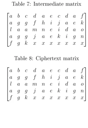
Let us encrypt the text “either the well was very deep or she fell very slowly” using SSCT, using the substitution key shown in Table 6. After substitution, the text now becomes “abcdaecdafaggfhijaeklaamneidaoaggjaekignfgk”. We fill this in-termediate ciphertext in a matrix as shown in Table 7. If the transposition key is (1,4,5,2,10,8,9,7,6,3), we get the final matrix as shown in Table 9. We obtain the ciphertext from this matrix, which in our case is
“adabfdacecafhgkaejiglmnaodaieaa-Table 6: Substitution Key
e i t h r w l a s v y d p o f a b c d e f g h i j k l m n o
Table 7: Intermediate matrix ⎡ ⎢ ⎢ ⎢ ⎢ ⎣ 𝑎 𝑏 𝑐 𝑑 𝑎 𝑒 𝑐 𝑑 𝑎 𝑓 𝑎 𝑔 𝑔 𝑓 ℎ 𝑖 𝑗 𝑎 𝑒 𝑘 𝑙 𝑎 𝑎 𝑚 𝑛 𝑒 𝑖 𝑑 𝑎 𝑜 𝑎 𝑔 𝑔 𝑗 𝑎 𝑒 𝑘 𝑖 𝑔 𝑛 𝑓 𝑔 𝑘 𝑥 𝑥 𝑥 𝑥 𝑥 𝑥 𝑥 ⎤ ⎥ ⎥ ⎥ ⎥ ⎦
Table 8: Ciphertext matrix ⎡ ⎢ ⎢ ⎢ ⎢ ⎣ 𝑎 𝑏 𝑐 𝑑 𝑎 𝑒 𝑐 𝑑 𝑎 𝑓 𝑎 𝑔 𝑔 𝑓 ℎ 𝑖 𝑗 𝑎 𝑒 𝑘 𝑙 𝑎 𝑎 𝑚 𝑛 𝑒 𝑖 𝑑 𝑎 𝑜 𝑎 𝑔 𝑔 𝑗 𝑎 𝑒 𝑘 𝑖 𝑔 𝑛 𝑓 𝑔 𝑘 𝑥 𝑥 𝑥 𝑥 𝑥 𝑥 𝑥 ⎤ ⎥ ⎥ ⎥ ⎥ ⎦ jagnigkegfxxgxxxxxk”.
3.2 Attack on SSCT Using Jakobsen’s Algorithm
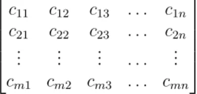
An approach to break the Zodiac-340 cipher using a combination of the Simple Substitutuion Columnar Transposition technique and the Jakobsen’s algorithm has been outlined in the research paper [20]. A major difference between the SSD and SSCT techniques is that in SSD, the plaintext and the ciphertext are a stream of characters, whereas in SSCT, they are represented as a matrix. If the initial ciphertext is represented as shown in Table 10, we need to store the digraph frequencies for every permutation of the columns. We should also note that when the matrix is flattened
Table 9: Final ciphertext matrix ⎡ ⎢ ⎢ ⎢ ⎢ ⎣ 𝑎 𝑑 𝑎 𝑏 𝑓 𝑑 𝑎 𝑐 𝑒 𝑐 𝑎 𝑓 ℎ 𝑔 𝑘 𝑎 𝑒 𝑗 𝑖 𝑔 𝑙 𝑚 𝑛 𝑎 𝑜 𝑑 𝑎 𝑖 𝑒 𝑎 𝑎 𝑗 𝑎 𝑔 𝑛 𝑖 𝑔 𝑘 𝑒 𝑔 𝑓 𝑥 𝑥 𝑔 𝑥 𝑥 𝑥 𝑥 𝑥 𝑘 ⎤ ⎥ ⎥ ⎥ ⎥ ⎦
Table 10: Initial ciphertext matrix ⎡ ⎢ ⎢ ⎢ ⎣ 𝑐11 𝑐12 𝑐13 . . . 𝑐1𝑛 𝑐21 𝑐22 𝑐23 . . . 𝑐2𝑛 ... ... ... . . . ... 𝑐𝑚1 𝑐𝑚2 𝑐𝑚3 . . . 𝑐𝑚𝑛 ⎤ ⎥ ⎥ ⎥ ⎦
out, the last element of the 𝑖𝑡ℎ row will be adjacent to the first element of the 𝑖+ 1𝑡ℎ
row. [20] describes a data structure to effectively store this information by parsing the ciphertext. Given a transposition key
𝐾 = (𝑘1, 𝑘2, 𝑘3, ...𝑘𝑛) the digraph matrix D is given by
𝐷=𝐷𝑘1,𝑘2+𝐷𝑘2,𝑘3+· · ·+𝐷𝑘𝑛−1,𝑘𝑛+𝐷𝑘𝑛,𝑘1′
where 𝐷𝑖,𝑗 is the digraph frequencies matrix when column 𝑗 is next to column 𝑖 and
𝐷𝑖,𝑗′ accounts for the digraph frequencies for the wrap around case
If we were to apply the Jakobsen’s algorithm directly to this case, then, during every iteration, we would need to swap the rows and columns for each 𝐷𝑖,𝑗 matrix. This would be time consuming. Instead, it is shown in [20] that swapping the rows and columns of the𝐸 matrix would yield the same score. Hence we avoid the cost of
recomputing the 𝐷 matrix during every iteration. With this modification, the steps
to compute the score for each putative key is given by:
∙ Assemble the 𝐷matrix from the already computed𝐷𝑖,𝑗 matrices, based on the key 𝐾
∙ s=∑︀
3.3 SSCT for Malware Detection
In order to use SSCT as a scoring technique for malwares, we need to represent the data from the known virus files, which we will refer to as the model, as the plaintext and the data from the file to be scored, as the ciphertext. In both the model and the file to score, we take only the 𝑘 top opcodes. All other opcodes are
categorized as ‘other’.
The 𝐸 matrix should reflect the digraph statistics of all the files in the model.
The algorithm to compute this matrix is given in Table 11. To build this matrix, we compute the normalized digraph frequencies for each file separately and sum up the individual matrices to get the final 𝐸 matrix. It should be noted that in this
approach, we have two keys—one corresponding to the opcode substitution and the other for the columns transposition in the matrix. We will denote the former as the substitutionKey and the latter as the transpositionKey.
Table 11: Compute 𝐸 Matrix
Initialize 𝐸 to 0
for each file in model
Initialize digraph matrix 𝑚 to 0
opcodeCurrent = readOpcode from file opcodeNext = readOpcode from file total= 0
while opcodeNext is not NULL
𝑚[opcodeCurrent][opcodeNext] + +
opcodeCurrent=opcodeNext
opcodeNext = readOpcode from file total+ +
end while
𝑚 =𝑚/total 𝐸 =𝐸+𝑚
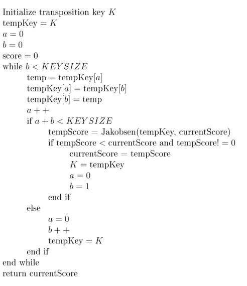
The opcodes from the file to be scored are populated in a matrix. This would be our ciphertext matrix 𝐶. We use this to compute the 𝐷𝑖,𝑗 matrices. We then guess an initial substitution key based on the opcode frequencies in the model and the file to score. The unknown file is scored using a nested hill climb approach against the model. The algorithm used to compute the score is outlined in Table 12. This function, in turn, calls the Jakobsen’s algorithm explained in Table 13.
Table 12: Compute Score Input: currentScore
Initialize transposition key𝐾
tempKey=𝐾 𝑎= 0 𝑏 = 0 score= 0 while 𝑏 < 𝐾𝐸𝑌 𝑆𝐼𝑍𝐸 temp=tempKey[𝑎] tempKey[𝑎] =tempKey[𝑏] tempKey[𝑏] =temp 𝑎+ + if 𝑎+𝑏 < 𝐾𝐸𝑌 𝑆𝐼𝑍𝐸
tempScore = Jakobsen(tempKey, currentScore) if tempScore<currentScore and tempScore! = 0
currentScore = tempScore 𝐾 =tempKey 𝑎= 0 𝑏= 1 end if else 𝑎= 0 𝑏+ + tempKey=𝐾 end if end while return currentScore
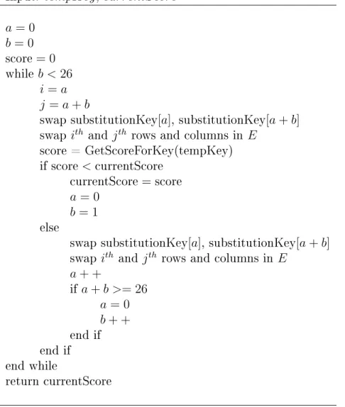
Table 13: Jakobsen’s Algorithm Input: 𝑡𝑒𝑚𝑝𝐾𝑒𝑦,𝑐𝑢𝑟𝑟𝑒𝑛𝑡𝑆𝑐𝑜𝑟𝑒 𝑎 = 0 𝑏 = 0 score = 0 while 𝑏 <26 𝑖=𝑎 𝑗 =𝑎+𝑏
swap substitutionKey[𝑎], substitutionKey[𝑎+𝑏]
swap𝑖𝑡ℎ and 𝑗𝑡ℎ rows and columns in𝐸
score = GetScoreForKey(tempKey) if score<currentScore currentScore=score 𝑎 = 0 𝑏 = 1 else
swap substitutionKey[𝑎], substitutionKey[𝑎+𝑏]
swap 𝑖𝑡ℎ and 𝑗𝑡ℎ rows and columns in 𝐸
𝑎+ + if 𝑎+𝑏 >= 26 𝑎= 0 𝑏+ + end if end if end while return currentScore
CHAPTER 4 Experiments and Results
Malware are categorized into several families based on their characteristics. As anyone would correctly assume, the response to any malware detection technique differs from one family to another. In this chapter, we will briefly describe the several malware families we have considered and present our experiments and their results. 4.1 Dataset
The SSCT implementation described in this project has been run on several malware families like Metamorphic Worm (MWOR), Next Generation Virus Creation Kit (NGVCK), Cridex, Security Shield, ZBOT, Smart HDD, Harebot and Winwebsec. A brief description of these families is given below.
∙ MWOR [12] is a type of worm that includes a metamorphic engine. This
meta-morphic engine is responsible in mutating the worm across generations, helping it to evade detection by security systems
∙ NGVCK is a self replicating, metamorphic virus. The NGVCK morphing engine
uses techniques like function ordering and dead code insertion to morph the virus [18]
∙ Cridex is a Trojan that spreads by infecting removable disk drives. It infects
the system by creating a backdoor entry point [9]
∙ Security Shield is a variant of the winwebsec family. It is a malicious software
Table 14: Dataset
Family Number of files
MWOR 100 NGVCK 50 Cridex 74 Security Shield 58 ZBOT 2136 Smart HDD 68 Harebot 53 Winwebsec 4360 Benign set 214
∙ ZBOT or Zeus is a trojan horse that steals information from infected systems
by techniques like form grabbing [17]
∙ Smart HDD is a virus that disables the security softwares in the infected
sys-tems [7]
∙ Harebot is a rootkit that uses keystroke logging to get unauthorized information
from the infected system
∙ Winwebsec is a malicious software that displays fake warning messages and
popups in the infected system [11]
Benign files used in the experiments for Linux malware were taken from several Linux utility programs like mv, cp, mkdir etc., Several Cygwin utility files were used as the benign files to score the malware files for Windows platform. The number of virus files in each family can be found in Table 14. All the files in each family were grouped into five sets and a five fold cross validation was done in order to obtain the malware and the benign scores.
4.2 Parameters
When we disassemble both the malware and the benign files, we find that they contain a large number of distinct opcodes. Of these opcodes, only a certain number of them appear consistently and contribute to the inherent malicious or benign nature of these files. All other opcodes occur quite infrequently and can collectively be categorized as the ‘other’ category. Hence, the opcode sequence of the files now contain the top 𝐾 frequently occurring opcodes and the ‘other’ opcodes. In the
previous research involving Simple Substitution Distance [8], it has been shown that taking the top 25 distinct opcodes yields the best results. Hence, in our experiments, we adopt the same value.
We have tried out three different approaches for our implementation. In the first approach, we use the same number of columns for all the test files and compute their scores. This is repeated for various column configurations, that is, all test files are scored by arranging them in a two column matrix first, then 5, 10 and so on. In the second approach, each file is scored using various number of columns and then the scores are collected for all test files. Since the scores did not differ from each other by a large margin, and since the first approach is faster, we have continued all further experiments using the first approach. The third approach uses Index Coincidence scores to find the correct column permutation and then uses a hill climb approach to arrive at the best possible substitution key. The difference between this and the first two approaches is that, in this approach, we separate the transposition and the substitution layers in our problem. We have tested this approach on a subset of Winwebsec files. Figure A.24 and Figure A.23 represent the ROC curve and the scatter plots for this approach.
the ciphertext matrix shown in Table 10. The number of columns taken were 2, 5, 10, 15, 20 and 25. Since the score obtained was the same in all these cases and since the running time is lesser when the number of columns is 2, we have continued all our experiments using that value.
4.3 Results
We obtained the malware and benign scores for the test data from the experi-ments we carried out on the different malware families. Using this data, we calculate the false positive and the false negative rates for each of the families and use them to plot Receiver Operating Characteristics curve (ROC curve) [5]. The area under the ROC curve (AUC value) is a value between 0 and 1, inclusive. This value gives the probability with which our system will correctly classify any random file as a malware or a benign file [3]. Table 15 gives a comparison of the AUC values for the different malware families obtained by using the SSCT, SSD and HMM tech-niques [1, 2, 16, 15, 14]. The visualization of the results in this table are provided through scatterplots and ROC curves for each of the families and are included in the Appendix A.
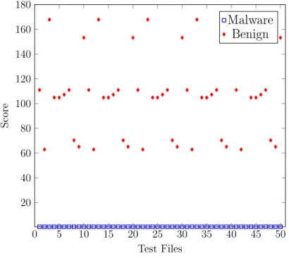
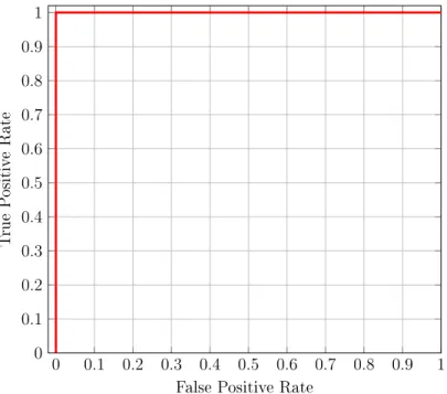
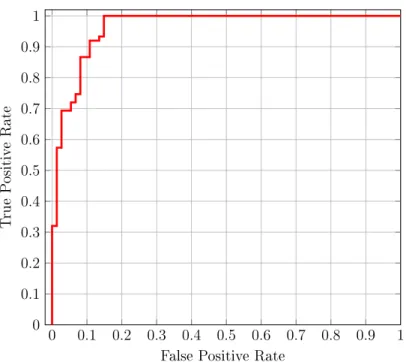
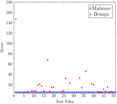
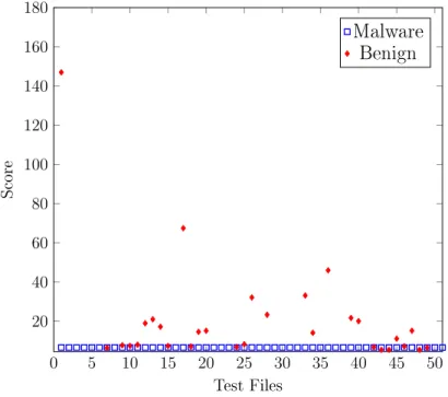
As we see from Table 15, for some families, the AUC value obtained using the SSCT technique is 1, which is the ideal value we strive for, and for a few others, the value drops. The AUC value of 1 is obtained when there is a clear demarcation between the malware and the benign scores. For example, from the scatterplot of these values for the family NGVCK given in Figure 1, we see that the range of values for the malware and benign scores do not overlap. As, a result, we have a perfect ROC curve with an AUC value of 1, as shown in Figure 2. On the other hand, in the case of the Cridex family of malware, there is some overlapping of the malware
Table 15: AUC values
Malware Family AUC using SSCT AUC using SSD AUC using HMM
MWOR0.5 0.51 1 1 MWOR1 0.58 1 0.99 MWOR1.5 0.70 0.9921 0.9625 MWOR4 0.80 0.9933 0.8225 NGVCK 1 1 1 Cridex 0.96288 0.58306 0.596 SecurityShield 1 0.62902 0.994 ZBOT 0.867 0.8664 0.9874 Smart HDD 1 0.8855 0.99875 Harebot 1 0.5606 1 Winwebsec 0.7328 0.8374 1
and the benign scores, as shown in Figure 3. This results in the ROC curve shown in Figure 4. The scatterplot and the corresponding ROC curves for the remaining families are included in the Appendix A.
0 5 10 15 20 25 30 35 40 45 50 20 40 60 80 100 120 140 160 180 Test Files Score Malware Benign
Figure 1: Scatter Plot NGVCK
0 0.1 0.2 0.3 0.4 0.5 0.6 0.7 0.8 0.9 1 0 0.1 0.2 0.3 0.4 0.5 0.6 0.7 0.8 0.9 1
False Positive Rate
True
Positiv
e
Rate
Figure 2: NGVCK ROC Curve
0 5 10 15 20 25 30 35 40 45 50 20 40 60 80 100 120 140 Test Files Score Malware Benign
0 0.1 0.2 0.3 0.4 0.5 0.6 0.7 0.8 0.9 1 0 0.1 0.2 0.3 0.4 0.5 0.6 0.7 0.8 0.9 1
False Positive Rate
True
Positiv
e
Rate
Figure 4: Cridex ROC Curve
the other techniques considered in the literature. We can attribute this performance improvement to two factors. First is the opcode substitution which is handled by the substitutionKey in our implementation. This addresses morphing techniques that replace opcodes with other interchangeable opcodes. It should be noted that the SSD technique also handles this case. The second, and the distinguishing factor, is the column transpositions in our ciphertext matrix, handled by the transpositionKey. Rearranging the columns in the matrix could account for morphing techniques that use sub-routine re-ordering and hence increase the detection rate in morphed malware. This might also be the reason causing this technique to not perform as well as the SSD method, in case of families like Winwebsec.
Another interesting fact to note from the results is that, when we observe the scatter plots in Figure A.5 to Figure A.8 in Appendix A for the different padding ratios in the MWOR family, the gap between the benign and the malware scores
seems to increase with the increase in the padding ratio. This can be due to the fact that as more and more dead code is inserted, the malware files become more similar to one another than to the benign files.
CHAPTER 5
Conclusion and Future Work
In this project we have implemented the SSCT algorithm to score several malware families. Our implementation takes a set of training files and builds a model out of those files. This model is then used to score a set of test files, which may be benign or malign. One of the challenging aspects of this project was to represent the information from all the files in the training set, in the model. We have used five fold cross validation to ensure that the results are unbiased. Our experiments were carried out on several hundreds of malware files across different families and this has given us a chance to observe how each of these families reacts to this scoring technique. In addition to the SSCT module, we have also implemented the SSD technique to compare our scores and to verify the correctness of our implementation.
On comparing the SSCT scores with the scores from previous researches like the Simple Substitution Distance for malware detection, we see that the SSCT technique gives better results in many families.
This project has sufficient scope for future research and optimization. Currently, we observe an increase in the running time of the module when the number of columns is increased. This aspect has definite room for improvement and any future work can attempt to optimize the running time of the algorithm. Another aspect that could be improved is the performance of the SSCT technique on families like Winwebsec and MWOR, where the detection rate is lower than that of the rate for the SSD method. We can try out different swapping techniques for the substitution key and the transposition key as discussed in [8] and compare the AUC values obtained in
each case. In this project, except for the MWOR family, we have not taken the padded variants of other families. It would be interesting to see if the SSCT method continues to detect these other families even with increased padding ratios.
LIST OF REFERENCES
[1] C. Annachatre, T. H. Austin, M. Stamp, Hidden Markov Models for Malware Classification, Journal of Computer Virology and Hacking Techniques, 11(2):59– 73, May 2015
[2] T. Austin, E. Filiol, S. Josse, M. Stamp, Exploring Hidden Markov Models for Virus Analysis, A Semantic Approach, Proceedings of the 46th Hawaii International Conference on System Sciences, 5039–5048, January 2013
[3] A. P. Bradley, The Use of the Area Under the ROC Curve in the Evolution of Machine Learning Algorithms, Pattern Recognition, 30:1145–1159, 1997
[4] A. Dhavare, R. M. Low, M. Stamp, Efficient Cryptanalysis of Homophonic Sub-stitution Ciphers, Cryptologia, 37:250–281, 2013
[5] T. Fawcett, An Introduction to ROC Analysis, Pattern Recognition Letters, 27(8):861–874, 2006
[6] T. Jakobsen, A Fast Method for the Cryptanalysis of Substitution Ciphers, Cryp-tologia, 19:265–172, 1995
[7] Kaspersky–Rogue Security Software, http://support.kaspersky.com/ viruses/rogue?qid=208286454, Accessed November 2015
[8] R. M. Low, G. Shanmugam, M. Stamp, Simple Substitution Distance and Metamorphic Detection, Journal of Computer Virology and Hacking Techniques, 9(3):159–170, March 2013
[9] Microsoft Malware Protection Center, Cridex, http://www.microsoft.com/ security/portal/threat/encyclopedia/entry.aspx?Name=Win32%2FCridex, Accessed November 2015
[10] Microsoft Malware Protection Center, SecurityShield, http://www. microsoft.com/security/portal/threat/encyclopedia/Entry.aspx?Name= SecurityShield, Accessed November 2015
[11] Microsoft Malware Protection Center, Winwebsec, https://www.microsoft. com/security/portal/threat/encyclopedia/entry.aspx?Name=Win32%
2fWinwebsec, Accessed November 2015
[12] S. M. Sridhara, Metamorphic worm that carries its own morphing engine, http://citeseerx.ist.psu.edu/viewdoc/download?doi=10.1.1.344. 549&rep=rep1&type=pdf, 2012
[13] M. Stamp, Information Security: Principles and Practice, second edition, Wiley, 2011
[14] T. Singh, Support Vector Machines and Metamorphic Malware Detection, http: //scholarworks.sjsu.edu/etd_projects/409/, 2015
[15] S. Vemparala, Malware Detection Using Dynamic Analysis, http: //scholarworks.sjsu.edu/cgi/viewcontent.cgi?article=1403&context= etd_projects, 2015
[16] M. Stamp, W. Wong, Hunting for Metamorphic Engines, Journal in Computer Virology, 2:211–229, 2006
[17] Symantec Security Response, ZBOT, http://www.symantec.com/security_ response/writeup.jsp?docid=2010-011016-3514-99, Accessed November 2015 [18] P. Szor, The Art of Computer Virus Research and Defense, Pearson Education,
2005
[19] W. Williamson, Evolution of Malware, http://www.securityweek.com/ evolution-malware, Accessed November 2015
[20] J. Yi, Cryptanalysis of Homophonic Substitution-Transposition Cipher, http://scholarworks.sjsu.edu/cgi/viewcontent.cgi?article=1359&
APPENDIX Experiments
In this section, we provide the scatterplots and the ROC curves for all the families we have experimented on. When running the experiments on each of the families, we recorded the malware scores and the benign scores and used these to generate the scatterplots shown in figures A.5 to A.13. From these scores, we calculated the true positive and the false positive rates and used them to generate the ROC curves shown in figures A.14 to A.22. The ROC curves given here correspond to the AUC values displayed in Table 15. 0 5 10 15 20 25 30 35 40 45 50 20 40 60 80 100 120 140 160 180 Test Files Score Malware Benign
0 5 10 15 20 25 30 35 40 45 50 20 40 60 80 100 120 140 160 180 Test Files Score Malware Benign
Figure A.6: Scatter Plot MWOR 1
0 5 10 15 20 25 30 35 40 45 50 20 40 60 80 100 120 140 160 180 Test Files Score Malware Benign
0 5 10 15 20 25 30 35 40 45 50 20 40 60 80 100 120 140 160 180 Test Files Score Malware Benign
Figure A.8: Scatter Plot MWOR 4
0 5 10 15 20 25 30 35 40 45 50 20 40 60 80 100 120 140 160 180 Test Files Score Malware Benign
0 5 10 15 20 25 30 35 40 45 50 10 20 30 40 50 60 70 80 Test Files Score Malware Benign
Figure A.10: Scatter Plot ZBOT
0 5 10 15 20 25 30 35 40 45 50 20 40 60 80 100 Test Files Score Malware Benign
0 5 10 15 20 25 30 35 40 45 50 10 20 30 40 50 60 70 80 Test Files Score Malware Benign
Figure A.12: Scatter Plot Harebot
0 500 1,000 1,500 2,000 2,500 3,000 3,500 4,000 10 20 30 40 50 60 70 Test Files Score Malware Benign
0 0.1 0.2 0.3 0.4 0.5 0.6 0.7 0.8 0.9 1 0 0.1 0.2 0.3 0.4 0.5 0.6 0.7 0.8 0.9 1
False Positive Rate
True
Positiv
e
Rate
Figure A.14: MWOR0.5 ROC Curve
0 0.1 0.2 0.3 0.4 0.5 0.6 0.7 0.8 0.9 1 0 0.1 0.2 0.3 0.4 0.5 0.6 0.7 0.8 0.9 1
False Positive Rate
True
Positiv
e
Rate
0 0.1 0.2 0.3 0.4 0.5 0.6 0.7 0.8 0.9 1 0 0.1 0.2 0.3 0.4 0.5 0.6 0.7 0.8 0.9 1
False Positive Rate
True
Positiv
e
Rate
Figure A.16: MWOR1.5 ROC Curve
0 0.1 0.2 0.3 0.4 0.5 0.6 0.7 0.8 0.9 1 0 0.1 0.2 0.3 0.4 0.5 0.6 0.7 0.8 0.9 1
False Positive Rate
True
Positiv
e
Rate
0 0.1 0.2 0.3 0.4 0.5 0.6 0.7 0.8 0.9 1 0 0.1 0.2 0.3 0.4 0.5 0.6 0.7 0.8 0.9 1
False Positive Rate
True
Positiv
e
Rate
Figure A.18: SecurityShield ROC Curve
0 0.1 0.2 0.3 0.4 0.5 0.6 0.7 0.8 0.9 1 0 0.1 0.2 0.3 0.4 0.5 0.6 0.7 0.8 0.9 1
False Positive Rate
True
Positiv
e
Rate
0 0.1 0.2 0.3 0.4 0.5 0.6 0.7 0.8 0.9 1 0 0.1 0.2 0.3 0.4 0.5 0.6 0.7 0.8 0.9 1
False Positive Rate
True
Positiv
e
Rate
Figure A.20: SmartHDD ROC Curve
0 0.1 0.2 0.3 0.4 0.5 0.6 0.7 0.8 0.9 1 0 0.1 0.2 0.3 0.4 0.5 0.6 0.7 0.8 0.9 1
False Positive Rate
True
Positiv
e
Rate
0 0.1 0.2 0.3 0.4 0.5 0.6 0.7 0.8 0.9 1 0 0.1 0.2 0.3 0.4 0.5 0.6 0.7 0.8 0.9 1
False Positive Rate
True
Positiv
e
Rate
Figure A.22: Winwebsec ROC Curve
0 20 40 60 80 100 120 140 160 180 200 0 0.2 0.4 0.6 0.8 1 1.2 1.4 1.6 1.8 2 Test Files Score Malware Benign
0 0.1 0.2 0.3 0.4 0.5 0.6 0.7 0.8 0.9 1 0 0.1 0.2 0.3 0.4 0.5 0.6 0.7 0.8 0.9 1
False Positive Rate
True
Positiv
e
Rate