Defence Science Journal, Vol. 66, No. 2, March 2016, pp.138-145, DOI : 10.14429/dsj.66.9701 2016, DESIDOC
1. IntroductIon
Malware is an all-encompassing term which encapsulates all program created with intent to cause harm to computer systems and includes viruses, worms, trojans among others. The loss caused to the computer systems and their users due to these malware can be in the form of loss of sensitive information, system downtime, reduced performance and loss of reputation.
Most of the antivirus softwares use signature based techniques for malware detection that involves matching the files to be checked for infection against a database containing the malware signatures. This requires a signature to be generated for each malware and can be easily evaded. The newest forms of malware employ code obfuscation techniques such as register renaming, code reordering, instruction replacement, garbage code insertion and semantic nops which change the signature of the malware while keeping the intended functions intact. This helps the malware to evade the antivirus software and continue spreading till such time its signature is generated. These types of malwares are called as metamorphic malware and have metamorphing engines built in their code allowing the malware to create multiple variants of it. Detection of metamorphic malwares is still an open challenge.
To overcome the challenges posed by metamorphic malware, research has been done for their detection through various techniques. Some of these techniques focused on API calls, some on function calls made by malware while some used control flow graphs. All these techniques can be broadly classified into dynamic and static detection techniques. Dynamic detection techniques involve executing the malware in a protected environment and examining its run-time behaviour. The focus is on analysis of API calls made, actions being taken by the malware such as create process,
registry changes, file changes etc. Such detection techniques can examine packed or polymorphic malware. Static detection techniques involve examining the malware without executing the program. Static detection analyse the content using header information, control flow graphs, opcodes and API call graphs etc and ensures complete code coverage and can reveal all possible actions a malware may carry out; while dynamic detection will only reveal information about what the malware is doing at that time. Existing CFG and Opcodes sequence based malware detection methods either cannot accurately describe the behaviours of the original executables or based on binary classification only. The remarkable growth in malware and benign apps needs automated analysis of potentially dangerous apps to aid malware analysts. In the real world scenario, it would be extremely helpful to be informed of the type as well as the family of the malware. The groupings of the samples into families in turn help to establish the relationships among them, identify the potential source of infection, detect the newer variants and study the advancement of the a variety of known malwares.
2. rELAtEd WorK
Use of machine learning technique for malware detection was proposed by Schultz1, et al. Their experimental results indicated to achieve good detection rates compared to the traditional signature based methods. Kolter2, et al. improved the results by using n-grams of the opcode sequences as features which are extracted from executables. Bruschi3, et al. first proposed the use of CFG for detection of self-mutating malware along with graph matching techniques. Bilar4, et al. proposed malware detection method based on opcode distributions in malware and benign which differed significantly. Igor5, et al. and Robert6, et al. used opcode sequences to represent program
control Flow Graph Based Multiclass Malware detection
using Bi-normal Separation
Akshay Kapoor
*and Sunita Dhavale
*Department of Computer Engineering, Defence Institute of Advanced Technology, Girinagar - 411 025, India *E-mail: [email protected]
ABStrAct
Control flow graphs (CFG) and OpCodes extracted from disassembled executable files are widely used for malware detection. Most of the research in static analysis is focused on binary class malware detection which only classifies an executable as benign or malware. To overcome this issue, CFG based multiclass malware detection system that automatically classifies the malware into their respective families is proposed. The use Bi-normal separation (BNS) as a feature scoring metric. Experimental results show that proposed method using BNS outperforms compared to hitherto use technique of document Frequency for multiclass metamorphic malware detection and achieves detection accuracy of 99.5 per cent.
Keywords: Bi normal separation, control flow graph, machine learning, malware detection
behaviour and applied machine learning methods for malware detection. Igor5, et al. used static analysis to extract opcode sequences in the order of their appearance in a decompiled executable.
Zhao7, et al. has extracted all opcode sequences from basic blocks of an executable. They separated a decompiled executable into basic blocks, and then extracted the opcode sequences from basic blocks. These opcode sequences were used to represent program behaviour and the authors used machine learning to detect malware. however, as the basic blocks were only considered and not the execution order among these basic blocks, the control flow information was not captured in its entirety8.
Ding8, et al., considered opcode sequences from all execution paths (path from root to leaf) and extracted n-grams from the opcode stream. For feature extraction, unique n-grams are used as features. Machine learning is used to detect malware by using document frequency threshold for feature selection. Their malware detection model is designed for binary class detection wherein the files get classified as malware or benign. This may not completely useful in the real world scenario where the user has to be informed of the type as well as the family of the malware, to help identify the potential source of infection and also to detect the newer variant of an existing malware.
Forman9, proposed the use of Bi normal separation as a feature selection metric for text classification. BNS is used for feature scaling for text classification10. The experimental results showed that use of BNS provided better results over TF-IDF for text classification especially in skewed class datasets where number of samples for one class was very large as compared to the samples in the other class.
Authors research closely follows the work ofDing8, et al. and employs the use of BNS for feature scoring and using chi-square test for feature selection to detect malware families. This helps in to differentiate between the families and detect unknown variant of a known malware. They concentrated their efforts towards detecting malware in the windows OS. 3. ProPoSEd ModEL
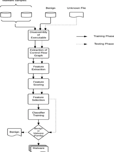
The proposed multiclass malware detection system consists of training and testing phase as shown in Fig. 1. 3.1 disassembly of Executable
Before any executable file is analysed, it needs to be disassembled first. We used IDA Pro15, a commercially available recursive loop disassembler to disassemble the executable. Since, static analysis cannot be done on packed files, we need to check whether the file is packed i.e. either compressed or encrypted or both, as a packed file will reveal no information. we used PEId software16, to check for packing as well as the type of packer used. If a file is found to be packed, it is first unpacked using corresponding unpacker eg UPX17, before it is disassembled.
3.2 control Flow Graph Extraction
Most of the programs including malware run by executing instructions, making API calls, calling subroutines and making
changes to the system, either temporary or permanent. The instructions executed by a program can be broadly classified based on the type of actions being performed by them, some move data between various locations, some carry out mathematical operations while some transfer the control between different blocks of code. The class of instructions that transfers the control between different blocks of code within the program helps in creation of control flow graphs.
Proposed system uses IDA pro to disassemble the file and generate the control flow graph of the executable with each basic block having a unique block id, start and end addresses and its successors if any. Generated CFG represents all paths which can be traversed through a program during execution and is a weighted directed graph. It contains nodes and edges, where each node contains the instructions to be executed while edges denote the transfer of control between two blocks of code. If control can be passed from one node to another, then there exists an edge between the two nodes with direction of the edge indicating the flow of control.
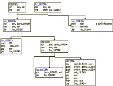
Each node in the control flow graph is known as a basic block. A basic block has the property of having single entry and exit points. It implies that if the first instruction of the basic block is executed then all the instructions of the block will be executed sequentially. Figure 2 shows a portion of the control flow graph of calculator program (benign file) from the system 32 folder of windows 7 OS.
By analysing the control flow graph, we can capture the behaviour of an executable. After a file has been disassembled,
the control flow information needs to be extracted. The information is extracted from IDA Pro using a custom script written in Python which accesses IDA Pro APIs to extract the information which includes unique id of each basic block, its start and end addresses, all the instructions contained in the basic blocks and its successor blocks. Once the information about the basic block is extracted, a tree is created to depict its control flow and all possible execution traces recorded. It is important to avoid loops as considering loops will lead to indefinitely long execution paths. Capturing all possible execution traces provides us the correct behaviour of the executable. These execution traces are then concatenated and saved as the execution profile of the executable. A data structure is used to store basic block information as shown below:
( ) ( ) ( ) ( int ) ( int ) BlockID Numeric StartAddr Hex ClassTreeNode EndAddr Hex
LeftChild Po er RightChild Po er
The Tree Nodes stores BlockID, which is the unique ID for each Basic block of the executable. StartAddr and EndAddr store the starting and end address of the particular basic block. LeftChild and RightChild store the pointers to the successor nodes, if any of that block. Besides these, certain methods were defined to initialise the node with the relevant information, a method to read all the instructions and a method to store the pointers to the successor nodes.
To extract the control flow and all the possible execution traces a modified depth-first tree traversal algorithm is used which apart from storing all the traversed nodes also carried out the check for loops and discard them as and when encountered. The pseudo code is depicted as Algorithm 1.
1:
Algorithm ExtractExecutionPath
: Node( )
Input Start Basic BlockID
: ( )
Output ArrayofExecutionTrace Basic BlockIDs
: [], ExecPath[], ExecPath[]
DefineArrays Stack Curr Total Algorithm :
1. Counter=0
2. Push StartNode on Stack
3. While Stack!=Empty do
4. Pop Stack
5. CurrExecPath =CurrExecPath ∪ Basic BlockID
6. Counter Counter= +1
7. If Exists RightChild( ) and RightChild Curr⊄ ExecPath 8. Push RightChild on Stack
9. PathLen=PathLen+Counter
10. endif
11. If NotExists LeftChild( ) and LeftChild Curr⊂ ExecPath
12. TotalExecPath =TotalExecPath+CurrExecPath
13. Delete nodes from Curr_ _ ExecPath till last added RightChild_ _
14. Adjust Counter_
15. Elseif Exists LeftChild( ) and LeftChild Curr⊄ ExecPath 16. Push LeftChild on Stack
17. endif
18. endwhile
19. Return TotalExecPath
Figure 3 shows the basic block IDs of the execution trace of sample control flow graph. All the execution paths are concatenated. The numbers shown are the IDs of the basic blocks executed in order
Figure 2. Control flow graph of calc.exe.
Figure 3. Execution trace of calc.exe shown by basic block Ids.
Figure 4. opcode sequences extracted from the execution trace.
The opcode sequence trace are extracted from the execution trace by traversing through each basic block in the order of its execution as extracting all the while discarding any operands as shown in Fig. 4. The process of extracting the complete execution trace is computationally intensive which requires machine with good processing capabilities.
3.3 Feature Extraction
Manning11, et al. had proposed the use of n-grams as features and the same is a widely used technique in natural language processing as well as document classification. n-gram method means selecting a group of words as features for classification or sentiment analysis with n representing the number of words in each feature. 3-grams (trigrams) as for features as experimentally shown to be most effective8. For
feature extraction we use sliding window approach, as used by8 and generate the trigrams, Figure 5. Each of these trigrams is a feature with all the trigrams of an executable being the feature vector. Two different approaches for feature set are used. In the first approach all trigrams from the execution trace were considered and in the second approach only the unique trigrams were taken. These extracted trigrams form text documents for corresponding malwares.
1 or 0, hence they are restricted between 0.0005 and 1-0.0005 as proposed9,10.
Term frequency-inverse document frequency (tfidf), is a numerical statistic to find out how important a word is in a set of documents. It is obtained by multiplying the term frequency of the feature with the inverse of its document frequency and is given by the Eqn. (3):
( )i ( , )i j ( , )i
tfidf f =tf f d ×idf f D (3) where
( , )i j
tf f d Number of times a feature is present in the documentdj.
( , )i
idf f D Inverse of the document frequency given by log N
D
N Total number of documents.
D Number of documents in which feature fi is present.
Term frequency Bi-normal separation (TF.BNS)
proposed10, is calculated by multiplying the term frequency of the feature with its BNS score as given in Eqn. (4):
. ( )i ( , )i j ( )i
TF BNS f =tf f d ×BNS f (4) Ding8, et al. used DFfor feature scoring and selected the top features based on document frequency score for each class after filtering out any features common to both classes. In our view, mere presence of a feature in different classes is not enough for it to be discarded and may lead to loss of some good features. we assign score to each feature and use an independent metric for feature selection. This has shown good results in the classification results.
3.5 Feature Selection
Feature selection is carried out to convert the feature set to a manageable size and reduce the dimensionality of the features set to remove redundant and noisy feature which reduce the performance of the classification. Here, we carry out feature selection via filtering and have used two feature selection metrics which are commonly used. They are defined as:
Information gain (IG), gives out the decrease on entropy for any feature caused due to it being present or absent in a document class and is widely used as feature selection metric7,8,13. It is given by Eqn. (5):
| 0 {0,1} 0 | | ( , ) ln ln | | j q j m i j i q i i i C IG f C C C C C C = = = =
∑
− −∑
∑
− (5) where fm mthfeature. C Number of documents. j Number of classes.Ci Number of documents belonging to class i. Cq| Number of documents containing the feature fm Ci Number of documents of class i containingfm.
q Presence or absence of a feature. It can be either 0 if absent or 1 if present.
Chi-Square (χ2) test : The χ2test is used to test the
Figure 5. Extracted 3-grams to be used as features.
3.4 Feature Scoring
Before classification, these documents need to be converted from text form to vector space representation in matrix form where each row represents a document and each column represents the features. The total number of columns is the total number of features extracted from the documents.
To enable classifier to effectively differentiate between the various classes, feature scaling is done to give a numerical value to each of these features. Various techniques are used for feature scaling. Some of the techniques are defined as follows.
Document frequency (DF) of a feature fives the number of documents the feature occurs in a class of documents12, and is given by the Eqn. (1):
lg ( , ) lg p i j j C DF f C C = (1)
whereDF f C( , )i j is document frequency of the ithfeature in th
j class of documents, Cp: Number of documents of class j,
which contain the feature. j
C : Number of documents of class j, i : index of the feature extracted(i N N∈ ), is the total number of features. j : Number of classes ie. Benign and different malware families.
Bi-normal separation (BNS) measures the importance of a feature based on its presence in different classes of documents9,10 and is given by Eqn. (2):
1 1 1 ( ) p N i j j C C BNS f F F C C− − − = − (2) whereF−1is the inverse cumulative probability function of standard normal distribution.
p j C C
: True positive rate for a feature.
1 N j C C−
: False positive rate for the feature.
Since BNS scores are calculated over binary classes, one vs rest all classes approach to signify positive and negative classes is used. It is important to note that the BNS score will tend to ∞ if either of the true positive rate or false rate becomes
independence of two variables. The χ2test measures the independence of a feature and a category. Features with the higher χ2 values are less independent for a category, and bound to perform better for classification13. It is given by the
Eqn. (6). 2 2 1 ( ) ( ) n i i i i i O E f E = − χ =
∑
(6) where Oi is observed value of feature i, Eiis expected value of feature i.3.6 training and testing
The detection method uses machine learning for classifying a file into benign or the respective malware family. The process consists of two steps: training and testing. In the training phase, the classifier requires to be trained to be able to differentiate between malware and benign files and involves using a training dataset of feature vectors to be used alongwith the class labels for building the classification model. In the testing phase, unlabelled dataset is passed to trained model to evaluate the performance of the classification model.
For the purpose of evaluating our approach, we used two different techniques for training and testing the classifiers. In the first approach we split up the dataset set into training and testing dataset with 80 per cent samples being used to train the classifier and rest 20 per cent for testing the classifier. We also used 10 fold cross validation where the entire dataset is randomly split up into 10 blocks with 9 blocks being used for training and the remaining block used for testing. This is then repeated 10 times.
We use multiple classifiers in our research. Some of the classifiers are as follows:
Naïve Bayes Classifier: It uses probabilistic methods to
assign classes to a document and is used in fields of information retrieval, text classification. We used two algorithms for the classifier using Gaussian distribution and multinomial distribution1.
Support Vector Machines14: They are non-probabilistic classifiers and used binary classification. We used one vs rest approach for multiple class classification as well as two class classification. Support Vector Machines (SVM) classify by representing features as points in multidimensional space and then separates out the different classes using maximum margin hyperplanes. We used three kernel functions for the SVM and include linear, polynomial and radial basis function.
Random Forest Tree Classifier (RF Tree): It is an ensemble
classifier which classifies by creating multitude of decision trees with features selected randomly from the feature space. we implemented our approach using python and made use of sklearn21, machine learning package of python. To compare the results with Ding8, et al, a well-known data mining tool Weka18 was used.
4. EXPErIMEntAtIon 4.1 Experimental Setup
To check the effectiveness of proposed method a number of experiments were carried on a machine with Intel i5 processor @ 3.1GHz clock speed, with 4GB RAM and windows 7 OS with Weka and Python interpreter installed.
4.2 data Set collection
For the experimentation, we collected 266 files from the system 32 folder of a freshly installed win 7 OS. The files were checked for any infection by uploading them to virustotal.com which checks the files uploaded using a number of antivirus software. The 133 malware samples were downloaded from vxheavens19 and openmalware20 repositories. The samples consisted of metamorphic virus, worms and generic Trojan agents. Two datasets were created for the experimentation. Dataset1 consisted of 266 benign and 105 metamorphic malware samples belonging to different families and Dataset2, created to check the performance of the proposed model against generic malware included generic Trojans apart from those in Dataset1.
4.3 Evaluation criteria
Both 10 fold cross validation as well standard split dataset techniques to measure the performance of the proposed model using BNS against DF for feature scaling were employed. Cross validation was done primarily to compare results of our model with the model proposed by Ding8, et al.
The performance of classifier was measured using three metric: accuracy, precision and recall. The same are defined as follows.
Accuracy: It is the ratio of correct results against the total results and calculated using Eqn. (7):
TP TN Accuracy TP TN FP FN + = + + + (7) Precision: Also known as positive predictive value, it gives ability of the classifier to correctly label the positive classes. It is calculated using Eqn. (8).
TP Precision
TP FP
=
+ (8)
Recall: It gives the sensitivity of the classifier and signifies the ability of the classifier to find all positive samples. It is calculated using the Eqn. (9).
TP Recall
TP FN =
+ (9) where TP is number of positive classes correctly classified as positive, FP is number of negative classes incorrectly classified as positive, TN is number of negatives classes correctly classified as negative, FN is number of negatives classes incorrectly classified as positive.
4.4 Experimental results
The malware detection method explained in Section 3 was implemented in python language. As mentioned earlier, we created two datasets for evaluating our approach. Extracted the features using the technique similar to Ding8, et al. From the execution trace, extracted all trigrams as well as unique trigrams. The dataset containing all trigrams was used for calculation of TF.BNS and TF-IDF scores, while unique trigrams were used for calculation of BNS and DF scores.
Ding8, et al. had selected features based on information gain (IG) and DF threshold. Classification results obtained
when using IG, DF threshold, and Chi-square test as feature selection technique are compered. Tables 1 - 3 show the average accuracy, precision and recall rates from different classifiers on Dataset1 over 5 iterations when using 80 per cent of the data set for training and 20 per cent for testing. we used chi square test for feature selection when using TF-IDF, TF.BNS, BNS and IG, Chi-square and DF threshold when using DF. The classifiers were trained and tested on different number of features to evaluate the performance of the classifier when using different number of features.
In the Tables 1 - 3; GNB, MNB, lSVC, PSVC, RBF and RF depict the classifiers Gaussian Naïve Bayes, Multinomial Naïve Bayes, Linear SVM, Polynomial SVM, SVM using Radial Basis function, and Random forest trees. The rates shown are expressed in percentage.
GnB MnB LSVc PSVc rBF rF TF.IDF 98.02 81.44 99.61 68.85 68.85 93.37 TF.BNS 98.36 74.42 99.9 68.85 99.71 98.71 BNS 98.7 98.46 99.54 90.28 99.41 98.73 DF-IG 93.64 94.49 93.18 86.20 92 91.03 DF-ChI 93.67 94.8 93.41 86.76 91.78 90.88 DF 90.14 94.2 94.36 80.28 80.28 94.36
table 1. Accuracy rates for dataset1
table 2. Precision rates for dataset1
GnB MnB LSVc PSVc rBF rF TF.IDF 98.22 82.45 99.64 47.41 47.41 98.34 TF.BNS 98.99 70.85 99.9 68.85 94.73 98.24 BNS 98.85 99.12 99.57 91.60 99.17 98.76 DF-IG 95.5 95.3 93.8 89.2 92.88 92.08 DF-ChI 95.2 95.25 94 88.9 92.69 91.99 DF 90.14 94.9 94.7 80.3 64.5 94.7
table 3. recall rates for dataset1
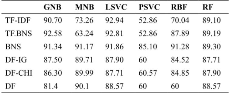
GnB MnB LSVc PSVc rBF rF TF.IDF 98.02 81.44 99.61 68.85 88.85 98.37 TF.BNS 98.36 74.42 99.9 68.85 94.71 98.17 BNS 98.70 98.46 99.54 90.28 99.11 98.73 DF-IG 93.67 95 93.16 87.26 92.02 91.01 DF-ChI 93.65 94.87 93.42 86.78 91.8 91.3 DF 90.10 94.2 94.4 64.5 80.3 94.4 GnB MnB LSVc PSVc rBF rF TF-IDF 90.70 73.26 92.94 52.86 70.04 89.10 TF.BNS 92.58 63.24 92.81 52.86 87.89 89.19 BNS 91.34 91.17 91.86 85.10 91.28 89.30 DF-IG 87.50 89.71 87.90 60 84.52 87.71 DF-ChI 86.30 89.99 87.71 60.57 84.85 87.90 DF 81.4 90.1 88.57 60 60 88.57
table 4. Accuracy rates for dataset2
table 5. Precision rates for dataset2 GnB MnB LSVc PSVc rBF rF TF-IDF 94.49 75.28 93.18 27.94 63.33 90.80 TF.BNS 93.92 56.22 93.64 27.94 90.19 90.70 BNS 92.45 91.18 92.91 88.40 92.51 91.3 DF-IG 92.6 90.82 86.50 36 82.60 86.7 DF-ChI 91.81 91.59 86.24 36.9 81.2 86.84 DF 82.5 90 88.57 36 36 87.5
table 6. recall rates for dataset2
GnB MnB LSVc PSVc rBF rF TF-IDF 90.70 73.26 92.24 52.86 70.04 89.10 TF.BNS 92.58 63.24 92.81 82.86 87.89 89.25 BNS 91.34 91.17 91.86 85.10 91.28 89.35 DF-IG 87.5 89.69 87.90 60 84.67 87.72 DF-ChI 86.45 89.57 87.41 54.18 84.86 87.1 DF 81.4 90.1 88.1 60 60 88.6
TF-IDF, TF.BNS, and BNS with chi-square feature selection gave best results with linear SVM giving accuracies of 99.61 per cent, 99.9 per cent, and 99.54 per cent, respectively with similar precision and recall rates, while DF with IG, chi-square and threshold as frequency selection metrics had best results with Multinomial Naïve Bayes classifier, giving accuracy results of 94.49 per cent, 94.8 per cent, and 94.2 per cent.
Tables 4 - 6 show the accuracy precision and recall rates for the same classifiers on Dataset2.
The performance for all feature scoring techniques dipped
for Dataset2 due to addition of generic malware Trojans which did not belong to any family. however, TF-IDF, TF.BNS and BNS still performed better than DF by around 3 per cent improvement in accuracy rates.
It can be seen, that TF-IDF and TF.BNS showed slightly better results as compared to BNS and DF. however, they both suffer from additional computational and storage overheads incurred while storing and processing all the trigrams present. hence, it is recommended to use only unique trigrams extracted. For the next set of experimentation by means of 10 fold cross-validation, we used only BNS and DF for classification tests. Figures 6 and 7 give the accuracy rates for BNS using chi square test for feature selection and DF scoring using DF threshold for feature selection8, using Gaussian Naïve Bayes, Linear SVM, SVM with radial basis function as kernel functions for dataset1 and dataset2, respectively.
It is seen from the figures above that BNS has performed consistently better than DF for multi-class malware detection, with average accuracies for BNS with GNB, lSVC and RBF being 97.38 per cent, 95.9 per cent, and 96.9 per cent, respectively for Dataset1 and 90.93 per cent, 92.33 per cent, and 93.2 per cent, respectively for Dataset2. Yuxin8, et al. had developed the model for only binary class classification. Our model when tested on binary class classification with all malwares combined into a single class gave average accuracy rates of 99.2 per cent with Gaussian
Naïve Bayes and SVM classifiers, indicating that most of misclassifications in our took place between different malware classes. The same was also confirmed by analysis of the confusion matrix generated at each stage.
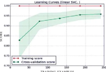
The learning curves for Gaussian Naïve Bayes and Linear SVM classifiers for the experiments involving BNS as feature scoring technique are shown by Figs. 8 and 9, respectively. Both the curves show that the classifiers have been trained and the test accuracy scores will improve as more samples are added. This will result in further improvement in detection accuracy as the number of malware samples increases.
5. concLuSIonS
Existing CFG and Opcodes Sequence based malware detection methods either cannot accurately describe the behaviors of the original executables or based on binary classification only. In this research paper, we have proposed an automated multiclass malware detection method using opcodes generated from CFGs and BNS for feature scoring. Our experimental results show an improvement of up to 4 per cent in accuracy, precision and recall rates over DF when tested over multiple classifiers. The proposed detection model also showed accuracy rates of 99.2 per cent for two class malware detection when using Gaussian Naïve Bayes and Support Vector Machines, which is much higher than what could be achieved using Document Frequency. The technique of scoring features performs better for classification than the filtering method of removing any features common to different classes of samples. Besides good performance, our proposed model achieves automatic classification of unknown malware samples into candidate families. This feature could be remarkably useful for malware analysts. Proposed method is bounded by the limitations that of any static detection technique.
rEFErEncES
1. Schultz, M.; Eskin, E.; Zadok, E. & Stolfo, S. Data mining methods for detection of new malicious executables. In
Proceedings of the IEEE Symposium on Security and Privacy, los Alamitos, CA, 2001. pp.38–49.
doi: 10.1109/SECPRI.2001.924286
2. Kolter Jeremy, Z. & Marcus, Maloof. learning to detect malicious executables in the wild. In Proceedings of the 10th ACM SIGKDD International Conference on Knowledge discovery and data mining, 2004, pp.470-478,
doi:10.1145/1014052.1014105
3. Bruschi, Danilo; lorenzo, Martignoni & Mattia, Monga. Detecting self-mutating malware using control-flow graph matching. In Proceedings of the Third international conference on Detection of Intrusions and Malware & Vulnerability Assessment, Springer Berlin heidelberg, 2006, pp.129-143.
doi:10.1007/11790754_8
Figure 6. comparative accuracy rates for dataset1.
Figure 7. comparative accuracy rates for dataset2.
Figure 9. Learning curve for Linear SVM classifier.
TRAINING EXAMPLES
SC
OR
E
Figure 8. Learning curve for Gaussian Naïve Bayes classifier.
TRAINING EXAMPLES
SC
OR
4. Bilar, D. Opcodes as predictor for malware. Int. J. Electron. Security Digital Forensics, 2007, 1(2), 156-168,
doi:10.1504/IJESDF.2007.016865
5. Santos, Igor; Felix, Brezo; Xabier & Pablo, G. Opcode sequences as representation of executables for data-mining-based unknown malware detection. Info. Sci. J., 2013, 231, 64-82.
doi:10.1016/j.ins.2011.08.020
6. Moskovitch, Robert; Clint, F.; Nir, T.; Eugene, B. Marina, G.; Shlomi, D. & Yuval, E. Unknown malcode detection using OPCODE representation. In Proceedings of the 1st European Conference on Intelligence and Security Informatics. Springer Berlin heidelberg, 2008, pp.204-215.
doi:10.1007/978-3-540-89900-6_21
7. Zhao, Zongqu; Junfeng, wang & Jinrong, Bai. Malware detection method based on the control-flow construct feature of software. IET Info., 2014, 8(1), 18-24.
doi: 10.1049/iet-ifs.2012.0289
8. Ding, Yuxin; wei, D; Shengli, Y. & Yumei, Z. Control flow-based opcode behavior analysis for Malware detection. Comput. Security, 2014, 44, 65-74.
doi: 10.1016/j.cose.2014.04.003
9. Forman, George. An extensive empirical study of feature selection metrics for text classification, The Journal of machine learning research, 2003, 3, 1289-1305.
10. Forman, George. BNS feature scaling: an improved representation over tf-idf for svm text classification. In
Proceedings of the 17th ACM conference on Information and knowledge management. ACM, 2008, pp. 263-270. doi:10.1145/1458082.1458119
11. Manning, Christopher D. and hinrich Schutze. Foundations of statistical natural language processing. MIT press, 1999.
doi:10.1017/S1351324902212851
12. Salton, Gerard, and Christopher, Buckley. Term-weighting approaches in automatic text retrieval. Info. Process. Manag., 1988, 24(5), 513-523.
doi:10.1016/0306-4573(88)90021-0
13. Furnkranz, Johannes; Tom, Mitchell & Ellen, Riloff. A case study in using linguistic phrases for text categorization on the www. In the Working Notes of the AAAI/ICML, Workshop on Learning for Text Categorization. 1998.
14. Amari, Shun-ichi & Si, wu. Improving support vector machine classifiers by modifying kernel functions, Neural Networks, 1999, 12(6), 783-789.
15. hex Rays IDA Interactive DisAssembler, http:// www. hex-rays.com (Accessed on 15 Jan 2015).
16. PEiD, http://www.peid.info (Accessed on 15 April 2015).
17. UPX ultimate packer for executables, http://upx.sf.net (Accessed on 01 May 2015).
18. Weka data mining software, http://www.cs.waikato.ac.nz/ ml/weka (Accessed on 05 May 2015).
19. VX Heaven, http://www. vxheaven.org (Accessed on 19 March 2015).
20. Open Malware Georgia Tech Information Security Center, http://www.oc.gtisc.gatech.edu:8080/ (Accessed on 19 March 2015).
21. Scikit Learn - Machine Learning in Python, http://www. scikit-learn.org (Accessed on 15 April 2015).
AcKnoWLEdGEMEntS
We would like to say thanks to DIAT, Pune for providing necessary labs to carry out our experiments. We also thank to Mrs Deepti Vidyarthi, Assistant Professor, DIAT, Pune for helping us to get malware dataset for our experiments.
contrIButorS
Mr (Maj.) Akshay Kapoor has received MTech (Cyber Security) Defence Institute of Technology, Pune, in 2015. his research interests include: Malware analysis and cyber security. In the current study, he has proposed the idea partially and implemented the technique in python.
dr Sunita Vikrant dhavale has received MTech (Computer Engineering) from VIT, Pune, in 2009 and PhD from Defence Institute of Technology, Pune, in 2015. her research interests include: Information security, steganography, multimedia security and malware analysis.
In the current study, she helped him to get novelty in the proposed system with significant contribution in writing present paper. Under her valuable guidance the work has been implemented.