Northumbria Research Link
Citation: Seyedzadeh, Saleh, Rahimian, Farzad Pour, Rastogi, Parag and Glesk, Ivan (2019) Tuning Machine Learning Models for Prediction of Building Energy Loads. Sustainable Cities and Society, 47. p. 101484. ISSN 2210-6707
Published by: Elsevier
URL: https://doi.org/10.1016/j.scs.2019.101484 <https://doi.org/10.1016/j.scs.2019.101484> This version was downloaded from Northumbria Research Link: http://nrl.northumbria.ac.uk/38170/ Northumbria University has developed Northumbria Research Link (NRL) to enable users to access the University’s research output. Copyright © and moral rights for items on NRL are retained by the individual author(s) and/or other copyright owners. Single copies of full items can be reproduced, displayed or performed, and given to third parties in any format or medium for personal research or study, educational, or not-for-profit purposes without prior permission or charge, provided the authors, title and full bibliographic details are given, as well as a hyperlink and/or URL to the original metadata page. The content must not be changed in any way. Full items must not be sold commercially in any format or medium without formal permission of the copyright holder. The full policy is available online: http://nrl.northumbria.ac.uk/pol i cies.html
This document may differ from the final, published version of the research and has been made available online in accordance with publisher policies. To read and/or cite from the published version of the research, please visit the publisher’s website (a subscription may be required.)
Tuning Machine Learning Models for Prediction of
Building Energy Loads
Saleh Seyedzadeha,c,∗, Farzad Pour Rahimianb, Parag Rastogic, Ivan Gleska aFaculty of Engineering, University of Strathclyde, Glasgow, UK.
bFaculty of Engineering & Environment, Northumbria University, Newcastle, UK. carbnco, Glasgow, UK.
Abstract
There have been numerous simulation tools utilised for calculating building en-ergy loads for efficient design and retrofitting. However, these tools entail a great deal of computational cost and prior knowledge to work with. Machine Learning (ML) techniques can contribute to bridging this gap by taking advan-tage of existing historical data for forecasting new samples and lead to informed decisions. This study investigated the accuracy of most popular ML models in the prediction of buildings heating and cooling loads carrying out specific tuning for each ML model and using two simulated building energy data gen-erated in EnergyPlus and Ecotect and compared the results. The study used a grid-search coupled with cross-validation method to examine the combinations of model parameters. Furthermore, sensitivity analysis techniques were used to evaluate the importance of input variables on the performance of ML models. The accuracy and time complexity of models in predicting heating and cooling loads are demonstrated. Comparing the accuracy of the tuned models with the original research works reveals the significant role of model optimisation. The outcomes of the sensitivity analysis are demonstrated as relative importance which resulted in the identification of unimportant variables and faster model fitting.
Keywords: Building energy loads, Energy prediction, Machine learning,
∗Email: [email protected],
Energy modelling, Energy simulation, Building design
1. Introduction
1
Buildings must be designed to maximise the health and well-being of their
2
occupants while consuming the least energy and materials possible. Improving
3
the building stock to achieve this requires improvements to existing buildings in
4
addition to the construction of new high-performance buildings. One approach
5
to the design of high-performance buildings is performance-driven design, in
6
which the energy used by a building to keep its occupants comfortable is
ap-7
proximated using a physics-based simulation program. This method is called
8
Building performance Simulation (BPS), and it allows a designer/engineer to
9
examine the influence of form, materials, and systems before construction on
10
the expected thermal performance of a building. Conventionally, the search for
11
an optimal design with simulation has been through a manual iterative
pro-12
cess - design, analyse, change. This cycle is a labour-intensive task, so the
13
search space, i.e., the scope of possible options, is necessarily limited. The use
14
of performance-driven design can, thus, be augmented with optimisation, since
15
optimisation offers a way to significantly expand the search space during the
16
design process.
17
The benefits of optimisation over manual search are realised when the
op-18
timising routine is able to evaluate thousands of potential options (Si, 2017).
19
However, large runs of performance simulations of realistic building models
re-20
quire significant time and computational resources. Optimisation reduces the
21
specialist labour required to search very large spaces of options, but the
result-22
ing computational load can overwhelm the design process. The use of surrogate
23
models has been proposed to overcome this problem (Zhao & Magoul`es, 2012a).
24
Surrogate or data-driven models are mathematical relationships between inputs
25
and outputs of interest from the system being studied, learnt from measured or
26
simulated data that represents the physical problem. For example, the
thermo-27
physical properties of building materials and weather parameters can be used
to predict indoor environmental conditions, as we do in this paper. Sufficiently
29
precise surrogate models, thus, provide fast and accurate alternatives to
build-30
ing performance simulators during a computationally-intensive design process
31
(Rastogi et al., 2017).
32
The use of surrogate models requires careful consideration of the accuracy
33
and appropriateness of the data and relationships inferred from the data. In
34
this paper, we examine a practical aspect of this approach: selecting and tuning
35
regression models for a given dataset. By this, we mean selecting the model
36
types, structures, and parameters most appropriate to the problem at hand.
37
As we have described in the next section, most previous work in using
surro-38
gate models in building simulation either compares linear models with nonlinear
39
models or different types of nonlinear models (Seyedzadeh et al., 2018). In
ad-40
dition, previous work has usually only optimised a limited number of model
41
parameters. The selection of model parameters, however, determines the
per-42
formance of a model on a given dataset, and this performance varies from one
43
dataset to another. Thus, the previous work does not provide a complete
eval-44
uation of different nonlinear models and does not provide sufficient guidance
45
about model selection. We show that the process of selecting a model must
46
account not just for predictive accuracy but also model complexity, ease of use,
47
and consistency of predictions. We use the datasets described by Rastogi et al.
48
(2017) and Tsanas & Xifara (2012) to demonstrate the performance of different
49
candidate models.
50
The paper is organised as follows. The next section presents a review of
51
previous studies and issues with using ML models in predicting building energy
52
consumption. That is followed by a description of the nonlinear methods
evalu-53
ated, the case studies, and results from our tuning proposals. The final section
54
contains recommendations on model selection and discusses future work.
2. Background and Motivation
56
This paper addresses the improvement of regression algorithms that relate
57
building characteristics with performance indicators of interest, e.g, insulation
58
level of walls with energy used for space heating. Broadly, regression approaches
59
are divided into two categories: supervised learning, in which the target is
60
known, and unsupervised learning, where there is no “output” to learn and
pre-61
dict. A supervised learning problem is either one of regression or classification.
62
In both cases, input features (X) are mapped to one or more output variables
63
(Y), such that changes in inputs cause the changes in output expected from the
64
real system being modelled. Unsupervised learning includes techniques such as
65
clustering, which organises data into groups based on similarities among the
66
samples in a dataset. Unsupervised learning is applied to an unlabelled dataset,
67
i.e., where the there are no labels or target values for the model to learn from,
68
while a supervised learning algorithm can be tested against some ‘known’ labels
69
or values. In the use case demonstrated here, we have a database of inputs and
70
outputs obtained from a physics-based simulator, so this is a supervised
learn-71
ing exercise. This simulator is the ‘ground truth’, and the models are judged
72
solely on their ability to represent the simulator. We show how a model may
73
be improved to better represent the behaviour of a simulator while providing
74
estimates of outputs in a fraction of the time it would take the simulator to run
75
a simulation.
76
We will focus on nonlinear regression models, i.e., where the inputs cannot
77
be combined linearly, with or without any transformations. For example, a
poly-78
nomial model can be reformulated as a linear model of transformed (squared,
79
cubed, etc.) inputs but no such transformations can be applied to the inputs
80
of a Random Forest (RF) regression model. The use of machine learning (ML)
81
models in the analysis of buildings was first demonstrated by Kalogirou et al.
82
(1997) to estimate building heating loads considering envelope characteristic
83
and the desired (setpoint) temperature. Since then, the studies described below
84
have demonstrated that nonlinear models predict both simulated and metered
data better than linear models. Several studies have also presented
compar-86
isons between different nonlinear models. We now present an overview of the
87
literature, organised by the type of model(s) used in each study.
88
The pioneering work of Kalogirou et al. (1997) was completed in 2000 by
89
using Artificial Neural Networks (ANN) to predict the hourly energy demand of
90
holiday dwellings. Kalogirou et al. (2001) also used ANN to estimate the daily
91
heat loads of model house buildings with different combinations of the wall and
92
roof types (e.g., single vs cavity walls and roofs with different insulation) using
93
typical meteorological data for Cyprus. In that study, TRNSYS was used to
94
estimate energy use and the estimates were validated by comparing one building
95
with actual measurements. Similarly, Yokoyama et al. (2009) used a global
96
optimisation method coupled with the ANN to predict cooling load demand.
97
The authors probed two parameters of the network, namely the number of
98
hidden layers and the number of neurons in each layer.
99
Paudel et al. (2014) incorporated occupancy profiles as well as features
rep-100
resenting the operational heating power level and climate variables to model
101
the heating energy consumption. To increase the accuracy of the prediction
102
model, time-dependent attributes of operational heating power level were also
103
included. Deb et al. (2016) used five days’ data as inputs to forecast the daily
104
cooling demand of three institutional buildings in Singapore. Mena et al. (2014)
105
applied ANN for short-term forecasting of hourly electricity consumption using
106
time series of solar production over two years in Spain. The resulting model
107
highlighted the significant impact of outdoor temperature and solar radiation
108
on electricity usage. Platon et al. (2015) used Principal Component Analysis
109
(PCA) to explore the selection of inputs for an ANN model in the prediction of
110
hourly electricity consumption of an institutional building. Li et al. (2015) also
111
used PCA to reduce the number of input variables, and introduced a new
opti-112
misation algorithm to improve the performance of an ANN model for short-term
113
forecasting of electricity demand. Neto & Fiorelli (2008) applied ANN to predict
114
the daily metered energy usage of a commercial building and demonstrated that
115
supervised learning could produce more accurate predictions than EnergyPlus
software. Improper assessment of lighting and occupancy was recognised as
117
the primary source of model uncertainty. Dombayci (2010) used degree-hours,
118
i.e., the difference between the external temperature and some nominal balance
119
point temperature integrated over time, to estimate the hourly energy demand
120
and used that as the output to be predicted. Due to its use of only degree-hours
121
the proposed approach was accurate only for the simplest residential buildings.
122
Yalcintas (2006) applied ANN to approximate the energy performance of
123
sixty educational buildings in Hawaii. The data was collected from energy
124
assessments reports and contained information about buildings and their air
125
conditioning systems. Wong et al. (2010) estimated the dynamic energy and
126
daylighting performance of a commercial building. The building daily energy
127
usage was calculated using EnergyPlus and coupled with an algorithm to
ap-128
proximate the interior reflections. Hong et al. (2014b) found that statistical
129
analysis was less accurate than ANNs in evaluating the energy performance
130
of schools in the UK. Khayatian et al. (2016) applied ANN to predict energy
131
performance certificates of domestic buildings in Italy. Ascione et al. (2017)
in-132
vestigated the association of energy usage and occupant thermal comfort in the
133
prediction of energy performance. The energy consumption was calculated using
134
EnergyPlus, and the ANN model trained on these was used as the calculation
135
engine to optimise building design and retrofit planning.
136
The use of Support Vector Machines (SVM) for forecasting building energy
137
consumption was introduced by Dong et al. (2005). The model was trained
138
with temperature, humidity, and solar radiation as the inputs. Li et al. (2009)
139
and Hou & Lian (2009) used SVM to forecast hourly cooling leads of an
of-140
fice building considering the same parameters suggested by Dong et al. (2005).
141
Massana et al. (2015) also investigated the short-term prediction of electricity
142
consumption using SVM. Xuemei et al. (2009) improved the performance of
143
SVM used for predicting cooling loads. Li et al. (2010) applied SVM for yearly
144
estimation of electricity consumption in domestic buildings. The model
consid-145
ered building envelope parameters as well as the annual electricity consumption
146
normalised by unit area. Zhao & Magoul`es (2010) applied a parallel
mentation of SVM to calculate energy usage for optimising the design of office
148
buildings. The work was improved by reducing the input variable space by
ap-149
plying gradient-guided feature selection and the correlation coefficients method.
150
Jain et al. (2014) investigated the impact of different time intervals and
build-151
ing spaces in data collection on energy demand forecasting using SVM. Finally,
152
Chen & Tan (2017) used an SVM model coupled with multi-resolution wavelet
153
decomposition for estimating energy consumption of various building type.
154
Since early 2000, Gaussian Process (GP) regression has been used by
re-155
searchers in different applications, especially where there are uncertainties in
156
input parameters (Grosicki et al., 2005; Bukkapatnam & Cheng, 2010). Heo
157
et al. (2012) and Heo & Zavala (2012) used GP modelling to estimate
uncer-158
tainty levels in calculating building energy saving after retrofitting. Zhang et al.
159
(2013) also applied GP to predict the post-retrofit energy demand of an office
160
building. Burkhart et al. (2014) incorporated GP with a Monte Carlo
expec-161
tation maximisation algorithm to train the model under data uncertainty, to
162
optimise the performance of the HVAC system of an office building. They found
163
that the models can be trained even with limited data or sparse measurements
164
when precise and extensive sensor data is not available. Rastogi et al. (2017)
165
compared the accuracy of GP and linear regression in emulating of a building
166
performance simulation and show that the accuracy of GP is four times better
167
than linear regression.
168
Though ensemble ML models such as Random Forest (RF) and Gradient
169
Boosted Regression Trees (GBRT) have been around for decades, their use in
170
estimating building energy consumption is very new. Tsanas & Xifara (2012)
171
applied RF to estimate energy consumption using building characteristics and
172
showed that it performed better than the iteratively re-weighted least squares
173
method. Papadopoulos et al. (2017) compared tree-based models in building
174
energy performance estimation using the data provided by Tsanas & Xifara
175
(2012). Recently, Wang et al. (2018) used RF for short-term prediction of
176
energy usage in an office building considering compound variables of envelope,
177
climate, and time.
Yalcintas & Ozturk (2007) and Yalcintas (2006) compared the accuracy
179
of Artificial Neural Networks (ANN) with that of Multiple Linear Regression
180
(MLR) to estimate the energy performance of commercial buildings, while Hong
181
et al. (2014a) compared ANN with physics-based models for the same use case.
182
Platon et al. (2015) compared ANN with case-based reasoning (CBR) for
pre-183
diction of hourly electricity consumption of an institutional building. Li et al.
184
(2009) applied SVM to forecast hourly cooling loads of an office building and
185
provided a comparison with ANN, indicating that the ANN had more potential.
186
However, Edwards et al. (2012) also evaluated the accuracy of SVM and ANN in
187
forecasting hourly energy consumption of residential buildings and found ANN
188
to be the least accurate model. Zhang et al. (2015) compared change-point
189
models with Gaussian-based and one layer ANN models to predict the energy
190
consumed by an office building to supply hot water and concluded that ANN
191
models can be inefficient when enough data is not available. Tsanas & Xifara
192
(2012) investigated the accuracy of RF and iteratively re-weighted least squares
193
regression model. Wang et al. (2018) indicated the superiority of RF over SVM
194
and regression trees in predicting hourly building energy demands.
195
2.1. Gaps
196
As the survey of literature in this section shows, there is a wealth of examples
197
of nonlinear regression models (machine learning) applied to problems related to
198
predicting energy and mass flows in buildings. Each study demonstrates the use
199
of one model type/architecture or comparison between different model types.
200
However, there is a lack of guidance on how to optimise or ‘tune’ models to fit the
201
problem at hand for the best predictive accuracy and consistency. This paper,
202
therefore, lays out a widely-applicable approach to tuning nonlinear models to
203
building energy data. Though the examples shown here are from simulators,
204
the method is also applicable to measured data.
3. Machine Learning Models
206
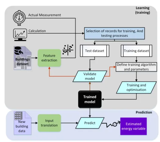
ML models operate as a black box, so further information about the building
207
is not required. The general scheme of supervised learning for modelling building
208
energy is illustrated in Figure 1. As seen, the first step is to select a set of
209
features for representing the building energy system. Although data-driven
210
methods build models with fewer variables than engineering techniques, it is
211
crucial to generate a logical input set for the ML model. These features are not
212
necessarily raw building characteristics or weather data; instead, they could be
213
complex variables calculated from basic ones, e.g. wall to floor ratio and mean
214
daily global radiation (Zhao & Magoul`es, 2012b).
215
Figure 1: General schematic diagram of supervised learning.
The next key stage in utilising MLs is optimisation of model itself. This
procedure which is called tuning plays an important role in the performance
217
of an ML model especially when it is a complex one. Choosing inappropriate
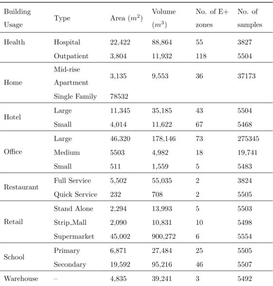
218
hyper-parameters will result in poor accuracy which may falsely be translated
219
as the model failure. Although selecting the right input variables is essential
220
for training a successful machine, the full advantage cannot be taken of ML
221
without tuning the model for that specific training data. Each ML has different
222
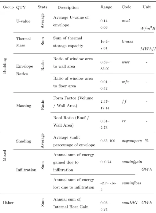
hyper-parameters which govern the learning process. A key point in tuning
223
an ML model parameters is the generalisation. That is to say, how well the
224
learning model applies to specific examples not seen by the model when it was
225
training. Hence, in the procedure of model optimisation, there should be a
226
proper mechanism such as cross-validation to avoid overfitting (i.e. modelling
227
the training data too well).
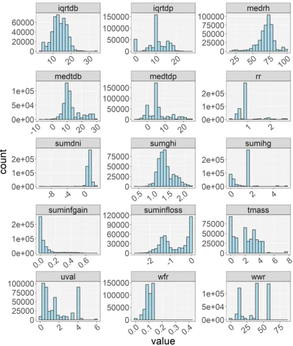
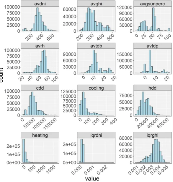
228
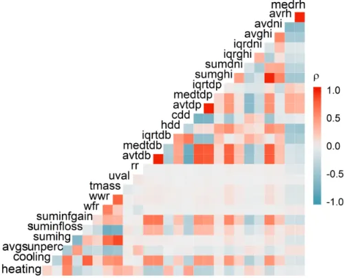
Five ML techniques including ANN, SVM, GP, RF and GBRT are employed
229
to emulate two BPS tools namely EnergyPlus and Ecotect. A standard method
230
that we used to select optimal hyper-parameters is a grid-search combined with
231
k-fold cross-validation. In this procedure, the data is divided intok exclusive
232
subsets, and each combination of model parameters and architecture is fitted to
233
each distinct group ofk−1 subsets and tested on the remaining subset. This
234
process provides a distribution of errors for a given model choice on different
235
parts of the dataset, i.e., an estimate of the general applicability of the model
236
to represent the variation in the dataset. Furthermore, different normalisations
237
such as standard, min-max and robust are applied to data before training
pro-238
cedure. Robust scaler eliminates the median and normalises data according to
239
the inter-quartile range.
240
Basics of each model and the parameters going under optimisation are
ex-241
plained as followings.
242
3.1. Artificial Neural Network
243
Neural networks have been broadly utilised for building energy estimation
244
and known as the major ML techniques in this area. They have been successfully
245
used for modelling non-linear problems and complex systems. By applying
different techniques, ANNs have the capability to be immune to the fault and
247
noise (Tso & Yau, 2007) while learning key patterns of building systems.
248
The main idea of ANN is obtained from the neurobiological field. Several
249
kinds of ANN have been proposed for different applications including, Feed
250
Forward Network (FFN), Radial Basis Function Network (RBFN) and recurrent
251
networks (RNN). Each ANN consists of multi-layers (minimum two layers) of
252
neurons and activation functions that form the connections between neurons.
253
Some frequently used functions are linear, sigmoid ad hard limit functions (Park
254
& Lek, 2016).
255
In FFN which was the first NN model as well as the simplest one, there are
256
no cycles from input to output neurons and the pieces of information moves in
257
one direction in the network. Figure 2 illustrates the general structure of FFN
258
with input, output and one hidden layer.
259
Figure 2: Conceptual structure of feed forward neural network with three layers.
RNN uses its internal memory to learn from preceding experiences by
allow-260
ing loops from output to input nodes. RNN is proposed in various architectures
261
including fully connected, recursive, long short-term memory, etc. This type
of neural network has usually been employed to solve very deep learning tasks
263
such as multivariate time-series prognostication; often more than 1000 layers
264
are needed (Ghiassi et al., 2005).
265
In RBFM, a radial basic function is used as activation function providing
266
a linear combination of inputs and neuron parameters as output. This type of
267
network is very effective for time series estimation (Harpham & Dawson, 2006;
268
Leung et al., 2001; Park et al., 1998).
269
Due to the nature of the datasets, a multilayer perception FFN is utilised in
270
this work. The ANN hyper-parameters which go under optimisation are:
271
• Optimiser: the function that updates the weights and bias;
272
• Activation: a non-linear transformation function which is applied over
273
the input, and then the output is fed to the subsequent layer neurons as
274
input. An ANN without activation function will act as a linear regressor
275
and may fail to model complex systems;
276
• Initialisation: the initial values of weights before the optimiser is applied
277
for training;
278
• Epoch: the number of forward and backward passes for all samples of
279
data;
280
• Batch size: specifies the number of samples that are propagated through
281
the ANN training (i.e. the number of samples in one epoch);
282
• Dropout rate: dropout is a regularisation method for preventing ANN
283
from overfitting and creating more generalised model by randomly
reject-284
ing some neurons during training. Droput rate determines the percentage
285
of randomly input exclusion at each layer;
286
• Size: number of neurons in each layer and number of layers.
287
3.2. Support Vector Machine
288
SVMs are highly robust models for solving non-linear problems and used in
289
research and industry for regression and classification purposes. As SVMs can
be trained with few numbers of data samples, they could be right solutions for
291
modelling study cases with no recorded historical data. Furthermore, SVMs
292
are based on the Structural Risk Minimisation (SRM) principle that seeks to
293
minimise an upper bound of generalisation error consisting of the sum of
train-294
ing error and a confidence level. SVMs with kernel function acts as a two-layer
295
ANN, but the number of hyper-parameters is fewer than that. Another
advan-296
tage of SVM over other ML models is uniqueness and globally optimality of
297
the generated solution, as it does not require non-linear optimisation with the
298
risk of sucking in a local minimum limit. One main drawback of SVM is the
299
computation time, which has the order almost equal to the cube of problem
300
samples.
301
Suppose every input parameter comprises a vector Xi (i denotes the ith
302
input component sample), and a corresponding output vector Yi that can be
303
building heating loads, rating or energy consumption. SVM relates inputs to
304
output parameters using the following equation:
305
Y =W·φ(X) +b (1)
where φ(X) function non-linearly maps X to a higher dimensional feature
306
space. The bias, b, is dependent of selected kernel function (e.g. b can be
307
equal to zero for Gaussian RBF).W is the weight vector and approximated by
308
empirical risk function as:
309 M inimise: 1 2kWk 2+C1 1 N X i=1 Lε(Yi, f(Xi)) (2) Lε isε-intensity loss function and defined as
310 Lε(Yi, f(Xi)) = |f(x)−Yi| −ε, |f(x)−Yi| ≥ε 0, otherwise (3)
Hereεdenotes the domain ofε-insensitivity andN is the number of training
311
samples. The loss becomes zero when the predicted value drops within the band
312
area and gets the difference value between the predicted and radius ε of the
domain, in case the expected point falls out of that region. The regularised
314
constantC presents the error penalty, which is defined by the user.
315
SVM rejects the training samples with errors less than the predeterminedε.
316
By acquisition slack variablesξandξ∗
i for calculation of the distance from the
317
band are, equation (3) can be expressed as:
318 M inmise: ξ,ξ∗ i,W,b 1 2kWk 2+C 1 N N X i=1 ξ+ξi∗ (4) subject to 319 Yi−W·φ(xi)−b≤ε+ξ W·φ(xi) +b−Yi ≤ε+ξi∗ ξ≥0, ξi∗≥0 (5)
The SVM problem using a kernel function ofK(Xi, Xj) (αi, α∗i as Lagrange
320
multipliers) can be simplified as:
321 M aximise: {αi},{α∗i} −ε N X i=1 (α∗i +αi) + N X i=1 Yi(α∗i −αi)− 1 2sum N i=1 N X j=1 (α∗i −αi)(αj∗−αj)K(Xi, Xj) (6) subject to 322 N X i=1 (α∗i −αi) = 0, 0≤αi, α∗i ≥C (7) As mentioned before the number of parameters in SVM with a Gaussian
323
RBF kernel is few as two which areC and Gamma.
324
3.3. Gaussian Process
325
The main drawback of GP modelling is expensive computational cost,
es-326
pecially with the increase of training samples. This is due to the fact that GP
constructs a model by determining the structure of a covariance matrix
com-328
posed ofN×N input variable where the matrix inversion required in predictions
329
has a complexity ofO(N3)
330
Given a set ofnindependent input vectorXj(j= 1,· · · , n), the
correspond-331
ing observations ofyi (i= 1,· · ·, n) are correlated using covariance functionK
332
with normal distribution equal to (Li et al., 2014):
333 P(y;m;k) = 1 (2π)n/2|K(X, X)|1/2 ×exp −1 2(y−m) TK(X, X)−1(y−m) (8) The covariance or kernel function can be derived as
334 K= k(x1, x1) k(x1, x2) · · · k(x1, xn) k(x2, x1) k(x2, x2) · · · k(x2, xn) .. . ... . .. ... k(xn, x1) k(xn, x2) · · · k(xn, xn) (9)
A white noise, σ, is presumed in order to consider the uncertainty. It is
335
assumed that the samples are corrupted (lets suppose as new inputs asx∗) by
336
this noise. In this case covariance ofy is expressed as
337
cov(y) =K(X, X) +σ2 (10)
Theny∗ can be estimated as below.
338 y∗= n X i=1 αik(xi, x∗) (11) αi = K(X, X) +σ2I −1 yi (12)
For GP model three parameters are tuned: kernel, alpha (α) which is the
339
value added to the diagonal of the kernel matrix (equation 11) and the number
340
of restarts of the optimiser for discovering the parameters maximising the
marginal probability. Two combinations of white noise with RBF and Matern
342
covariance functions are used for GP model kernel. Matern kernel is denied as:
343 K(X, X0) = 261−v Γ(v) √ 2v|x−x0| I !v Kv √ 2v|x−x0| I ! (13) Here, Γ is the Gamma function andKv is the modified Bessel function the
344
second-orderv (Owen et al., 1965).
345
3.4. Random Forest
346
Random forest is a collection (ensemble) of randomised decision trees (DTs)
347
(Tin Kam Ho, 1995). DT is a non-parametric ML that establishes a model
348
in the form of a tree structure. DT repeatedly divides the given records into
349
smaller and smaller subsets until only one record remains in the subset. The
350
inner and final sets are known as nodes and leaf nodes. As the precision of DT
351
is substantially subject to the distribution of records on in the learning dataset,
352
it is considered as an unstable method (i.e. tiny alteration in the observations
353
will change the entire structure). To overcome this issue a set of DTs and
354
uses the average predicted values of all independent trees as the final target. In
355
general, RF applies bagging to combine separate models but with sore of similar
356
information and generate a linear combination from many independent trees.
357
RF requires few number of hyper-parameters to be set. The main parameter
358
is the number of independent trees in the forest. There is a trade-off between
359
the accuracy of model and training/prediction computational cost. Thereby,
360
this parameter should be tuned to choose the optimal value. Other
parame-361
ters include the number of features to consider when seeking for the best split,
362
whether bootstrap samples are used when creating trees and minimum number
363
of data sample to split a node and required in each node.
364
3.5. Gradient Boosted Regression Trees
365
Like RF, GBRT is an ensemble of other prediction models such as DTs. The
366
principal difference between GBRT and RF is that the latter one is based on fully
367
developed DTs with low bias and high variance, while the former employs weak
learners (small trees) having high bias and low variance (Breiman, 2017). In
369
GBRT, trees are not independent of each other; instead, each branch is created
370
based on former simple models through a weighting procedure. This approach
371
is known as boosting algorithm. At each inner node (i.e. the split point) given
372
dataset is divided into two samples. Let’s assume a GBRT with three nodes
373
trees; then there will be one split point in which the best segmentation of the
374
data is decided, and the divergence of the obtained values (from the individual
375
averages) are calculated. By fitting on these residuals, the subsequent DT will
376
seek for another division of data to reduce the error variance.
377
Most important parameters for optimising GBRT comprise learning rate
378
(also known as shrinkage) which is a weighting procedure to prevent overfitting
379
by controlling the contribution of each tree, number of trees, maximum depth
380
of tree and the number of features for searching best division, and the minimum
381
number of data sample to split a node and required in each node. Moreover,
382
the sub-sample parameter defines the fraction of observation to be selected for
383
each tree.
384
Rather than conventional GBRT model the recently improved version known
385
as eXtreme Gradient Boosting (XGBoost) algorithm (Chen & Guestrin, 2016)
386
is also evaluated with similar parameters, but some differences. The minimum
387
sum of instance weight controls the generalisation similar to minimum sample
388
split in GBRT. The portion of columns when constructing each tree (colsample
389
bytree) similar to maximum features.
390
3.6. Performance Evaluation
391
Various measurements based on actual and predicted results are calculated,
392
in order to evaluate the performance or accuracy of data-driven models. These
393
include Coefficient of Variance (CV), Mean Bias Error (MBE), Mean Squared
394
Error (MSE), Root Mean Squared Error (RMSE), Mean Squared Percentage
395
error (MSPE), Mean Absolute Percentage Error (MAPE) and MAE (mean
ab-396
solute error). CV is the variation of overall prediction error concerning actual
397
mean values. MBE is used to determine the amount over/underestimation of
predictions. MSE and MSPE is a good inductor of estimation quality. MAE
399
determines the average value of the errors in a set of forecasts and MAPE is the
400
percentage of error per prediction. RMSE has the same unit of actual
measure-401
ments. In this work, RMSE, MAE andcoefficient of determination (R2)
402
are used to present the accuracy of ML models. R2 is the percentage variance
403
in the dependent variable explained by the independent ones. These values are
404 calculated as follows: 405 RM SE= r 1 N X (yi−y)ˆ 2 (14) M AE= 1 N X |yi−yˆ| (15) R2= P(ˆy i−y)¯ 2 P (yi−y)¯ 2 (16) Here, y, ˆy and ¯y represent the real, estimated and average response values,
406
respectively.
407
4. Selected Datasets for Case Study
408
Two building datasets simulated using BPS tools are utilised. First data
409
contains 768 variations of a residential building obtained altering eight basic
410
envelope characteristic (Tsanas & Xifara, 2012), and the second dataset includes
411
various building type represented by 28 envelope and climate features (Rastogi,
412
2016). Each set and the distribution of variables are presented in this section.
413
The prediction targets for both sets are heating and cooling loads.
414
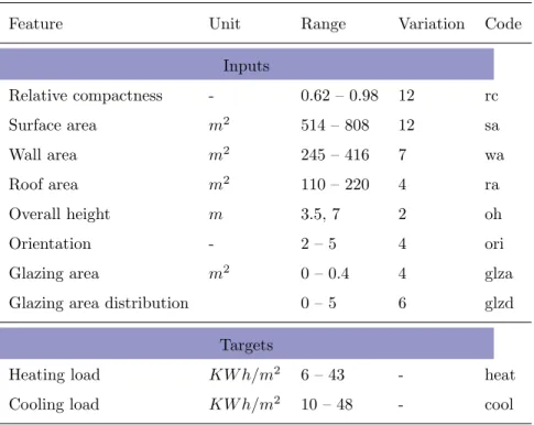
4.1. Ecotect Dataset
415
This dataset was developed by Tsanas & Xifara (2012) and obtained from
416
UCI machine learning repository (Xifara & Tsanas, 2012). It includes 12
resi-417
dential buildings types with the same volume (771.75m3) and varying envelope
418
features, outlined in Table 1. The materials were chosen to achieve the lowest
U-values based on availability in the market (walls: 1.78m2K/W, floors: 0.86,
420
roofs: 0.50 and windows: 2.26). The window-to-floor ratio is varied from 0%
421
to 40%. The glazing distribution on each faade has 6 variants: (0) uniform,
422
with 25% glazing on each side; (1) 55% glazing on the north faade and 15%
423
on the rest; (2) 55% glazing on the east faade and 15% on the rest; (3) 55%
424
glazing on the south faade and 15% on the rest; (4) 55% glazing on the west
425
faade and 15% on the rest; and, (5) no glazing. All combinations were
simu-426
lated using Ecotect with weather data from Athens, Greece, and occupancy by
427
seven people conducting mostly sedentary activities. The ventilation was run in
428
a mixed mode with 95% efficiency and thermostat setpoint range of 19-24◦C.
429
The operating hours were set to 3 pm - 8 pm (15:00-20:00) for weekdays and
430
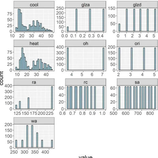
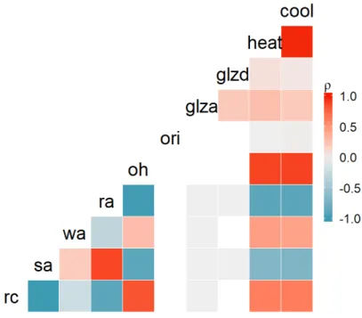
10 am - 3 pm (10:00-15:00) for weekends. The lighting level was set to 300 lx.
431
Figure 3 illustrates the frequency distribution of features and the correlation
432
between each pair of input and target variables is plotted as a heat map matrix
433
in Figure 4.
434
Figure 3 illustrates the frequency of features as histogram graphs. The
435
correlation between each pair of input and target variables is demonstrated
436
using heatmap matrix in Figure 4.
437
4.2. EnergyPlus Dataset
438
This datasets consists of commercial and residential buildings and is
de-439
scribed by Rastogi (2016). The original commercial building models were
down-440
loaded from the US Department of Energy (USDOE) commercial reference
441
building models (DOE). The commercial buildings set includes sixteen types
442
of buildings classified into eight overall groups based on usage. Table 2 presents
443
the building types which are considered in the simulations and the frequency
444
of each with unique features. For each subtype, there are three variations for
445
envelope construction: pre-1980, post-1980, and new construction. Each usage
446
type has the same form, area and operation schedules. The residential
build-447
ings are described by Chinazzo et al. (2015). Variation in the outputs is also
448
introduced by considering several years of historical weather data from many
Table 1: List of features that represent the characteristics of residential buildings for prediction of energy loads
Feature Unit Range Variation Code
Inputs Relative compactness - 0.62 – 0.98 12 rc Surface area m2 514 – 808 12 sa Wall area m2 245 – 416 7 wa Roof area m2 110 – 220 4 ra Overall height m 3.5, 7 2 oh Orientation - 2 – 5 4 ori
Glazing area m2 0 – 0.4 4 glza
Glazing area distribution 0 – 5 6 glzd
Targets
Heating load KW h/m2 6 – 43 - heat
climates (weather stations) and augmenting this data with synthetic weather
450
generated for some climates (Rastogi, 2016).
451
We use the same regression inputs as originally proposed in (Rastogi &
An-452
dersen, 2016). They describe the feature selection as being based on correlation
453
estimation and Principal Component Analysis (PCA). There are three kinds
454
of input variables: climate, building, or mixed. The climate variables were
ex-455
tracted from one year of weather data only and are independent of the buildings
456
simulated. The building features are related to the physical characteristics of
457
the building envelope and independent of the climate. These inputs were
cho-458
sen on the basis of impact on the heating and cooling loads and calculated from
459
geometry, material and structure properties. The mixed parameters represent
460
the interactions between weather and buildings. An input that does not belong
461
to any of these categories, the internal heat gain, was also included to represent
462
the impact of human behaviour. Figure 5 and Figure 6 illustrate the frequency
463
of features and correlation heat-map matrix respectively.
464
Figure 5 illustrates the frequency of features as histogram graphs for
Ener-465
gyPlus Dataset. It can be seen that the each variable is relatively distributed
466
over the possible predefined values. The correlation heat-map matrix presented
467
in Figure 6 shows the in dependency of different features especially building
468
physics related ones from each other.
469
5. Result and Discussions
470
All models are implemented using Python programming language and test
471
have been carried out on a PC with Intel Core i7-6700 3.4GHz CPU, 32GB
472
RAM.
473
The stated goal of this paper is to highlight the importance of tuning
nonlin-474
ear regression models (ML models) to achieve the best predictive performance
475
for a given use case. To put our work in context, it is worth noting the results
476
from the original studies that introduced the datasets used in this paper (Tsanas
477
& Xifara, 2012; Rastogi et al., 2017). Tsanas & Xifara (2012) reported RMSEs of
Table 2: Frequency and size of building types in EnergyPlus data
Building
Usage Type Area (m
2) Volume (m3) No. of E+ zones No. of samples Health Hospital 22,422 88,864 55 3827 Outpatient 3,804 11,932 118 5504 Home Mid-rise Apartment 3,135 9,553 36 37173 Single Family 78532 Hotel Large 11,345 35,185 43 5504 Small 4,014 11,622 67 5468 Office Large 46,320 178,146 73 275345 Medium 5503 4,982 18 19,741 Small 511 1,559 5 5483
Restaurant Full Service 5,502 55,035 2 3824
Quick Service 232 708 2 5505 Retail Stand Alone 2,294 13,993 5 5503 Strip Mall 2,090 10,831 10 5498 Supermarket 45,002 900,272 6 5554 School Primary 6,871 27,484 25 5505 Secondary 19,592 95,216 46 5507 Warehouse – 4,835 39,241 3 5492
Table 3: List of EnrgyPlus features extracted for model training
Group QTY Stats Description Range Code Unit
Building U-value Av erage Average U-value of envelope 0.14– 6.06 uval W/m2K Thermal Mass Sum Sum of thermal storage capacity 1e-4– 7.61 tmass M W h/K Envelope Ratios Ratio
Ratio of window area to wall area
0.58– 85.00
wwr
-Ratio of window area to floor area 0.01– 0.42 wf r -Massing Ratio
Form Factor (Volume / Wall Area)
2.47– 17.14
f f
-Roof Ratio (-Roof / Wall Area) 0.31– 2.73 rr -Mixed Shading Av erage Average sunlit percentage of envelope 0.35–100 avgsunperc % Infiltration Sum
Annual sum of energy gained due to
infiltration
0–0.74 suminfgain GW h Annual sum of energy
lost due to infiltration
-2.7– -1e-4 suminfloss Other Sum Annual sum of Internal Heat Gain
0.03– 5.24
sumIHG GW h
1.014 and 2.567 for heating and cooling loads, respectively. Our best RF model
479
achieved 0.476 and 1.585 for the same variants, a roughly 40% improvement in
List of features extracted for model training (cont.)
GRP QTY Stats Name Range Code Unit
Climate
Degree Days
Sum
Annual sum of cooling degree days (9.6–160)e4 cdd
C-day
Annual sum of heating degree days 424–64878 hdd
Dry Bulb Temp (Hourly)
Avg. Annual average of dry bulb temperature -3.11–28.39 avgtdb
C
Median
Median dry bulb temperature -7.20–30 medtdb
IQR Inter-quartile range of dry bulb Temp 3.6–34 iqrtdb
Dry Point Temp (Hourly)
Avg. Annual average of dry point temperature -7.41–21.43 avgtdp
C
Median
Median dew point temperature -6.4–24.2 medtdp
IQR
Inter-quartile range of dew point
temperature 0–26.8 iqrtdp Global Hori-zontal Irradia-tion (Hourly) Avg.
Annual average of global horizontal
irradiation 190–509 avghi M W h/m 2 Sum
Annual sum of global horizontal
irradiation 0.40–2.23
sumghi
IQR
Inter-quartile range of global horizontal irradiation (0.84–5.2)e-3 iqrghi Direct Normal Irradiation (Hourly) Avg.
Annual average of direct normal
irradiation 57–676 avgdni M W h/m 2
Sum Annual sum of direct normal irradiation -10.34–3.15 sumdni
IQR
Inter-quartile range of direct normal irradiation (0.38– 26.3)e-4 iqrdni Humidity (Hourly)
Avg. Annual average of relative humidity 22–98 avrh %
Median
accuracy in term of RMSE (kWh/m2). Rastogi et al. (2017) report an error of
481
10-15 kWh/m2 on the EnergyPlus dataset while we achieve 6-10 kWh/m2.
Ta-482
bles 5 and 6 give an overview of results for the Ecotect and EnergyPlus datasets,
483
respectively. The tables contain Coefficients of Determination (R2), Root Mean
484
Square Errors (RMSE), Mean Absolute Errors (MAE), fit time, test time, and
485
number of parameters for the best combination of hyper-parameters; the
av-486
erage fitting time of all tested models; and the total number of iterations for
487
comparison of time complexity. Here, the test time is the average of predictions
488
of all folds (192 data points per fold for Ecotect and 1,000 for Energy Plus). For
489
EnergyPlus data, GP is excluded from the comparison because the training time
490
is extremely high for large datasets. Most ML models are capable of forecasting
491
multiple outputs at the same time. However, we tuned all models separately for
492
heating and cooling loads. None of the techniques obtained the best accuracies
493
for both target values using the same combination of hyper-parameters. This
494
inconsistency indicates that the importance of input variables as well as the
cor-495
responding weights are different. Hence, two independent models are required,
496
rather than training a single model.
497
Though the datasets are drawn from different simulators, similarities in the
498
performance of the models do emerge. The lowest RMSE for both heating
499
and cooling loads is achieved by XGBoost, followed by GBRT and RF. These
500
models are all based on decision trees, but unlike RF the other two do not
501
build independent trees. Hence, they train models slightly faster than RF.
502
Considering prediction time in addition to accuracy, however, GBRT is slightly
503
faster than XGBoost but has comparable accuracy. The NN models tend to
504
have the fastest prediction times, which might make them more appropriate for
505
applications requiring very large numbers of simulation estimates. For example,
506
optimising many building parameters, each with several possible choices, under
507
a sample of uncertain operating conditions, such as the problem described in
508
(Rastogi et al., 2017). We find that GP is the slowest and least accurate model.
509
This is partially due to the challenge of using large datasets with GP regression;
510
since the time complexity of GP isO(N3) (whereNis the number of data points
T able 5: Result of tuning ML mo del for Ecotect sim ulated dataset. SVM RF NN GP GBR T X GBo ost Heat Co ol Heat Co ol Heat Co ol Heat Co ol Heat Co ol He at Co ol R 2 0.996 0.972 0.998 0.973 0.997 0968 0.981 0.944 0.999 0.995 0.999 0.998 RMSE 0.475 1.622 0.476 1.585 0.491 1.711 1.381 2.279 0.366 0.677 0.300 0.401 MAE 0.654 1.082 0.332 0.98 0.369 1.120 0.852 1.579 0.254 0.486 0.189 0.294 Fit time (s) 2.19 21.09 0.75 0.73 0.106 0.131 18.86 24.63 0.499 0.655 0.326 0.585 Mean fit time (s) 323.77 177.28 0.72 0.75 1.23 0. 9 9 17. 0 0 18. 65 0. 20 0. 19 0 .28 0.28 T est time 0.005 0.005 0.090 0.104 0.001 0.001 0.019 0.018 0.021 0.031 0.045 0.107 Num b er of parameters 2 3 7 3 7 6 T otal iteration 21 36 3240 30 3456 2160
T able 6: Result of tuning ML mo del for 5000 records of EnergyPlus dataset. SVM RF NN GBR T X GBo ost Heat Co ol Heat Co ol Heat Co ol Heat Co ol Heat Co o l R 2 0.965 0.973 0.973 0.968 0.966 0969 0.980 0.986 0.982 0.986 RMSE 14.318 8.763 12.720 9.400 14.068 9.376 10.721 6.296 10.386 6.270 MAE 5.622 3.465 5.057 4.841 7.472 4.932 4.400 3.365 4.130 3.143 Fit time (s) 177.66 406.31 6.35 34.873 126.29 10.88 6.363 1.789 4.897 4.871 Mean fit time (s) 1641.91 1197.16 17.6 19.54 21.32 17.19 4.85 4.92 4.61 4.55 T est time 0.483 0.507 0.333 0.595 0.008 0.010 0.244 0.078 0.228 0.219 Num b er of parameters 2 3 7 3 7 T otal iteration 21 36 3240 3456 2160
used for training/fitting), the training speed is not comparable with other ML
512
models and inversion of matrices of size{N, N}is unfeasible for largeN. Thus,
513
studies using GP have used small datasets, usually less than a few thousand
514
(Heo et al., 2012; Zhang et al., 2013; Noh & Rajagopal, 2013; Rastogi et al.,
515
2017; Burkhart et al., 2014; Zhang et al., 2015). However, since GP regression
516
allows for the automatic estimation of prediction uncertainty, it is useful in
517
some cases. An example is the estimation of summary statistics, where it is
518
more informative to know the uncertainty of, e.g., annual heating and cooling
519
loads, rather than just a point estimate. Although all models predict the energy
520
loads with high accuracy, the use case should determine the most appropriate
521
model. For example, increasing the number of records (size of training data), the
522
fitting and forecasting time of SVM rises significantly. The training size of NN
523
is slightly increased as well, but it is still the fastest predictor by a considerable
524
margin (10-20 times faster). GBRT and its variant XGBoost achieve the best
525
RMSE. However, the increased accuracy and sophistication of models like NN
526
and XGBoost comes with the penalty of requiring very large training datasets
527
(e.g., the 25,000 simulations used here). This could be an issue where a model
528
has to trained on the fly, i.e., where simulating 25,000 distinct cases to train
529
an accurate model is prohibitively expensive. As expected, using more data to
530
fit a model increases the predictive accuracy of all models, such that complex
531
models with more parameters lose out to simpler models that have seen more
532
data, provided the simpler models can use the additional data available. In
533
summary, where sufficient training data is available and the testing or use cases
534
are not too dissimilar from the training data, the use of models such as GBRT
535
and NN improves accuracy. Where training data is harder to generate, or a
536
model must be trained on the fly with a small dataset, techniques such as GP
537
provide adequate predictions.
538
5.1. Performance of the Best Model
539
We now discuss the performance characteristics of the best models for each
540
dataset. The results are illustrated using two kinds of plots: predicted
mated) loads (ˆy) against loads from the simulator (y), and the distribution of
542
errors between simulated-predicted pairs (ˆy−y). Figures 9 and 7 show the
543
values predicted by tuned GBRT models against their corresponding simulated
544
heating and cooling loads for the Ecotect and EnergyPlus datasets, respectively.
545
The error distributions of these estimations are given in Figure 10 and 8.
546
(a) (b)
Figure 7: Actual and predicted (a) heating and (b) cooling loads of EnergyPlus dataset.
5.2. Effect of Increasing Size of Training Data
547
Given that using large datasets for training seems to improve the predictive
548
accuracy of all models, we investigated the effect of increasing the size of the
549
training dataset on accuracy. Figure 11 shows RMSE versus size of training
550
dataset for the GBRT model. A 10 fold cross-validation is used to obtain the
551
worst, best and mean RMSE over all folds. Mean training time is also displayed
552
as the top axis to show computational cost. Although the best result is obtained
553
by the highest number of samples tested, 25,000 is enough to build a reliable
554
model considering the fitting time and error gap. At this point, the mean RMSE
555
is equal to 7.770 kWh/m2and time required to fit the model is 66.02 seconds.
556
On the other hand, using 400,000 samples and fitting over 2600 seconds, mean
557
RMSE only goes down to 2.338 kWh/m2 (4% of average heating loads).
(a)
(b)
Figure 8: Error distribution of (a) heating and (b) cooling loads prediction for EnergyPlus dataset.
(a) (b)
Figure 9: Actual and predicted (a) heating and (b) cooling loads of Ecotect dataset using GBRT model.
(a) (b)
Figure 10: Error distribution of (a) heating and (b) cooling loads prediction for Ecotect dataset. The red dashed line is for a theoretical normal PDF with the same parameters.
5.3. Feature Importance and Selection
559
To emphasise the importance of features in predicting different loads, we
560
present a sensitivity analysis using two approaches. First, we present the
fea-561
ture importance calculated by the RF models. RF creates many decision trees
562
and the amount of weighted variance explained by each feature can be
calcu-563
lated for each tree. For a forest, the variance explained by each feature can be
564
averaged and the features ranked according to this measure. Here, we trained
565
30 RF models using 100,000 randomly selected samples to obtain an empirical
566
distribution of feature importance, shown in Figure 12.
567
As the best model (GBRT) doesn’t provide the possibility of analysing
sen-568
sitivity to the input variables in the same way, we used a global variance-based
569
method called the Sobol method Sobol (2001); Saltelli (2002). Unlike RF, GBRT
570
does not generate unique trees. Rather, each trees is correlated to the last. To
571
facilitate a comparison, we fitted 30 different models and used them to evaluate
572
the 150,000 samples generated by the algorithm. The Sobol first-order indices
573
of features is illustrated in Figure 13. We see that the importance of features
574
to this method is less stable in GBRT than RF. However, since it is calculated
575
directly from the original data, it is more representative of the features of the
576
dataset itself.
577
For a final test, we examined the effect of dropping variables that the model
578
does not deem to be important. Based on the results of the Sobol comparison,
579
we identified the following features to drop: ‘avrh’, ‘avdni’, ‘iqrdni’, ‘iqrghi’,
580
‘medrh’, ‘sumdni’ for both loads, and ‘avghi’, ‘sumghi’ for cooling only. All
581
of the dropped variables are climate-related, which implies that there may be
582
too many variables used to explain variance due to climate. The GBRT with
583
fewer features was also trained and tested over 10 folds with 25,000 random
584
samples. The results of training a model with a reduced feature set is compared
585
with using the full set of features in Table 7. We see that removing features to
586
which the model is apparently insensitive does not negatively affect the model
587
performance. However, the time complexity of training model is reduced due to
588
a reduction in the size of the dataset. Given that this result applies only to this
(a)
(b)
Figure 12: Importance of features for (a) heating and (b) cooling loads prediction using RF model.
(a)
(b)
Figure 13: Sobol first-order indices of features in predicting (a) heating and (b) cooling loads using best ML model.
dataset and cannot be generalised to all buildings or EnergyPlus simulations,
590
this is not a repeatable result unless we are confident that the dataset used for
591
training represents the use case or problem completely.
592
Table 7: Performance comparison of ML models with full and reduced feature sets determined by sensitivity analysis.
Heating Load Cooling Load
All inputs
Selected
inputs All inputs
Selected inputs RMSE 7.871 7.648 4.455 4.384 MAE 2.127 2.085 2.314 2.310 R2 0.991 0.991 0.993 9.993 Fit time (s) 61.621 48.420 9.387 7.700 Test time (s) 0.642 0.622 0.151 0.145 6. Conclusion 593
The research presented in this paper addresses the gap in using ML methods
594
for estimating building energy loads through a comprehensive study of common
595
ML models fitting over energy simulation data. As became evident in the
re-596
viewed literature, despite the wide usage of MLs in this field, a conclusion on
597
selecting the right model for the energy prediction was not possible. The main
598
reason is that most of the research works have focused on the first eminent
599
part of statistical modelling which is features selection. This paper discussed
600
the importance of ML model optimisation in providing a fair comparison of
dif-601
ferent methods in term of accuracy, the simplicity of tuning and training and
602
response times of model. This study optimised the hyper-parameters of each
603
model for both heating and cooling loads to obtain the best precision. It was
604
also indicated that when there are two energy indices as cooling and heating
605
loads to be estimated by model, it is desired to optimise and train separate
machines. To that end, the role of ML model in recognising most impacting
607
factor in prediction of building loads. The other key outcome of this research
608
is a set of recommendations for the quick selection of ML model based on the
609
data and usage.
610
The results indicated that the standard and advanced GBRTs provide the
611
most accurate predictions, considering the RMSE value. However, when the
612
data was simple (in term of input variables and size), SVM was proven to be the
613
best choice because of simplicity and the speed of calculations. The results also
614
ascertained that for complex data sets, multi-layer NNs are more appropriate
615
when there is a massive demand for ever-more energy simulations. In this case,
616
NN was proven to be capable of estimating incredibly faster than other MLs
617
methods. It should be noted that NN is complicated, and requires an expert to
618
particularly tune it for each studied case; otherwise, NNs could fail quickly.
619
Comparison of tuned models with previous studies highlighted the
impor-620
tance of determining the hyper-parameters for each data set, and the fact that
621
this can become more crucial by increasing the size and intricacy of the
ex-622
aminations set. By fitting individual models for heating and cooling loads, it
623
was shown that one assorted set of model parameters could not accurately
esti-624
mate both values. Therefore, unlike previous studies, it is recommended by this
625
study to train models for each energy load independently. The other approach
626
would be the implementation of a specific sorting algorithm to find balanced
627
values. As results signified, it is suggested to attain a higher accuracy feeding
628
the machines with more number of instances is essential. It might not be a
629
solution for measured historical data; however further simulation using various
630
values of inputs could be aggregated during the design stage prior to optimising
631
the building. Another identified critical factor was that the features must be
632
thoroughly selected/created for representing building characteristics and needs
633
should be appropriately investigated before developing models.
634
The findings of this study concurred with the seminal literature by
demon-635
strating the fact that MLs techniques are overtly superior over the conventional
636
statistical and engineering methods in building energy calculation. This study
also revealed the further power of those ML methods and newly developed ones
638
when they thoroughly optimised. There are several ready to use software
pack-639
ages (e.g. Matlab) providing various ML models with few parameters to modify.
640
Nevertheless, it is advisable to use simpler models like SVM or RF with an
ad-641
vanced programming language, such as Python and R.
642
Finally, the most important features are recognised using sensitivity analysis
643
methods, and the investigation of the model with reduced dimension revealed
644
that even though the computational cost of building model is reduced, the
645
performance didn’t alter. This analysis demonstrated the capability of MLs
646
in eliminating inessential input parameters, while most statistical methods are
647
susceptible to these type of features.
648
The methods discussed in this work proved the efficiency of ML models in
649
predicting building energy loads as well as performance. The fast and accurate
650
calculation of those values paves pathways for more informed and productive
de-651
sign decisions for built environments. Furthermore, along with the optimisation
652
algorithms, ML seems as a promising solution for efficacious retrofit planning of
653
complex buildings, where engineers are not capable of massive calculations.
654
Appendix A. Detailed Results for Tuning ML Models
655
The detail of tuning each ML model is presented in this section. Some
656
models have several parameters, so the brute force search includes thousands of
657
train-test models. Therefore, it is not possible to present the list of all results
658
in this paper. However,Tables A.8 to A.13 demonstrates the parameters for the
659
best models predicting energy loads of both datasets. In each table the best
660
model is highlighted with light blue colour.
661
In order to reduce the time complexity of tuning ANN model, the number
662
of epochs was fixed at 500 and the other parameters were optimised. Then
663
the optimal number of propagations was separately obtained using the best
664
parameters. As shown in the Figures A.14 (a) and (b)
Table A.8: Detail of optimising SVM for both datasets.
EPlus Data Ecotect Data SVM Parameters
Heat RMSE Cool RMSE Heat RMSE Cool RMSE C
Gamma 14.318 9.785 0.677 1.622 10,000 1 18.988 9.774 0.654 1.667 1000 1 15.720 9.261 0.660 1.756 1,000,000 0.1 15.313 10.302 0.978 1.842 1,000,000 1 21.626 8.763 0.815 2.048 100,000 0.1 31.415 9.452 2.108 2.636 10,000 0.1 43.719 17.833 2.627 3.365 10,000 0.01 60.974 31.658 3.304 3.886 1 0.1 60.974 31.658 3.304 6.550 1 0.01
Table A.9: Detail of optimising RF for both datasets.
EPlus Data Ecotect Data RF Parameters
Heat RMSE Cool RMSE Heat RMSE Cool RMSE Boot-strap Max features No. of es-timators 12.873 9.894 0.568 1.585 False sqrt 600 12.720 9.693 0.576 1.605 False sqrt 400 14.556 10.734 0.604 1.612 True sqrt 200 13.334 10.214 0.502 1.658 False log2 1000 14.551 9.691 0.476 1.683 True auto 600 14.584 9.600 0.478 1.691 True auto 800 24.189 13.727 0.536 1.814 False auto 1000 14.199 10.995 0.616 1.604 True sqrt 400
T able A.10: Detail of optimising GBR T for b oth datasets. EPlus Data Ecotect Data GBR T P arameters Heat RMSE Co ol RMSE Heat RMSE Co ol RMSE Learning rate Max depth max features Min sample leaf Min sample split
No. e s-timator Sub sample 13.157 7.402 0.388 0.677 0.15 8 None 1 100 1500 1 11.534 6.667 0.366 0.893 0.15 3 None 1 2 1500 1 12.914 6.297 0.399 1.033 0.25 3 sqrt 1 2 1500 1 10.721 8.855 0.514 1.261 0.1 8 sqrt 1 2 2000 1 13.257 9.608 0.523 1.578 0.01 13 sqrt 1 2 1250 0.9 17.843 8.654 3.77 3.895 0.01 8 sqrt 200 100 500 1 22.775 9.856 8.732 8.524 0.001 13 sqrt 200 100 1250 0.7 26.221 15.625 10.054 9.725 0.25 3 sqrt 1000 100 1750 1 35.518 21.196 10.003 9.726 0.1 8 sqrt 1000 1000 1000 0.9 46.991 24.279 9.996 9.720 0.1 3 sqrt 1000 2 1000 0.8 49.515 24.542 9.996 9.722 0.1 3 None 1000 100 1500 0.7 21.578 11.642 10.422 9.746 0.15 13 None 500 1000 1000 0.8
T able A.11: Detail of optimising X GBo o st for b oth datasets. EPlus Data Ecotect Data X GBo ost P arameters Heat RMSE Co ol RMSE Heat RMSE Co ol RMSE P ortion of features Learning rate Max depth Min child weigh
t No. estimator Sub sample 10.909 8.145 0.303 0.401 0.6 0.1 8 1 1750 0.9 11.616 9.002 0.300 0.452 0.6 0.1 13 1 750 0.7 12.273 8.048 0.323 0.573 0.38 0.1 8 1 1250 0.8 12.436 8.18 0.329 0.804 0.6 0.01 13 1 1750 1 11.302 6.270 0.413 1.131 0.6 0.1 3 1 2000 0.7 10.387 6.382 0.409 1.115 0.6 0.1 3 3 2000 0.9 13.738 9.982 0.306 0.443 0.5 0.1 13 1 1750 0.8 16.030 12.706 0.337 0.557 0.4 0.5 13 3 1000 0.7 20.003 10.434 0.304 0.433 0.1 0.1 8 1 10000 0.8 23.821 14.138 0.343 0.567 0.1 0.25 13 3 1000 0.7 26.266 16.581 0.365 0.578 0.1 0.5 13 3 1500 0.8 57.263 35.554 9.459 10.412 0.6 0.01 3 1 200 0.7
(a)
(b)
Figure A.14: RMSE of ANN model predicting energy loads for (a) EPlus and (b) Ecotects datasets against number of epochs.