Statistic Software for Neighbor Embedding

(1)

Instructor

Statistic Software for Neighbor Embedding

Zhao Jie

Helsinki May 29, 2017

UNIVERSITY OF HELSINKI Department of Maths and Statistics

(2)

Faculty of Science Department of Maths and Statistics Zhao Jie

Statistic Software for Neighbor Embedding Statistics

May 29, 2017 60

Manifold Learning, Neighbor Embedding, R, Rcpp

Dimension reduction presents expanding importance and prevalence since it lessens the challenge to data visualization and exploratory analysis that numerous science areas rely on. Recently, non-linear dimension reduction (NLDR) methods have achieved superior performance in coping with complicated data manifolds embedded in high dimensional space. However, conventional statistic software for NLDR visualization purpose (e.g Multidimensional Scaling) often gives undesired de-sirable layouts. In this thesis work, to improve the performance of NLDR for data visualization, we study the recently proposed and efficient neighbor embedding (NE) framework and develop its software package in statistic software R. The neighbor embedding framework consists of a wide family of NLDR including stochastic neighbor embedding (SNE), symmetric SNE etc. Yet the original SNE optimization algorithm has several drawbacks. For example, it cannot be extended to other NE objective functions and requires quadratic computation cost. To address these draw-backs, we unify many different NE objective functions through several software layers and adopt a tree-based approach for computation acceleration. The core algorithm is implemented in C++ with an lightweight R wrapper. It thus provides an efficient and convenient package for researchers and engineers who work on statistics. We demonstrate the developed software by visualizing the two-dimensional layouts for several typical datasets in machine learning research including MNIST, COIL-20 and Phonemes etc. The results show that NE methods significantly outperform the tra-ditional MDS visualization tool, indicating NE as a promising and useful dimension reduction tool for data visualization in statistics.

Tekijä — Författare — Author

Työn nimi — Arbetets titel — Title

Oppiaine — Läroämne — Subject

Työn laji — Arbetets art — Level Aika — Datum — Month and year Sivumäärä — Sidoantal — Number of pages

Tiivistelmä — Referat — Abstract

Avainsanat — Nyckelord — Keywords

Säilytyspaikka — Förvaringsställe — Where deposited

(3)

1 Introduction

With the rapid development of data collection techniques, the amount, source and complexity of data receive explosive growth. One of the most thorny issues based on such “big data” is how to extract and to analyze the essence of data escaping from the data redundancy which commonly appears as too-high observation dimensionality. Dimension reduction techniques have thus been drawing increasing interests since they are capable to significantly reduce the difficulty for following research processes in many science domains such as data visualization, exploratory analysis and multi-perceptron training.

Relying on a simple assumption that, data points in high dimensional space exactly or approximately lie on a lower dimensional manifold embedded in the high dimen-sional space, a series of dimension reduction methods have been proposed. Principal Component Analysis (PCA) [Hot33] considers a linear or approximate linear global manifold and project the high dimensional data points to the axes that will max-imize the variance. For its simplicity and efficiency, PCA is regarded as the most popular dimension reduction method in decades. However, restricted by its linear nature, PCA does not perform well in coping with the complicated high dimensional manifold [vdM09]. To overcome this drawback, novel algorithms were proposed from a non-linear view, not the same as PCA with linear matrix transformation and pro-jection.

Multidimensional Scaling (MDS) [Tor52], which attempts to preserve the distances in high dimensional space, allocates the low dimensional coordinates to minimize the difference between the pairwise distances in both high and low dimensional space. Sammon mapping [Sam69] adds higher weights on closer pairwise data points based on the MDS cost function. Isomap [TDSL00] makes further improvement to retain the manifold by replacing the direct Euclidean distance in MDS with the geodesic distance after importing the k nearest neighbor graph to represent the manifold. Local Linear Embedding (LLE) [RS00] develops a coordinate-free route to seek the best matching of high and low configurations, based on the weighted “neighborhood”. Other methods like Maximum Variance Unfolding (MVU) [WS06], Self-Organizing Map (SOM) [Koh98], Laplacian Eigenmap (LE) [BN01] and so on all illustrate insightful comprehension on dimension reduction.

Meanwhile, conventional non-linear dimension reduction methods have one or more drawbacks. For instance, MDS and Sammon mapping are expensive to optimize and

(6)

easily getting stuck at poor local optima; LLE encounters the collapse problem and it’s cumbersome to deal with the outliers [LV07].

Later Hinton and Roweis proposed a non-linear dimension reduction method, Stochas-tic Neighbor Embedding(SNE) [HR02], to produce a better dimension reduction performance. It soon receives great popularity since it outperforms most of the di-mension reduction approaches with plenty of following variants including Symmetric SNE, Student t-distributed SNE [vdMH08] and weight symmetric SNE [YPK14] etc. We study the NE framework and focus on weighted t-SNE which has not been further discussed to evaluate its performance in data visualization. Meanwhile, current conventional non-linear dimension reduction and visualization software tools can not provide satisfying results. For us, it will be meaningful to develop an NE package in statistic software, R, to achieve the scalability, efficiency and simplicity of NLDR implementation. Conventional MDS algorithms are taken as the counterpart of NE for the performance comparison, not only because of its popularity, but also for Hinton’s interpretation of SNE as a probabilistic version of local MDS. Multiple typical datasets in machine learning are utilized for the result evaluation. The corresponding results clearly demonstrate the advantages of the proposed method and software.

This thesis is outlined as follows. We review the NE framework and critical details in Section 2. The optimization techniques are discussed in Section.3, following a time line of its development. Section.4 explains the algorithm implementation in R covering both R and C++ level. Section.5 introduces the datasets used in experiment and illustrates the results visualization of NE and MDS. Conclusion and discussion for future work are contained in Section 6.

2 Neighbor Embedding

In this section, we make a detailed introduction to neighbor embedding (NE) method starting from presenting the most prevalent non-linear dimension reduction method, MDS in Section 2.1. The framework of the original stochastic neighbor embedding (SNE) method is introduced in Section 2.2. Later parts cover multiple components managing to improve the performance of NE methods. Section 2.3 discusses the techniques to characterize the high dimensional probabilities. Divergences and low dimensional probabilities are introduced in Section 2.3 and 2.4 respectively.

(7)

2.1 Multidimensional Scaling

Multidimensional Scaling (MDS) is a popular dimension reduction technique which takes proximity data as input, containing the information of dissimilarities between high dimensional pairwise data points. Conventionally, the proximity or dissimilarity is expressed as distance of which the selection may form multiple variants of the MDS method.

In general, MDS attempts to achieve a goal that, given the high dimensional data points X ={x1,x2,· · · ,xN} ∈Rk, obtain the mapped (configuration, embedding) points y1,y2,· · · ,yN in low dimensional space Rd that would optimally maintain high dimensional dissimilarities.

The original or the classical MDS was proposed by Togerson [Tor52]. Meanwhile, classical MDS has a more complicated cost function namedStrain based on the inner products of low dimensional mappingshyi, yjiand requires a two-step transformation process to utilize the information. Kruskal in 1964 developed the leading MDS algorithm, a non-metric MDS [Kru64] which has a more trivial interpretation. The main gap between these two methods is the setting of cost function. The leading MDS has a cost function called Stress with the form

E =StressD(y1,y2,· · · ,yN) = X i X j (dist(xi,xj)− kyi−yjk)2

where dist(xi,xj) is commonly picked as a monotonic function to describe the high dimensional dissimilarity. The dimension d for the low dimensional space is usually set to d= 2 or d= 3 in order to operate the data visualization.

MDS variants can be divided into two subsets by either the high dimensional dissim-ilarity measure or the low dimensional mapping description. For high dimensional pairwise data pointsxi and xj, the dissimilarity can be metric or non-metric, where for instance non-metirc applies the ranks. Meanwhile, low dimensional mapping may take the Togerson inner products or Kruskal distance as a low dimensional dis-tance measure. Buja et al. discussed further for the topic and gave the more general forms of both metric and non-metric families including the power transformation for metric MDS and isotonic transformation for the non-metric [BSL+08].

Although MDS overall produces popular output, it still has flaws. Two main types are that (1) close data points in high dimensional space are mapped far apart in low dimension, (2) dissimilar, far apart high dimensional data points are put closely

(8)

in low dimension. Venna and Kaski defined these phenomenons as trustworthy and continuity [VK06]. For MDS, multiple variants have been proposed to overcome or reduce these mismatch.

Venna and Kaski proposed local MDS [VK06], which is inspired by another MDS variant, curvilinear component analysis (CCA) [DH97], to improve the MDS perfor-mance by seeking a balance between trustworthy and continuity. The cost function of local MDS is as follows E =1 2[(1−λ)(d(xi,xj)−d(yi,yj)) 2_F₍_d_(y i,yj), σi) +λ(d(xi,xj)−d(yi,yj))2F(d(xi,xj), σi)] , (1) where F(d(yi,yj), σi) = ( 1 if d(yi,yj)≤σi 0 if d(yi,yj)> σi .

Coefficient F represents the the influence zone of one data point in the low dimen-sional space whileσi would be adjusted for a certain containment. Parameter λcan be tuned to achieve the optimal tradeoff between trustworthy and continuity. The two parts of the cost function penalize the two kinds of mismatch respectively in order to obtain a global balance of attraction and repulsion among the data points. This reveals a significant similarity with NE framework.

In addition to mismatching, the optimization process also annoys the MDS users. Classical and distance MDS just implement the simple straightforward gradient de-scent methods to minimize the cost function which usually leads to a poor local optima. A plenty of improvements were developed including random initialization of output coordinates and stochastic gradient descent technique. Klock and Buh-mann modified the annealing approach for the optimization task and receive satis-fying result [KB00]. Such efforts just indicate the critical role for the optimization techniques in dimension reduction practical work.

2.2 NE framework

Stochastic Neighbor Embedding (SNE), which applies the neighborhood among high dimensional data points and emphasizes the local structure preservation, broadens a new horizon for the dimension reduction techniques. A general comprehension of NE is optimizing a divergence between neighborhoods in the input and output spaces.

(9)

In the original SNE algorithm, different from MDS using distance functions to eval-uate the pairwise data points similarity, a conditional probability is chosen to assess the probabilistic similarity between xi and xj meaning that conditional on pointxi, how probable the point xj will be chosen as xi’s neighbor representing the neigh-borhood relation.

The conditional probability for high dimensional data pointxi pickingxj as neighbor has the form of

pj|i = exp(−kxi−xjk2/2σ2i) P k6=iexp(−kxi−xkk2/2σi2) and pi|i = 0.

SNE considers that the conditional neighborhood probabilities have already pro-vided sufficient information to capture the embedded manifold in high dimensional space. With the construction of high dimensional probabilities, the corresponding low dimensional probabilities have an analogous form that

qj|i = exp(−kyi−yjk2) P i6=kexp(−kyi−ykk2) and again qi|i = 0,

where yi and yj are the mapped points of xi and xj respectively.

Now suppose that if the relation betweenxiandxj in high dimensional space is well-preserved in low dimensional space byyi andyj, then the difference betweenpj|i and

qj|i should be infinitesimal. SNE takes advantage of Kullback-Leibler divergence as the criterion to evaluate the goodness of preserving such relation and manifold. The cost function of SNE is

C =X i KL(PikQi) = X i X j pj|ilog pj|i qj|i

in which Pi denotes all the conditional probabilities given data point xi and Qi denotes the corresponding probabilities given yi in low dimensional space. In the other word, for everypj|i, SNE attempts to find aqj|ias close as possible respectively. Since the cost function developed from Kullback-Leibler divergence is asymmetric, trustworthy and continuity defined in Section 2.1 are not equally preferred. In SNE, trustworthy that close data points in high dimensional space are mapped far apart will cause a high cost while continuity only brings a comparably very small cost

(10)

due to the log term in the cost function. This indicates that SNE focuses more on preserving the local structure of the manifold embedded in the high-D space. SNE implements straightforward gradient descent method to minimize the cost func-tion where the gradient has a form of

δC δyi

= 2X j

(pj|i−qj|i+pi|j −qi|j)(yi−yj).

This gradient has a trivial physical interpretation as the composition of forces among data points [HR02]. The interaction between pairwise data points can be simulated by a spring giving a force as either attraction or repulsion depending on spring extension which is yi −yj. Simultaneously, pj|i −qj|i +pi|j − qi|j determines the stiffness of the spring. If p > q, points yi and yj will be attracted together. On the contrary,p < q indicates that yi and yj will be repelled further.

As the earliest version in NE algorithm, SNE outperforms almost all the conventional dimension reduction techniques. However, SNE still exposes several drawbacks such as complexity in optimization and crowding problem in output. A series of vari-ants inspired by SNE have been proposed with modification on different portions of SNE framework like the selection of low-D probabilities and further divergence exploration.

2.3 Similarity

NE methods replace distance functions with probabilities to represent the similari-ties among high-D data points and low-D mapped points. The original SNE chooses a Gaussian distribution for both pj|i and qj|i calculated by the exact value of vector elements for vectorial data form. However, such Gaussian kernel yields huge com-putation expense due to the exponential term especially when the size of dataset is large. In fact, suppose two points i and j are excessively far apart in high-D space, the probability for i and j being neighbors will be extremely small meaning that evaluating every pairwise relations of high-D data points is not essential. Only the points satisfying a threshold of “neighborhood” will be taken into the considera-tion for similarity calculaconsidera-tion. This scheme is achieved by constructing a k nearest neighbor graph to significantly simplify the computation.

(11)

2.3.1 k Nearest Neighbor Graph

k-Nearest Neighbor Graph(kNNG) [PS12] is developed from the classicalk-Nearest Neighbor algorithm by adding a process of graph construction. Consider n objects existing in the space as a set P. For verticespk and pj in P, evaluated by a certain kind of metric such as Euclidean distance or cosine distance, if the distance between

pk and pl is among the kth smallest distances from pk to all the other vertices, then pl is one of the k nearest neighbors of pk. Adding an edge between pk and

pl to represent such neighborhood, thek-Nearest Neighbor Graph is constructed if all the corresponding edges are connected. Though kNN is commonly considered

as a classifier algorithm in machine learning, it also makes a great contribution in reducing the complexity and expense of computing the SNE probabilities. The scheme of preserving only the close neighbors naturally matches the emphasis of local structure in SNE method. The implementation of kNN graph displays three obvious advantages that are

1. The local structure gains better accuracy by removing the possible interactions too far away.

2. The computation acquires better scalability. With only nearest neighbor points reserved for a certain data point, it is simple to sparsify the data matrix and utilized high performance methods for sparse matrix.

3. A variety of efficient and matured algorithms have been developed to generate

kNN graph, also available for big dataset.

These advantages motivate NE users to implement kNN graph for improvements with a series of accessible construction methods. The most naive way to construct a

kNN graph is by brute forces which means for pointpk , pick the k points with 1st tokth smallest distances towardspkafter calculating the pairwise distances between

(12)

ALL pairwise data points. In most cases, it is not possible at all to carry out such computation since it has a complexity at leastO(N2). Thus efficient algorithms for

kNN graph construction are critical.

Nowadays, popular methods of kNN graph construction in general can be divided into three schools that are space-partitioning trees, local sensitive hashing and neigh-bor exploring techniques. We focus on introducing the most common-used and ma-tured school, the space-partitioning tree school with subgroups as exact tree and approximate tree.

2.3.1.1 k-Dimensional Tree

k-d tree [Ben75] is a binary tree with each node being a k dimensional data point. Each non-leaf node can be regarded as a hyperplane that bisects the space of the k

dimensional dataset. Also every node in the tree corresponds to a hyperrectangle in the space.

The idea of constructing the k-d tree is similar to the binary search tree while there is a difference in how to decide the child node that one single data point belongs to. k-d tree manipulates the bisection due to certain dimensions D with greatest variances in order to perform the best separation. That is to choose one dimension

Dk at a time, then divide the k-dimensional space with a hyperplane vertical to dimensional Dk. Values of all the k dimensional data points at one side of Dk are smaller than the ones on the other side. Doing such bisection recursively, the k

dimensional space will be divided into smaller subspaces corresponding to deeper nodes in the tree until no more bisection can be done meaning that we have reached the leaf nodes. Two main questions of the k-d tree construction still remain (1) on which dimension should we do the bisection and (2) how can we ensure that the amounts of points in the two subspaces are equal or close.

The first one is done by doing the bisection on the dimension with max variance. Before starting the recursive process, we can calculate the variance of every dimen-sion and then sort. After that, following the sequence of dimendimen-sions with variances from great to small, the recursive bisection can be done. And the second question is solved by locating the bisection hyperplane vertical to the manipulated dimension just at the median of values at this dimension. This attempts to construct a more balanced tree. Figure 1 illustrates a simple example of k-d tree construction in a 2D plane.

(13)

Figure 1: k-d Tree Construction on 2-D plane

(14)

Algorithm 1: k-d tree construction pseudo codes Data: Dataset; Space

Result: k-d Tree 1 if Null Dataset then 2 Return null k-d tree; 3 else

4 1.Dimensions for Bisection: Calculate the variances of data on each dimension and sort;

5 2.Bisection location: Sort the dataset by the value of kth dimension, pick the median as the location for bisection on this dimension;

6 3.Start form the dimension with largest variance and its median; 7 while Subspace able to be bisected = TRUE do

8 Left_tree<- points that value smaller than the median on dimension; 9 Left_space<- space smaller than the median on located dimension bisected

by hyperplane;

10 Right_tree<- points that value greater than the median on dimension; 11 Right_space<- space greater than the median on located dimension

bisected by hyperplane;

12 Move to next bisection location; 13 end

14 end

2.3.1.2 Vantage Point Tree

Though k-d tree has the advantage of being simple to construct, it is only feasible when the dimension is moderately high (usually k < 20). Because the depth of the tree expands fast, it becomes difficult to find a good bisecting dimension if the space dimension is high. Ball tree is suggested to overcome such drawback using a hypersphere as one node containing a set of data points. However, it still relies on the exact coordinates to determine the space splitting. A further step is called vantage point tree (VP tree) [Yia93] taking only the distances into consideration which brings much convenience in the tree construction.

The route to split the space of dataset is similar to k-d tree but not achieved by splitting the space on certain dimensions. In VP tree, one data point (can be randomly picked) is selected to be the vantage point, also the root node. then the distances from the vantage point to all the other points are computed. And the space

(15)

is divided into two parts due to the distances. The general process to construct a VP tree is as follows.

1. Select point v as vantage point.

2. Compute the distance Di from other point xi to v.

3. Compute the median M of Di, allocate points with distance <M to

left child branch and others to right child branch.

4. Recursively build left and right branch until leaf nodes reached.

Figure 2: VP splitting illustration

2.3.1.3 Approximation Tree

VP tree improves the performance of kNN graph construction. However the dis-tances are still based on the exact computation which brings much numerical work hard to tackle. A natural perspective is to replace the exact methods with approxi-mate ones so that datasets with much higher dimension can be coped with.

Recent years multiple prevalent approximation methods for kNN graph construc-tion have been proposed such as FLANN [ML14], KGraph [DML11] and LargeVis [TLZM16]. These methods have various starting points. FLANN is a popular library consisting of a series of algorithms for fastkNN construction. It mainly implements the k-d tree but emphasizes the local or nearest nodes by some random techniques like random projection tree. Such randomization and local emphasis lessen the com-putation burdens caused by those far and less important neighbors. KGraph applies a delicate idea that “he neighbor of my neighbor is more likely to be my neighbor”.

(16)

After randomly picking a small subset of data points, a neighbor graph is developed by expanding from each of the data point within the subset. Repeating the process we will obtain a globalkNN if we compare and merge the generated graphs together. LargeVis also gets inspiration from Kgraph. kNN graph is constructed in two stages. First step is to do a space splitting by random projection tree obtaining a rough

kNN graph. Then, with the concept of "neighbor of my neighbor", implement the neighbor exploring techniques to improve the tree.

In summary, by constructing kNN graphs, the number of pj|i we need to compute is greatly reduced. Dealing with large datasets is a complicated procedure, and efficiency is always critical in every phase.

2.3.2 Entropic Affinity

Notice that in original SNE, pj|i’s Gaussian kernel has a specific variance according to data point i and variance of qj|i is set to 1₂ over all low-D points. To interpret this intuitively, we assume variance σi being the radius of a hypersphere centered at pointxi containing a certain number of neighbors, suppose k neighbors. From a view of information theory, a hypersphere holding more points contains higher entropy which means that together with its neighbors, xi contains more information. To ensure all the high-D points have equal entropy, the variance of each point need to be properly tuned. In the zone where points are densely accumulated, σi should be comparably small while in sparse zone, the variance should be large. Thus an outlier may lead to a Gaussian kernel approximate to a uniform distribution with too large variance.

SNE adopts the concept Perplexity as the parameter to control variance which is the measure of entropy within neighborhood conditional on a data point. For the probability distribution P(i) of data point xi specified by variance σi, perplexity

P erp(Pi)is defined as

P erp(Pi) = 2H(Pi)

where H(Pi)is the bits-measured Shannon entropy of Pi with the form

H(Pi) =−

X

j

pj|ilog2pj|i.

van der Maaten [vdMH08] interprets perplexity as it smoothly determines how many neighbors of a certain data point are effective.

(17)

In fact, with determined perplexity, the calculation of σi is expensive and tricky. Hinton & Roweis [HR02] achieved an interval starting from [0,1]via searching tech-niques that are inefficient with large dataset. Vladymyrov & Carreira-Perpinán proposed an efficient algorithm for the computation of entropic affinity, a more generalized comprehension of σi [VCP13].

To introduce the entropic affinity, we start from a another perspective by Carreira-Perpinán [VCP13]. For a given set of finite data pointsx1,· · · , xN in space Rd, the conditional probability ofxi choosing xj is

pj|i =

exp(−kxi−xjk2/2σ2i)

P

k6=iexp(−kxi−xkk2/2σi2)

Now with fixedxi, consider this probability as a function of input pointx given the scale parameter a.k.a width, σ. The probability can be rewritten as

pi(x;σ) = K(k x−xi σ k 2₎ PN k=1K(k x−xk σ k 2₎ = K((di_σ)2₎ PN k=1K(( dk σ ) 2₎

where dk=kx−xkk. SNE is a special case that K is a Gaussian kernel.

With such transformation, the entropy H(x, σ)ofpi(x;σ) is expressed as a function of d1,· · · , dN H(x, σ) =− N X i=1 pi(x;σ) logpi(x;σ) − N X i=1 pi(x;σ) logKi+ log X i Ki (2)

In particular, the Gaussian kernel has the form

H(x, β) =β N X i=1 pi(x;β)d2_i + log N X i=1 exp(−d2₂β) where β= ₂_σ12

If we set a specific σk value for each data point xk to ensure entropy of each point equalling to logK set by user, the corresponding pi(x;σ) can be implemented as affinity between x and xi. Such pk(x;σ) values are entropic affinities for that the affinities are sought by aligning the point-specified entropy.

With a clear definition, the problem of searching for point-individual σ or β is transformed into a 1-D root finding problem of the equation

(18)

with given perplexity K.

Vladymyrov and Carreira-Perpinán gave an explicit solution for the lower and upper bound of β as βL = max( Nlog N_K (N −1)∆2 N , s log N_K d4 N −d 4 1 ) βU = 1 ∆2 2 log( p1 1−p1 (N −1)) where p1 can be obtained by solving

2(1−p1) log

N

2(1−p1)

= log(min(√2N , K)) taking the solution within interval [3₄,1].

For each point, the complexity of searching for the bounds is O(1), and the total cost is of O(N). A scalable and efficient algorithm is proposed by Vladymyrov and Carreira-Perpinan. For proofs and algorithm details, see [VCP13].

2.4 Divergence

In general, NE methods achieve the dimension reduction by minimizing the dis-crepancy between similarities among high dimensional data points and those among low dimensional mapped points. Technically, the minimization is carried out by optimizing the information divergence between neighborhoods of the input high-D and output low-D spaces. Two major classes of NE methods are 1) combining a non-separable divergence with normalized neighborhoods, e.g SNE; 2) combining a separable divergence with non-normalized neighborhoods, e.g Elastic Embedding [CP]. The definition of above separable divergence is a divergence as the sum of pairwise terms where each term is only determined by the locations of one pair of data points. Whether a divergence is separable results in different properties in NE objectives[YPK14]. Separable divergence makes NE cost functions easier to design and optimize while harder to resolve the tradeoff between the attraction and repul-sion. On the other hand, non-separable based objective functions are scale invariant and simpler to determine the tradeoff while the optimization will be cumbersome. The main divergence families of both classes will be introduced in the following part. Also a theorem which proves the optimization equivalence between separable and non-separable divergences is displayed. It provides a guideline of divergence selection and optimization.

(19)

2.4.1 Divergence Family

DivergenceD(PkQ) a.k.a information divergence is defined to measure the discrep-ancy between probability distributionP andQwith basic properties thatD(PkQ)≥

0 and D(PkQ) = 0 iff P = Q. The concept can be promoted to more generalized form like tensor or matrix. There are four important divergence familiesα, β, γ and Rényi with abundant variants covering a lot of applications and they are defined as

Dα(PkQ) = 1 α(α−1) X i [pα_iq_i1−α−αpi+ (α−1)qi] Dβ(PkQ) = 1 β(β−1) X i [pβ_i + (β−1)q_iβ−βpiqβi−1] Dγ(PkQ) = ln(P ip γ i) γ −1 + ln(P iq γ i) γ − ln(P ipiq γ−1 i ) γ−1 Dr(PkQ) = 1 r−1ln(P r iQ 1−r i )

wherepi and qi are non-normalized probability entries ofP and Q respectively and

Pi = pi/

P

kpk as well as Qi = pi/

P

kqk are normalized ones. These families of divergences contains multiple most popular divergences in machine learning such as normalized Kullback-Leibler divergence

DKL(PkQ) = X i Piln Pi Qi transformed fromDr with r→1 orDγ with γ →1 non-normalized Kullback-Leibler divergence

DI(PkQ) = X i (piln pi qi −pi+qi) transformed fromDα with α→1 orDβ with β →1 Itakura-Saito divergence DIS(PkQ) = X i (pi qi −lnpi qi −1) transformed fromDβ with β →1

Other special cases include Euclidean distance(β = 2), Chi-square divergence(α= 2) and so on. All these variants of divergences play critical roles in multiple research fields for instance DKL is popular in text processing and DIS is common in audio signal analysis.

(20)

2.4.2 Optimization Equivalence

The four major divergence families have clear pros and cons that meet the distinct preferences depending on the implemented algorithms. α and β divergences are separable divergences that are easy to obtain their derivatives indicating a mathe-matical and computational simplicity in design and optimization for stochastic or distributed computation. However, by the nature of additive terms, the separable divergences are rather sensitive to the scale of P and Q. On the other hand, the non-separable ones,γand Rényi divergences, are scale invariant which is desirable in various algorithms due to the log terms. However being non-separable brings extra difficulty in optimization since the entries are messed together and it is also hard to transform the divergence into a variant because of the complicated functional form. Early research mainly concentrated on the internal relationships inside one family rather than the relationships between two divergence families. Yang and Peltonen proposed an optimization equivalence revealing the inter-relationships that connect the four divergence families.

Theorem 1. [YPK14] For pi ≥0, qi ≥0, i= 1,· · · , N and τ ≥0, arg min

Q Dγ→τ(PkQ) = arg minQ [minc≥0 Dβ→τ(PkcQ)]

arg min

Q Dr→τ(PkQ) = arg minQ [minc≥0 Dα→τ(PkcQ)]

The scalar chas an optimal value with closed form as

c∗ = arg min c Dβ→τ(PkcQ) = P ipiqiτ−1 P iq τ i c∗ = arg min c Dα→τ(PkcQ) = ( P ipτiq 1−τ i P iqi )τ1 with a special casec∗ = exp(−Piqiln(qi/qi)

P

iqi )forα →0. The proof is done in [YPK14] and such equivalence holds for both global and local minima. The following propo-sition ensures the property

Proposition 1. [YPK14] The stationary points of Dγ→τ(PkQ) and Dβ→τ(PkcQ)],

as well as of Dr→τ(PkQ) and Dα→τ(PkcQ)] in Theorem 1 are the same.

Theorem 1 and its proposition give us large flexibility by taking advantages of both separable and non-separable divergences. When constructing a cost function for a

(21)

certain algorithm by modifying a divergence, separable divergence will be a start line with optimization and weighted techniques inserted. Then turn to the non-separable form to achieve the scale invariant property. For an optimization task, we can transform the problem to its corresponding separable counterpart for simplicity and efficiency. Hinton used a physical graph of springs-net to describe the tradeoff based on force-directed idea [HR02]. While Theorem.1 produces a mathematical explanation for the attraction and repulsion tradeoff, displayed as c, that c is ad-justed during the optimization process inside the separable divergence just in order to make the divergence perform a scale invariant property like a non-separable as good as possible [YPK14].

2.5 Selection of

q

As mentioned in NE framework, the original SNE encounters two main drawbacks that are optimization complexity and crowding problem, very common in dimen-sion reduction research. Hinton reported that seeking an embedding of only 3000 data points will cost several hours with steepest descent method which is intolera-bly expensive [HR02]. This is mainly caused by both the design of low dimension probability q and the optimization framework [vdMH08]. Starting from the design of q, great effort has been put into finding the optimal q expression.

2.5.1 Symmetric SNE

The first step is done by replacing the conditional probability qj|i with a joint prob-ability qij in low dimensional space. It brings a symmetric version of probabilistic description for similarities among data points, that is for∀i, j,pij =pjiandqij =qji, stillpii =qii= 0. Such symmetry reduces the difficulty to optimize the cost function. The low dimensional probability has the form

qij =

exp(−kyi−yjk2)

P

k6=lexp(−kyk−ylk2)

An instant imitation can be extended to high dimensional space that

pij =

exp(−kxi−xjk2/2σ2)

P

k6=lexp(−kxk−xlk2/2σ2)

However, such intuition gives rise to another flaw. Suppose there exists an outlier

(22)

small. This means no matter where its corresponding yk is mapped in low-D space, it will not effectively influence the cost function. Thus, to avoid this flaw, the joint probability in high-D space is defined as

pij =

pj|i +pi|j 2n

where n is the amount of data points. This definition assures the satisfaction of symmetry and keeps pij above a lower bound that P_jpij > ₂1_n indicating every xk can make considerable contribution to the cost function.

The symmetric probabilities simplify the cost function as

C =KL(PkQ) = X i X j6=i pijlog pij qij

and the gradient turns to be

δC δyi

= 4X j:j6=i

(pij−qij)(yi−yj)

Compared with original SNE, symmetric SNE (SSNE) has a much simpler gradient. van der Maaten [vdMH08] claims that SSNE slightly performs greater efficiency than the original one. Thus further improvement is still necessary.

2.5.2 UNI-SNE

Besides the optimization complexity, a phenomenon called crowding problem also bothers the users of SNE especially in the data visualization task in 2-D output space.

• Crowding Problem[vdMH08]

The crowding problem is common in data visualization after reducing the dimensions. In fact, crowding problem is not caused by a definite algorithm, it is caused by the difference of the distance distributions between high and low dimension spaces.

For example, in 2-D plane, we can find 3 equidistant points while in 10-D space, there exist 11 equidistant points. However such high-D equidistant relations cannot be faithfully and completely preserved and presented in much lower dimensions say 2-D. This mean the room in low-D space for high-D dense areas is not enough to unfold the relations honestly. Multiple clusters might crush and mutually overlap. Thus no clear boundary dividing clusters can be observed.

(23)

Cook and Hinton [CSMH07] initiated resolving the crowding problem by adjusting the expression of low-D probabilities. The key point is that by strengthening the re-pulsion among mapped low-D points, the formed clusters can be further partitioned. Extra background forces with uniform distribution are added into qij turning qij to

qij = (1−λ) exp(−kyi−yjk2) P k6=lexp(−kyk−ylk2) + 2λ N(N −1)

where λ is the parameter balancing the background effect and points interactions. With the background force addition, no matter how far apart the mapped points are, qij is always greater than _N₍_N2λ₋₁₎. Thus, for those far apart points in high-D space, their corresponding mapped low-D points received slightly stronger repulsion. The distance in low-D space is expanded to reduce the largerqij in order to decrease the difference betweenpij and qij.

UNI-SNE usually outperforms the original SNE. However UNI-SNE needs special tricks to optimize otherwise poor result will be given that two clusters may depart in very early stage and expand to nonsense mapping after optimization iterations [vdMH08].

2.5.3 t-SNE

Taking a big step forward to dealing with crowd problem,t-SNE absorbs the perspec-tive of UNI-SNE to produce stronger low-D repulsion. Instead of adding uniformly distributed background influence, t-SNE adopts heavy-tailed Student-t distribution to determine the low-D probabilities. qij is set as

qij =

(1 +kyi−yjk2)−1

P

k6=l(1 +kyk−ylk2)−1

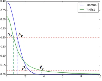
The Student-t distribution is chosen for multiple reasons [vdMH08]. First, t distri-bution is tightly correlated with Gaussian distridistri-bution as it can be decomposed into infinite Gaussian summation. Then the kernel(1 +kyi−yjk2)−1 follows an inverse square law of low-D distance resulting in a larger gap between mapped points of dissimilar data points. Furthermore, the Student-t kernel displays a critical prop-erty as being approximately scale invariant to the change of low-D mapping. And at last,t-SNE is computationally cheaper since it contains no exponential terms. In summary, the natural property of t distribution promotes t-SNE to outperform the original SNE. For outliers,tdistribution’s heavier tails guarantee the robustness

(24)

of low-D probabilities. And principle of weakening the crowding problem can be interpreted as follows. Suppose Gaussian distribution corresponds to the probability in high-D space andtdistribution corresponds to low-D one. We make the best effort to minimize the difference between high-D data manifold and low-D mapping which is to makepij andqij as close as possible. For distant pairwise data pointsiandj in high dimensional space, high-D probabilitypij is smaller than qij taking normalized distance as variable. Thus in order to realizepij =qij, aspij is fixed by high-D data points, a smallerqij is reached corresponding to a further distance that repels low-D mapped points further. Inversely, the close data pointsxi and xj are also attracted closer. Figure 3 illustrates a rough simulation of this pattern between normal andt

distributions.

Figure 3: Influence of tails for close and far apart data points

The cost function of t-SNE is the same as Symmetric SNE

C =KL(PkQ) = X i X j pijlog pij qij

and its gradient is

δC δyi

= 4X j

(pij −qij)(yi−yj)(1 +kyi−yjk2)−1.

van der Maaten discussed further in the following work to alter thet-SNE for high efficiency [vdM14]. A kNN graph was implemented to capture most valuable local data structures in order to reduce the computation expense. He also made clearer

(25)

interpretation of t-SNE by decomposing the gradient of cost function into the at-traction and repulsion terms. Since the gradient with respect toyi was considered as the composition of forces affected onyi, he made the transformation on the gradient that δC δyi =4X j (pij −qij)(yi−yj)(1 +kyi−yjk2)−1 =4X j (pij −qij)qijZ(yi−yj) (3) where Z =P

k6=l(1 +kyk−ylk2)−1 is the normalization term. One step further, it turned out to be

δC δyi = 4(Fattr+Frep) = 4 X i6=j pijqijZ(yi−yj) + X i6=j q_ij2Z(yi−yj) .

The decomposition of gradient inspired van der Maaten to implement tree-based methods such as Barnes-Hut method for optimization acceleration and obtained significant improvements [vdM14]. The related optimization techniques will be in-troduce in Section 4.

t-SNE acquires great popularity since it is proposed for its superiority in data visu-alization splitting crowding clusters to view the unfolded manifold clearly. However,

t-SNE also needs careful tuning of multiple parameters. The optimization process of t-SNE cost function is still tedious and cumbersome with space for promotion. On the other hand, the crowding problem is not perfectly solved byt-SNE yet. This both prompt more innovation on NE algorithm family.

2.5.4 Elastic Embedding

Similar with van der Maaten’s work in t-SNE, Carreira-Perpinán [CP] proposed a generic form of NE cost function decomposing the target into attraction and repulsion terms with a parameterλ indicating the tradeoff. The generic form of cost function is

C =E(Y, λ) =E+(Y) +λE−(Y)

Combining the main notion of NE with the implementation of spectral method, Perpinán also developed a bridge called Elastic Embedding (EE) [CP] between SNE and conventional spectral methods by applying graph Laplacian. For EE, the exact

(26)

cost function is E(Y, λ) = N X i,j pijkyi−yjk2+λ N X i,j exp(−kyi−yjk2)

And the corresponding gradient is

∇E(Y) = 4Y(Lp−λLq) with graph Laplacian terms

Lp =Dp−Wp Lq =Dq−Wq.

HereWp and Wq represent the affinity matrices where elements at ith row and jth column are pij and qij = exp(−kyi−yjk2) respectively. D is the diagonal degree matrix in which the ith element of Dp is D(p)ii =P_jpij. Dq has the same pattern that D(q)ii =

P

jqij.

Yang [YPK14] proved EE being a separable divergence variant of symmetric SNE plus a constant being independent of low-D mappings with Theorem 1 and also gave the best λ value that λ∗ = P

ijpij/

P

ijqij controlling the tradeoff between attraction and repulsion. The spectral nature of EE also allows an out-of-sample plugging-in that is very precious in NLDR.

2.5.5 Weighted Symmetric and t-SNE

At the same time when Theorem 1 is proved, Yang proposes a new variant [YPK14] of symmetric SNE that is closely related to the EE method. This variant starts from modifying the EE method to make the method able to deal with both vectorial data and graph layout. In this variant [YPK14], the edge repulsion strategies borrowed from Noack’s work[Noa07] in graph drawing domain are plugged into the EE [CP] cost function because of its pairwise separable property. Weights M are inserted into the repulsive term in the EE cost function, thus the EE cost function becomes

Cweighted−EE = X ij pijkyi−yjk2+λ X ij Mijexp(−kyi−yjk2)

whereMij =didj and vectorsdi, dj are centrality measures indicating how important the pointsiandj are. Options of centrality measures include closeness, betweenness, degree centrality and eigenvector centrality. Here the degree centrality is selected to represent the point importance. Two disadvantages of weighted EE method are

(27)

that the cost function are sensitive to the scale ofpand parameterλneed a manual tuning. By the flexibility from divergence optimization equivalence, Yang gave a simpler solution that can avoid such disadvantages.

Proposition 2. [YPK14] Weighted EE is a separable divergence minimizing method and its non-separable variant is weighted symmetric SNE (ws-SNE).

Thus a novel variant of SNE can be established with a cost function

Cws−SN E =− X ij pijlnqij + ln X ij Mijqij +const

where const is a constant with none respect to low-D mapping. The selection of

qij is also flexible. Gaussian kernel leads to the weighted symmetric SNE (ws-SNE) while t-distribution kernel turns it to the weighted t SNE (wt-SNE).

ws-SNE and wt-SNE do not treat all the data points equally important, which is very different from original SNE and its early variants. Based on such equal importance assumption, early SNE methods often perform well on vectorial data in neighborhood form for example with pij calculated from kNN graph. However, for graph or network layout of data where there exists highly imbalanced degree centrality, SNE usually displays distorted result. SNE has a tendency to place the more important points of different natural clusters closer which is not proper in reality [YPK14].

Suppose each cluster as a galaxy in the universe space, data points as stars should accumulate tightly in their own galaxy around the galaxy mass core, the center. Meanwhile, there should also exist clear gaps among galaxies. ws-SNE realizes a similar pattern using edge repulsion to divide the clusters more clearly. The gradient of ws-SNE δC δyi =X j pijqθij−cdidjq1+ij θ(yi−yj) where c = P ijpij/( P

ijdidjqij) is the connection scaler where θ = 0 for Gaussian

q, θ = 1 for Student-t q. The first term denotes the attraction composition and the second term for the repulsion with weightsdj and dj. This provides extra repulsion if the data points are more important. The center of one galaxy with greater mass gains greater repulsion from other galaxy centers leading to a farther place. This offers a more significant solution to the crowding problem than the t-SNE using heavy tail shown in [YPK14]. We make a further step combining the heavy tailt(1) a.k.a Cauchy qij with ws-SNE method to explore the performance of this modified setting. The result is shown in Section 6.

(28)

3 Objective and Gradient Approximation

Neighbor embedding methods display better results than the linear and spectral methods but optimization process of NE used to be a great agony since the cost functions and gradients usually are non-convex and computationally expensive. Gen-erally, NE methods attempt to minimize the cost function controlling the mismatch between high-D input data points and low-D mapped points. The mismatch is trans-formed to achieving a balance between the attraction and repulsion forces among the low-D mapped points with optimal tradeoff. In this optimization framework, the exact solution is to compute the the interactions between every pair of mapped data points. Such exact solution is direct but unfeasible since that forN data points, the exact computation has anO(N2) complexity which is easy to cause an overload in memory or a extreme long-run computation. For example, a typical MNIST dataset with 70000 entries may cost 70000×70000×sizeof(double) = 36.5 GB space in memory which is intolerably expensive. Pioneers in NE research applied indirect technique to avoid the O(N2₎_{complexity by only randomly picking a subset of the}

data so that a genral exploration of big dataset can be carried out [vdMH08]. The random subset in summary is not feasible in most cases since it omitted too much information [VCP12]. Thus solution that can accelerate and attack the computa-tion is vital. Fortunately, methods from multiple views have been developed for the improvement and acceleration for the optimization. The first intuition is to avoid computing the exact cost function and gradient.

One common view is applying the methods according to N-body problems in as-trophysics dealing with the gravitational interactions between particles. N-body methods attempts to minimize the potential energy by balancing the particle inter-actions where NE methods has a similar situation trying to minimize the mismatch by getting the optimal tradeoff between attraction and repulsion. All N-body meth-ods with high efficiency are approximate algorithms where tree-based techniques are powerful tools for the acceleration. Two common used methods will be introduced, the Barnes-Hut tree (BH) and Fast Multipole Method (FMM).

(29)

3.1 Barnes-Hut

The cost functions and gradient of NE methods have general form as

C = n X i=1 n X j=1 Aij, δC δyi = n X j=1 Bij(yi−yj)

where Aij and Bij are scalar terms computed between pairwise data points i and j [YPK13]. These terms usually involve coordinates and pairwise distances in output space that vary during the optimization. Considering the summation form in cost function and gradient, one may utilize an approximation solution to reduce the complexity. For data point i, summing up all the interactions between i and all other j points can be divided into summing up multiple interaction subgroups. Interaction produced by each subgroup is approximated by a representative point such as a mass core or a mean.

NE cost functions usually have a summation as

X j f(kyi −yjk2) = X t X j∈Gi t f(kyi−yjk2)≈ X t |Gi_t|f(kyi−yˆtk2)

wherei is the source point, js are the neighbors of i. Gi

t denotes the subgroup that point j belongs to and|Gi

t|indicates how many points are in the subgroup. Suppose gij = f

0

(kyi −yjk2), the gradient can also apply a similar approximation that X j gij(yi−yj) = X t X j∈Gi t gijyi−yj ≈ X t |Gi_t|f0(kyi−yˆtik 2₎₍_y i−yˆti)

If the distance betweeniand subgroupGi

tis far enough, the diversity of interactions betweeniand points in Gi

t will not be significant. Hence all the points inGit will be approximated as one. The interaction complexity is reduced from point-to-point to point-to-group. If we repeat the partition action and implement the approximation to smaller subgroup until only one point left in the group, the interactionf(kyi−yjk2) orgij is directly calculated between pairwise points. Such subgroup partition process follows a route similar to constructing a tree hierarchy.

In practice, multiple techniques can be selected to perform above approximation. A common choice is Barnes-Hut tree based on Quadtree for a 2-D output space. It is quite straight forward to construct a Barnes-Hut tree. Notice that the tree depth is correlated with point density that denser area has deeper tree branches. Each tree

(30)

Figure 4: A Barnes-Hut tree illustration

node contains a subgroup of data points where Gt indicates the points of subgroup or tree node t inside the edge square. For each Gt, if Gt is far away from i, all the interactions of points inside Gt will be composed as |Gt| ×yˆit where |Gt| is the number of points inside node t and yˆi

t is the mean of corresponding points.

One important parameter isθ determining the tradeoff between approximation pre-cision and computational cost. θ achieves such function by deciding how far is far enough for a distance between point i and tree nodet with an inequality

θ·T reeW idth <kyi−yˆitk

where T reeW idth is the edge length of node t’s square. The precision of approxi-mation increases with growing up θ and a typical interval for θ is [1.2,5] [BH86]. Yang successfully applied Barnes-Hut tree in t-SNE acceleration and displayed much better and faster result than random subset method [YPK13]. Since Barnes-Hut has a complexity level of O(NlogN), there still exists space for further improvement.

3.2 Fast Multipole

Barnes-Hut tree generates significant simplification on the optimization complexity from O(N2₎ _to _O₍_N_log_N₎ _{accompanying with some restrictions. First, also the}

most cumbersome one is that the tree size grows exponentially with larger output space dimension, Quadtree for d = 2, Octtree for d = 3, a 2p _{tree for dimension}

(31)

overcome such drawbacks, another N-body method Fast Multipole Method (FMM) based on grid hierarchy is applied by Carreira-Perpinán [VCP14] combining with a grid partition method.

FMM regards the N-body problem as this: with a given set X ⊂ Rd _of _N _target points, a given setY⊂Rd _of_N _{source points, kernel function} _G₍_{x, y}_{), and a weight} set of source points {f(y) :y∈Y}, we want to calculate the potential functionu(t) with respect to every target pointt ∈X as

u(x) = X y∈Y

G(x, y)f(y)

This generic form appears in many research domains, for example in astrophysics, X=Yindicate the sets ofN stars,G(x, y) = 1/|x−y|is the gravitational potential. Direct computation ofu(x)requiresO(N2)and it’s rather expensive whenN is large. FMM abandons the direct method of brute forces. It decomposes the interactions among target and source points with a 3-stage process as (1)accumulation, (2)shift, (3)expansion for an approximation. Suppose that the dataset distributes in a square [0,1] × [0,1] with normalization and A, B are subsquares of same size without overlapping. The three stage process is shown in Figure 5.

Figure 5: FMM 3 Stages

The first stage accumulation composes the source points in B to the center cB. Then shift the composed effect to the center cA of target point in A establishing a

(32)

square-square interaction. Finally, execute the expansion on cA for approximation. Usually, the dataset is normalized in a square and a grid frame is established to ensure the number of points in every square smaller than a threshold.

Carreira-Figure 6: Grid Establishment

Perpinán applied FMM to approximate the cost function and gradient in his work [VCP14]. The Fast Gaussian Transform(FGT) is taken as a generic kernel form as

Q(yi) = N

X

j=1

qjexp(−k(yi−yj)/σk2)

Recall the cost function of Elastic Embedding that

C(Y) = N X i,j=1 ωijkyi−yjk2+λ N X i,j=1 exp(−kyi−yjk2)

The kernels of cost function and its gradient can both be expressed with modification of the FGT indicating the interaction kernel as G(x, y)introduced above.

Carreira-Perpinán first normalized the dataset to a unit box [0,1] and partitioned the box with grids. Instead of expanding the interaction form the source points center to the target points center, Carreira-Perpinán did the series expansion locally around EVERY point with a Hermite expansion

exp(−k(t−s)/σk2_{) =} ∞ X k=0 1 k!hk( s−sc σ )( t−sc σ ) k

where t is the target point and s is the source point. hk(x) = e(−x 2₎

Hk(x) are the Hermite functions with Hermite polynomials Hk(x). The parameter k controls the tradeoff between precision and computation cost, for a greater k the precision increases and it requires more computation.

(33)

Compared with Barnes-Hut tree, though FMM is claimed being able to realize an

O(N) complexity, it still remains some suspicions. Suppose the uniform box[0,1]is partitioned into m subsquares, by Carreira-Perpinán’s method, each subsquare will execute the 3-stage expansion on every point. The entire computation then gets a complexity of O(mN). Though the complexity O(NlogN) has not been strictly proved for Barnes-Hut tree, O(mN) of FMM does not always outperform Barnes-Hut tree. For example, theM N IST dataset with 70000 entries has a approximate complexity ofNlogN ≈12×70000. While for FMM, the number of subsquares will easily surpass 12if the grids are tiny enough. Moreover, FMM for NE methods are not feasible for heavy-tailed qij since the expansion is only applicable for light-tail distributions and relies on their fast decaying property [YPK13]. So, for simplicity and scalability, we apply the Barnes-Hut tree as the approximation techniques in our following works.

4 Optimization

With the approximation of cost function and gradient, the complexity of optimiza-tion process decreases to be acceptable. Early developed NE methods applied mul-tiple variants of straight gradient descent methods with numbers of parameters to tune such as the learning step size of gradient descent method and the momentum of annealing simulation. However, it is quite tricky to get the optimal values for such parameters and a long-run optimization may be repeated again and again. Furthermore, the parameters usually highly rely on the certain dataset and are not portable meaning that when the dataset changes, the parameters need to be tuned again. Thus optimization techniques for NE with few or no parameters are developed to avoid the tuning tricks. Three optimization methods that will be dis-cussed in following parts are fixed point [YKXO09], partial Hessian [VCP12] and majorization-minimization [YPK15]. All these methods can provide results that are at least as good as gradient descent methods but much simpler to realize.

4.1 Fixed Point

Optimization based on fixed point borrows the concept of fixed point whose defini-tion is that [GD13]: for a given funcdefini-tion ϕ, if ϕ(x∗) =x∗, then x∗ is a fixed point of ϕ. In the other words, the fixed point of ϕ is the intersection point of function

(34)

curve ϕ(x) and straight line y=x.

The optimization of cost function by fixed point method is fundamentally a root finding problem that is looking for the zero point of corresponding gradient repre-senting the location of the optima. This can be done following the general path of fixed point iteration which transforms a root-finding problem to a fixed-point finding problem.

The basic setting of fixed point iteration is this: For target function f(x) = 0, construct an equivalent function x =ϕ(x) where the root of f(x) = 0 is equivalent to the fixed point ofϕ(x). And the iteration follows the procedure as for an arbitrary initial value x0, compute

xk+1 =ϕ(xk) k = 0,1,2,· · ·

hence an iterative seriesx1, x2,· · · , xn,· · · is obtained approaching the fixed point. Figure 7: Brief illustration of fixed point iteration

Figure 7 shows an illustration of fixed point iteration. However, in practical work, the convergence of such iteration is not always assured. It requires certain conditions to perform the convergence following a theorem as

Theorem 2. [GD13] Assume ϕ(x)∈C[a, b] and satisfies (1) for ∀x∈[a, b], there is ϕ(x)∈[a, b]

(2) there exists a constant L that for ∀x, y, it satisfies

|ϕ(x)−ϕ(y)| ≤L|y−x|

Then for arbitrary initial value x0, the fixed point xk+1 = ϕ(xk) converges and has

the bounds as |xk−x∗| ≤ L 1−L|xk−xk−1| ≤ Lk 1−L|x1−x0|.

(35)

It has also been proved that the above convergence is a global property and in general a smallerLbrings faster convergence. Figure 8 shows a divergent process of fixed point iteration that does not satisfy the convergence conditions.

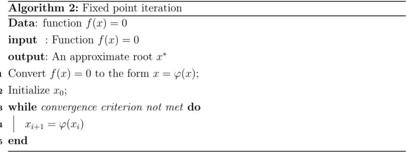
The corresponding pseudo code for fixed point iteration is Algorithm 2: Fixed point iteration

Data: functionf(x) = 0 input : Function f(x) = 0 output: An approximate root x∗

1 Convert f(x) = 0 to the form x=ϕ(x); 2 Initializex0;

3 while convergence criterion not met do 4 xi+1 =ϕ(xi)

5 end

Figure 8: Example of diverge fixed point iteration

Implementation in NE

The details of implementing fixed point method to optimize the cost function of NE are interpreted in [YKXO09]. In this article, a general gradient function of different heavy-tailed low-D probability distribution is proposed, which is not only restricted to the t distribution with 1 degree of freedom. Recall the optimization task for symmetric NE methods, the target or the cost function has the form

C(Y) = DKL(PkQ) = X i6=j pijlog pij Qij

(36)

where Qij = qij/

P

k6=lqkl are the normalized low-D similarities. The cost function can be transformed to an equivalent form as

maximize q,Y L(q, Y) = X ij pijlog qij P k6=lqkl subject toqij =H(kyi−yjk2)

whereH(τ)is the embedding similarity function which can be any function as long as it is monotonically decreasing with respect to positive τ. By adding Lagrangian multiplier to the equivalent cost function, we can get the gradient with respect to

yi as ∂C(Y) ∂yi = 4X j (pij −Qij)S(kyi−yjk2)(yi−yj) where h(τ) = dH(τ)/dτ and S(τ) = −dlogH(τ) dτ

is the negative score function of H and we denote Sij =S(kyi−yjk2).

FunctionS can be considered as the tail-heaviness function and H is the similarity function. The heavy-tailed distribution family thus can be written as

H(τ) = (ατ +c)−1/α

where a larger α indicates heavier tails. Gaussian similarity takes α = −1, c = 0 and Student-t(1) has α= 1, c = 1.

With the above generic form of heavy-tailed SNE family, the iterative update solu-tion is given by setting the partial derivative of cost funcsolu-tion ∂C/∂yi = 0 as

Y_ki(t+1) = Y (t) ki P jBij + P j(Aij −Bij)Y (t) kj P jAij whereAij =pijS(ky (t) i −y (t) j k2)and Bij =QijS(ky (t) i −y (t)

j k2). The iterative update for Y_kj(t+1) can be derived by setting ∂C/∂yj = 0.

Still the convergence of fixed point ietration is not guaranteed and Yang did a deep discussion in [YKXO09] in which two theoretical justifications of algorithm approximation were provided.

(37)

4.2 Spectral Direction

Another popular technique to cope with such non-linear optimization problem is Newton method. Different from the gradient descent methods with first order con-vergence applied in early NE works, Newton method performs second order conver-gence showing a much higher speed to converge. A lot of variants originated from Newton method have achieved great successes in many research domains. The basic idea of standard Newton method is that: at the current minimum value, we carry out a second order Taylor expansion according to target function f(x) in order to find out next closer location of global optima. Now suppose our current location is

xk, then we denote ϕ(x)≈f(xk) +∇f(xk)·(x−xk) + 1 2(x−xk) T _{· ∇}2_f₍_x k)·(x−xk)

as the second order Taylor expansion off(x)aroundxk. Here∇f(xk)is the gradient and ∇2_f₍_x

k)is the Hessian matrix. For notation simplicity, ∇f(xk) is expressed as

gk and ∇2f(xk) asHk.

Due to the essential condition of being an optima, ϕ(x) should satisfy ∇ϕ(x) = 0 which means by adding gradient operator on both sides of above expansion, the following is obtained

gk+Hk(x−xk) = 0. Furthermore, ifHk is non-singular, we can get a solution

x=xk−H_k−1gk.

Hence the iterative procedure for optimization is constructed with a given initial point x0 as

xk+1 =xk−ηk·Hk·gk=xk+ηk·dk, k = 0,1· · ·

where dk =−Hk·gk is called search direction. ηk is the step size determined by a line search to avoid the procedure falling into poor local optima or diverging. The step size has the property that

ηk= arg min

η∈Rf(xk+η·dk).

In most cases, Hessian mstrix Hk or its inverse Hk−1 is very hard to be computed directly. A compromise is to use the approximation of Hessian and the correspond-ing Quasi-Newton method turns to be attractive. Prevalent Quasi-Newton methods

(38)

include DFP [Dav91], BFGS [SK70] and L-BFGS [LN89]. DFP algorithm approx-imates H_k−1 while BFGS and L-BFGS directly approximate Hk iteratively. BFGS keeps the history of first order gradient during the iterations to obtain more accurate result. L-BFGS is the realization of BFGS on huge dataset where how long would the history be kept can be manually chosen to balance the memory consumption and computation precision.

The notion of Quasi-Newton is also feasible in NE optimization because Hessian is able to be well approximated by a graph Laplacian [BN01] with probabilistic prox-imities encoded within. Carreira-Perpinán proposed specific way to carry out Quasi-Newton for NE problems [VCP12]. Recall that Carreira-Perpinán decomposed the cost function as

C =E(Y, λ) =E+(Y) +λE−(Y)

where E+₍_Y₎ _{is the attractive part and} _E−₍_Y₎ _{denotes the repulsion.}

In most cases a complete Hessian of cost function is not necessary and the spectral direction (SD) is purely yielded from the Hessian of attractive part ∇2_E+₍_Y_{) =}

4L+⊗Id which is positive semi definite and consisting of d×d identical diagonal blocks of N ×N with d being the dimension of low-D space. Graph Laplacian L+

plays an important role in construction the search direction.

Even with the partial Hessian, implementing Quasi-Newton is still often cumber-some. Perpinán in his work applied some more tricks for improvement. First, the Hessian is sparsified to k nearest neighbors. Then small positive is added to the diagonal of partial Hessian to guarantee the positive definiteness. At last, instead of calculating search direction dk = −B_k−1·gk where Bk is the partial Hessian, he tried to solve a linear systemBk·dk=−gk. For better performance, a Cholesky de-composition is executed onBk turning the system toRTk·Rk·dk =−gk. After twice backsolving, the search direction or the spectral direction is acquired. Then follow-ing other Quasi-Newton steps, the optimization is carried out. For more details, please see [VCP12] and its supplement.

(39)

4.3 Majorization-Minimization

Besides Newton method, Majorization-Minimization (MM) [OR00] is also an op-timization technique that can apply the second order convergence. The prevalent Expectation-Minimization (EM) algorithm [DLR77] is just a special case of MM al-gorithm. The main idea of MM algorithm is simple that if the target function J(x) is hard to optimize, we will seek a replacement function G(x) which is simpler to optimize. As long as G(x) satisfies the following three conditions, the minimum of target function J(x)thus can be infinitely approximated by the minimum of G(x). The conditions G(x)should satisfy are

• G(x) is easy to optimize.

• At stepk, Gk(x)≥J(xk)for all x.

• G(xk) = J(xk)

For a minimization procedure, G(x) majorizes the target functionJ(x)and “slides” on J(x) during the iteration. The iteration for optimization can be described as below

1. Set k = 0, initialize x0.

2. Choose Gk such that Gk(x)≥J(xk)for all xand Gk(xk) =J(xk). 3. Set xk+1 as the minimizer ofGk(x).

4. Set k =k+ 1 and go to Step 2.

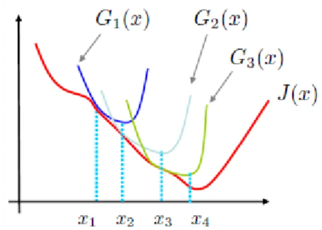
Figure 9 illustrates the optimization iteration. From the above description we can see the key point to apply MM method is whether we can construct a tight majoriza-tion or bound of the target funcmajoriza-tion. Many matured solumajoriza-tions have been proposed including quadratic bound, Lipschitz upper bound, Jensen’s inequality etc.

The implementation of MM method in NE also relies on the decomposition of cost function [YPK15]. Now assume the cost function can be divided into two parts

(40)

Figure 9: Majorization-minimization iterative process

HereY,Y˜, andYnew _{denote the current estimate, the variable and the new estimate} respectively. The proximities Qand Q˜ are computed from the current estimate and the variable respectively.

The A(P,Q˜) term can be upper bounded by a summation of quadratic pairwise terms thatA(P,Q˜)≤P

ijWijky˜i−y˜jk2+constant where the multipliersWij do not depend onY˜. PartB(P,Q˜)has an Lipschitz surrogate upper bound ashΨ,Y˜−Yi+

ρ

2kY˜ −Yk

2_{+constant where} _{Ψ =} ∂B

∂Y˜|Y˜=Y and ρ is the Lipschitz constant.

With the above upper bounds based on quadratification and Lipschitzation, the majorization functionG( ˜Y , Y) is thus constructed where

G( ˜Y , Y) = X ij Wijky˜i−y˜jk2+hΨ,Y˜ −Yi+ ρ 2k ˜ Y −Yk2₊_const

Setting the gradient ofG( ˜Y , Y)with respect toY˜ to zero and solving forY, we can get the iterative update rule

Ynew = (2LW+WT +ρI)−1(−Ψ +ρY) where L_W₊_WT denotes the graph Laplacian of matrix W +WT.

Taking the implementation of MM in t-SNE as an example. In t-SNE, A(P,Q˜) =

P ijPijln(1 +ky˜i−y˜jk2) and B(P,Q˜) = ln P ij(1 +|y˜i−y˜jk2)−1 where qij = (1 + kyi−yjk2)−1 and Q˜ij = (1+|yi˜−yj˜ k2₎−1 P

kl(1+|yk˜ −yl˜k2)−1. The corresponding update rule is

Ynew= (LP◦q+ ρ 4I) −1_(L Q◦q+ ρ 4Y)

(41)

where Lagain denotes the graph Laplacian and ◦ is the elementwise product oper-ator.

In practice, MM is realized by two loops: an outer loop for the update ofY and an inner loop to search for the Lipschitz constant ρ. Different from spectral direction (SD) method where a smallis heuristically added to ensure the positive definiteness of Hessian, MM applies an adaptive process to determine ρ which brings greater robustness and accuracy [YPK15].

5 Implementation

We manage to realize the Weighted t-SNE with majorization-minimization frame-work (wtsnemm) method in statistic software R. Some frame-works have been done to perform NE method in R such as the tsne package developed by van der Maaten. However most of these early works focus on a specific NE variant and are not well improved. Thus we determine to realize the Weighted t-SNE which can provide better visualization and apply majorization-minimization to achieve faster, more accurate and robust output. Also, a package is built to wrap all the functions and source codes in order to strengthen the portability. The details of NE method implementation and package build will be shown in the following parts.

R, a.k.a GNU S, is a free and open source platform and language for statistical computing and visualization. Hence it has active communities and users developing extensions to accomplish a variety of statistical tasks. Besides directly sharing the work by other users from official Comprehensive R Archive Network (CRAN), R allows users to write their own extensions to cope with specific problems. Such flexibility comes from the fact that R is able to communicate with multiple popular programming languages such as Python, Java and Scala. Fortran and C/C++ can be conveniently involved in R codes to achieve significant scalability and efficiency improvements. In this article, our work is done by applying both R language and C++ to acquire both high efficiency and easy manipulation. The R version used in this work is 3.3.3.