Accepted Manuscript
Possibilistic and fuzzy clustering methods for robust analysis of non-precise data
Maria Brigida Ferraro, Paolo Giordani
PII: S0888-613X(17)30293-1
DOI: http://dx.doi.org/10.1016/j.ijar.2017.05.002
Reference: IJA 8056
To appear in: International Journal of Approximate Reasoning Received date: 28 June 2016
Revised date: 2 May 2017 Accepted date: 2 May 2017
Please cite this article in press as: M.B. Ferraro, P. Giordani, Possibilistic and fuzzy clustering methods for robust analysis of non-precise data,Int. J. Approx. Reason.(2017), http://dx.doi.org/10.1016/j.ijar.2017.05.002
This is a PDF file of an unedited manuscript that has been accepted for publication. As a service to our customers we are providing this early version of the manuscript. The manuscript will undergo copyediting, typesetting, and review of the resulting proof before it is published in its final form. Please note that during the production process errors may be discovered which could affect the content, and all legal disclaimers that apply to the journal pertain.
Highlights
• A robust clustering method for imprecise data is proposed
• The clustering process is based on fuzzy and possibilistic approaches
• Imprecision is managed in terms on fuzzy sets
Possibilistic and fuzzy clustering methods for robust
analysis of non-precise data
Maria Brigida Ferraro, Paolo Giordani
Dipartimento di Scienze Statistiche, Sapienza Universit`a di Roma, P.le Aldo Moro, 5 - 00185, Rome, Italy
Abstract
This work focuses on robust clustering of data affected by imprecision. The imprecision is managed in terms of fuzzy sets. The clustering process is based on the fuzzy and possibilistic approaches. In both approaches the ob-servations are assigned to the clusters by means of membership degrees. In fuzzy clustering the membership degrees express the degrees of sharing of the observations to the clusters. In contrast, in possibilistic clustering the mem-bership degrees are degrees of typicality. These two sources of information are complementary because the former helps to discover the best fuzzy par-tition of the observations while the latter reflects how well the observations are described by the centroids and, therefore, is helpful to identify outliers. First, a fully possibilistic k-means clustering procedure is suggested. Then, in order to exploit the benefits of both the approaches, a joint possibilistic and fuzzy clustering method for fuzzy data is proposed. A selection proce-dure for choosing the parameters of the new clustering method is introduced. The effectiveness of the proposal is investigated by means of simulated and real-life data.
Keywords: Imprecise information, Robustness, Fuzzy clustering, Possibilistic clustering, Cluster validity.
1. Introduction
In most practical applications the results of the statistical analysis may be poor due to some outliers or other departures from the ideal conditions on which the statistical methods are based. In the cluster analysis framework, the presence of contaminated data is usually deleterious: a limited number
of outliers may lead to a completely wrong and inaccurate partition of the observations. In this work, following the fuzzy approach and the closely related possibilistic one, some robust clustering procedures will be proposed. In doing so, we assume to deal with a special kind of data, i.e., non-precise data. A fruitful way to handle imprecision is by means of fuzzy sets [1, 2, 3]. In this connection, it is important to distinguish between the epistemic and ontic nature of the fuzzy data. In the epistemic approach fuzzy data are seen as imprecise measurements of precise data. Thus, the available information on a precise quantity is ill-known and the lack of precision is managed through fuzzy sets. In the ontic approach fuzzy data are seen as whole entities, hence the quantity under investigation is assumed to be intrinsically imprecise. In practice, the distinction between the epistemic and ontic fuzzy sets has a relevant impact on the statistical tools to apply. See, for more details, [4, 5]. In this work we assume to deal with ontic fuzzy sets.
A lot of standard clustering procedures have been generalized to the fuzzy data case. The use of belief functions in the clustering process is considered in [6]. Clustering fuzzy data by means of mixtures of distributions is suggested in [7, 8]. The large majority of the proposals are based on the fuzzy k-means algorithm and consist mainly in introducing suitable dissimilarity measures for fuzzy data [9, 10, 11, 12, 13, 14, 15, 16, 17, 18, 19]. Robust clustering methods for fuzzy data can be found in [20, 21, 22, 23, 24, 25]. These are robust versions of the fuzzy k-means algorithm for such a kind of data and can be distinguished with respect to the approach adopted for handling the outliers. In the precise data case, these can be roughly summarized as follows (we refer to the review in [26] for a deeper insight). An approach consists in the use of medoids (see, e.g., [27]). This is a a timid kind of robustification because it does not explicitly manage contaminated data reducing their in-fluence in the clustering process [28]. An alternative approach is represented bytrimming(see, e.g., [29]). The key idea is to simultaneously discard a pro-portion of observations and to apply the clustering procedure on the clean data. Thus, in the trimming approach the observations are considered either outliers or not. A softer approach allowing the existence of “outliers to a certain extent” consists in adding a noise cluster to the k “good” clusters [30]. The role of the noise cluster is that the outliers will be assigned to it with high membership degrees and, therefore, will have small membership degrees to the “good” clusters. A distinct approach is represented by the use of metrics able to mitigate the influence of outliers (see, e.g., [31, 32]). A different strategy is offered by the possibilistic approach [33]. Its peculiarity
is that the membership degree is only based on the distance between the observation and the involved centroid. Hence, the outliers, far from the bulk of the data, will have low membership degrees to all the clusters (see, for a deeper insight, [33]).
In this work, following the possibilistic approach, two new robust fuzzy clustering methods for fuzzy data will be proposed. The first method is fully possibilistic. However, as we will see, it may suffer from the risk of obtain-ing coincident clusters, i.e., clusters characterized by the same centroids. To overcome this problem, a second robust method is introduced preventing the occurrence of coincident clusters. The outline of the paper is as follows. In the next section we recall the theory of fuzzy sets describing the general fam-ily of LR fuzzy data and a dissimilarity measure for LR fuzzy data. Then, we discuss the concept of fuzzy data outliers. In Section 3 we recall the fuzzy k -means algorithm for LR fuzzy data [22] and propose a possibilistic clustering method for LR fuzzy data. Since it is not guaranteed that coincident clusters do not occur, the so-called possibilistic fuzzy clustering method for LR fuzzy data (PFkM-F) is suggested in Section 4. A selection procedure for choosing the parameters to be used in PFkM-F is discussed in Section 5. The effec-tiveness of the proposal is illustrated in Section 6 by means of a simulation study and some applications to real data. Finally, some concluding remarks are made in Section 7.
2. Fuzzy data
A fuzzy setX is identified by a membership function μX(z), i.e. a map-ping μX(z) : R → [0,1] (see [1]). Let Kc(R) be the class of non-empty compact convex subsets ofR, the class of fuzzy numbers isFc(R) ={μX(z) :
R →[0,1] : Xα ∈Kc(R)}, where Xα is the α-level set of X. For 0< α ≤1, it can be defined as the non-empty compact convex subset of R such that
Xα = {z :μX(z)≥ α}. For α= 0, X0 =cl({z :μX(z) >0}) (cl() indicates the closure of a set).
The most common class of fuzzy numbers is the LR one. In this case, the generic fuzzy datum X can be defined by four parameters, namely the left center (c1), the right center (c2), the left spread (l >0) and the right spread (r >0), and the following membership function:
μX(z) = ⎧ ⎨ ⎩ Lc1−z l z ≤c1, 1 c1 ≤z ≤c2, Rz−c2 r z ≥c2, (1)
Trapezoidal l r c1 c2 0 1 Interval l = r = 0 c1 c2 0 1 LR fuzzy set l r c1 c2 0 1 Crisp l = r = 0 c1=c2 0 1 Triangular l r c1=c2 0 1
Figure 1: An LR fuzzy number and its specific cases. From the top in clockwise direction, a trapezoidal fuzzy number, a crisp number, a triangular fuzzy number and an interval are reported.
where the function L:R→[0,1] (andR) is a convex upper semi-continuous function so that L(0) = 1 and L(z) = 0, for all z ∈ R\[0,1]. The centers provide information about the location of the fuzzy datum, whilst the spreads inform us about the associated imprecision (the size). If L(z) = 1−z and
R(z) = 1−z for 0≤z ≤1, then X is a trapezoidal fuzzy number when
c1 =c2 and a triangular fuzzy number when c1 = c2 = c. If l = r = s = 0, then X is a symmetric LR fuzzy number. If c1 = c2 and l = r = 0 we get an interval. Finally, a crisp number (non-fuzzy datum) is obtained when
c1 = c2 = c and l = r = 0. All the above specific cases are represented in Figure 1.
When p LR fuzzy variables are collected on a set of n observations, we have the fuzzy data matrix
X=
Xij ≡(c1ij, c2ij, lij, rij)LR, i= 1, ..., n, j = 1, ..., p , (2) where Xij ≡ (c1ij, c2ij, lij, rij)LR represents the j-th LR fuzzy variable col-lected on thei-th observation with left centerc1ij, right centerc2ij, left spread
lij and right spreadrij. We can define the matrices of the left centers (C1), of the right centers (C2), of the left spreads (L) and of the right spreads (R) of order (n×p) with generic elementsc1ij, c2ij,lij and rij, respectively. Hence,
˜
xi ≡(c1i,c2i,li,ri)LR is the fuzzy vector of length pfor observation i, where
˜
xi, c1i, c2i, li and ri are thei-th rows of X, C1, C2, L and R, respectively.
2.1. Dissimilarity measures for fuzzy data
In order to develop clustering methods for LR fuzzy data we need a suitable dissimilarity measure. We adopt the one introduced in [22]. It is defined as a weighted sum of the (squared) Euclidean distances between centers and spreads. In detail, given two LR fuzzy observations, xi and xi we have
d2w(xi,xi) =w2[d2(c1i,c1i) +d2(c2i,c2i)] + (1−w)2[d2(li,li) +d2(ri,ri)], (3) where d(·,·) is the standard Euclidean distance (for non-fuzzy data), w and 1−ware weights for the center component and the spread component, respec-tively. By means ofd2w(xi,xi) we compute the dissimilarity between two LR fuzzy observations as the weighted sum of the squared Euclidean distances for the (left and right) centers and the (left and right) spreads. The weights
w and 1−w must be non-negative. Moreover, taking into account that the membership function takes the maximum value in the centers, they must be such that the distances for the centers play a more relevant role than those for the spreads, hence, w ≥ 1−w ≥ 0. It follows that w must belong to [0.5,1] (and 1−w to [0,0.5]). As we shall see, w will be estimated within the clustering problem. It must be underlined that (3) is utilized for evalu-ating the existing differences among observations belonging to a given data set and, therefore, the estimated weight is optimal only for the involved data set.
Remark 1. The squared dissimilarity in (3) is valid for the general class
of LR fuzzy numbers. Some particular cases are worth mentioning. For in-stance, in the case of triangular fuzzy data, (3) can still be applied. When we have symmetric triangular fuzzy data (3) reduces to the squared dissimilarity proposed in [19]. Finally, in case of non-fuzzy data, (3) coincides with the squared Euclidean distance.
2.2. Fuzzy data and outliers
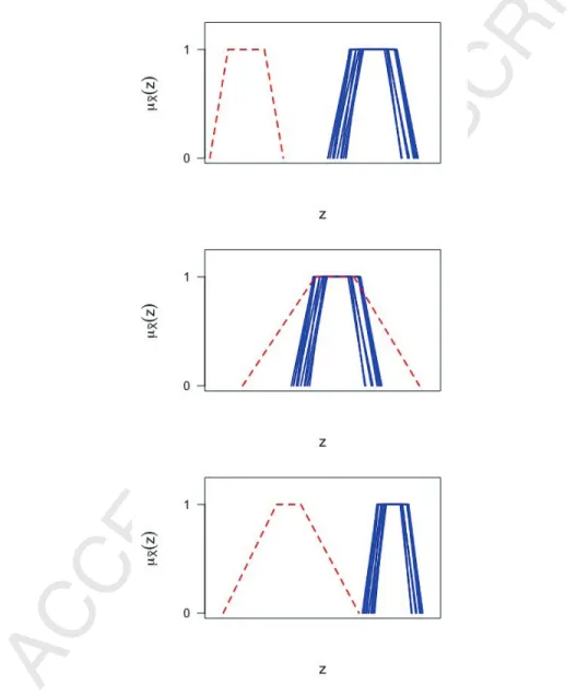
There exist different kinds of contamination. Fuzzy data can be consid-ered outliers with respect to their centers (see top of Figure 2). In this case the contamination is due to the location. Another kind of contamination is
Figure 2: From top to bottom: outlier w.r.t. center, outlier w.r.t. spread, outlier w.r.t. center and spread (red dashed line).
spreads. Finally, there are outliers with respect to both centers and spreads (see bottom of Figure 2), that are outliers due to both the location and the size. When clustering fuzzy data we should apply methods able to mitigate the distortion produced by all these kinds of contamination.
3. Fuzzy and possibilistic k-means algorithms for fuzzy data
In order to clustern observations described by p LR fuzzy variables, the fuzzy k-means clustering method for LR fuzzy data (FkM-F) proposed by Coppi et al. [22] can be applied. The FkM-F optimization problem can be written as min U,H,w JF kM−F = n i=1 k g=1 umigd2w xi,hg , (4) s.t. uig ≥0, i= 1, . . . , n, g = 1, . . . , k, (5) k g=1 uig = 1, i= 1, . . . , n, (6) w∈[0.5,1], (7)
where uig is the membership degree of observation i to cluster g, stored in the matrix U of order (n×k), and
H= Hgj ≡ hC1 gj, h C2 gj, h L gj, h R gj LR, g = 1, ..., k, j = 1, ..., p . (8) In (8) Hgj ≡ hC1 gj, h C2 gj, hLgj, hRgj
LR represents the j-th LR fuzzy variable for the g-th centroid with left center hC1
gj, right center h C2
gj, left spread hLgj and right spread hR
gj. We can define the centroid matrices of the left centers (HC1), of the right centers (HC2), of the left spreads (HL) and of the right spreads (HR) of order (k×p) with generic elements hC1
gj, h C2
gj, hLgj and hRgj, respectively. Therefore, ˜hg ≡ (hCg1,hgC2,hLg,hRg)LR is the fuzzy vector of length p for centroid g, where h˜g, hCg1, hCg2, hLg and hRg are the g-th rows of
H, HC1, HC2, HL and HR, respectively. Thus, the centroids are assumed to have a complex structure inherited from the observed data. In other words, the imprecision of the observed data is propagated to the centroids that are of fuzzy nature. The squared dissimilarity d2w
xi,hg
recalled in (3) is used for comparing observation i with centroid g. Finally, m > 1 is the fuzziness
parameter. The membership degrees of the observations to the clusters are such that they are inversely related to therelative dissimilarities between the observations and the centroids. For this reason, the membership degrees can be interpreted as degrees of sharing (of the observations to the clusters).
In case of outliers, the fuzzy approach fails due to the unit-sum constraints of the membership degrees. By relaxing these constraints we move from the fuzzy to the possibilistic approach [33]. The so-called possibilistic k-means clustering method for LR fuzzy data (PkM-F) can be formalized as
min T,H,w JP kM−F = n i=1 k g=1 tηigd2w xi,hg + k g=1 γg n i=1 (1−tig)η, (9) s.t. tig ∈[0,1], i= 1, . . . , n, g = 1, . . . , k, (10) w∈[0.5,1], (11)
wheretig is the membership degree of observationito clusterg, stored in the matrixTof order (n×k). As for the standard possibilistick-means clustering method for non-fuzzy data [33], the membership degrees are possibility values and are usually referred to as the degrees of typicality (of the observations to the clusters), although, as an anonymous reviewer noted, tig is not a possibility value in a strict sense because, for the generici-th observation,tig’s should be normalized so that max
g tig = 1. γg is a cluster-specific parameter tuning the importance of the clusters and η (> 1) is the fuzzifier. The parameter γg can be defined as
γg =γ n i=1 um igd2w xi,hg n i=1 um ig , g = 1, . . . , k, (12)
where, usually, γ = 1 and hg’s and uig’s are obtained from FkM-F. (12) can be motivated by noting that the γg’s give the relative weight of the second term of the loss compared to the first one. The second term avoids the trivial solution with T = 0. When the γg’s have approximately the same order of thed2w
xi,hg
’s, then the two terms of the loss are weighted roughly equally. The values of the γg’s differ among clusters and depend on their overall sizes and shapes. The choice of the γg’s determines the zones of influence of the clusters. In particular, γg gives the dissimilarity at which the degree of
typicality of an observation to clusterg becomes 0.5. Whenγg is low or high, we expect degrees of typicality tig’s low or high, respectively.
The solution of PkM-F can be derived by using the iterative algorithm proposed in the next section. In PkM-F the degrees of typicality are in-versely related to the absolute dissimilarities between the observations and the centroids. In fact, a common property of clustering methods based on the possibilistic approach is that the membership degrees are computed by considering only the dissimilarity between the observation and the involved centroid, regardless of the centroids of the remaining clusters. Intuitively, this clarifies how the possibilistic approach well manages contaminated data. Outliers are far from the bulk of the data and, thus, far from all the cen-troids. Therefore, they usually have degrees of typicality close to 0 to all the clusters (see, for an deeper discussion, [33]).
The PkM-F problem is a novel clustering method and represents an ex-tension to the fuzzy data case of the algorithm introduced in [33]. Note, however, that PkM-F is not the first possibilistic clustering method for LR fuzzy data proposed in the literature. In fact, taking inspiration from [39], Coppi et al. [22] propose a different possibilistic clustering method for fuzzy data (hereinafter, C-PkM-F). The PkM-F and C-PkM-F methods can be formulated in the same way except for the second term of the cost function. Such a second term (not reported here for C-PkM-F) avoids solutions with
T=0.
Although the possibilistic approach to clustering works well, it suffers from a well-known limitation, i.e., the risk of obtaining a trivial solution with coincident clusters [34]. Since the sum of the degrees of typicality for every observation to all the clusters is no longer required to be equal to one, it may occur that the centroids of the clusters are the same. This can be explained by noting that the loss functions of the possibilistic procedures can usually be decomposed into the sum of k terms (one for every cluster) that can be minimized independently of each other. It is easy to show that such a comment holds for PkM-F and C-PkM-F. A heuristic remedy to the coinci-dent cluster problem is the use of a rational starting point. For instance, the iterative algorithm of PkM-F can be run starting from the FkM-F solution. This strategy has also been adopted for C-PkM-F. Although very common, this remedy does not always exclude the occurrence of trivial solutions with coincident clusters.
It should be clear that in practical applications PkM-F will be rarely used. Nonetheless, it is useful to derive the here-proposed clustering method.
More specifically, in order to solve the coincident clustering problem, at least two strategies can be followed. The first one consists in adding a repulsion term among centroids in the loss function. Such a repulsion term forces the centroids to be far from each other. In [23] a possibilistic clustering method with repulsion constraints for symmetric triangular fuzzy data is developed. Its extension to the general family of LR fuzzy data is not straightforward. A different strategy for preventing coincident clusters is the hybridization of the fuzzy and possibilistic approaches, namely of FkM-F and PkM-F, exploiting their potentialities and overcoming their drawbacks. This is pursued in this work.
4. Possibilistic fuzzy k-means algorithm for fuzzy data
The possibilistic fuzzy k-means clustering method for LR fuzzy data (PFkM-F) can be formalized as min U,T,H,w JP F kM−F = n i=1 k g=1 aumig +btηigd2w xi,hg + k g=1 γg n i=1 (1−tig(13))η, s.t. uig ≥0, i= 1, . . . , n, g = 1, . . . , k, (14) k g=1 uig = 1, i= 1, . . . , n, (15) tig ∈[0,1], i= 1, . . . , n, g = 1, . . . , k, (16) w∈[0.5,1], (17)
where m >1 denotes the parameter of fuzziness andη and γg have the same meanings discussed in PkM-F. The idea underlying PFkM-F is to exploit the potentialities of FkM-F and PkM-F. This goal is achieved by minimizing a cost function which is a linear combination of those of FkM-F and PkM-F, respectively, with weights given by a and b, respectively. The non-negative quantities a and b tune the relative importance of the degrees of sharing (in U) and of the degrees of typicality (in T) in the objective function. These two sources of information are not exclusive because they jointly allow for a thorough analysis of the cluster structure. The matrix T helps to detect outliers. Generally speaking, an observation can be considered an outlier when all its degrees of typicality are low. In addition, the fuzzy partition of the observations can be assessed by looking at U. The non-negative parameters a and b tune the importance of the degrees of sharing
and typicality in the clustering process. The highera(b) is, the more relevant is the emphasis of the fuzzy (possibilistic) approach. In fact, if a is high, then the centroids (in H) mainly depend on the degrees in U. Similarly, if
b is high, the degrees inT remarkably influence the centroids. Therefore, in order to reduce the effect of outliers, a larger value ofbcan be set. Coincident clusters could occur for large values ofb, but the problem can easily be solved by increasing a. In other words, the simultaneous use of FkM-F and PkM-F allows to eliminate the drawbacks of the two methods. On the one hand, the FkM-F part of the cost function avoids (for sufficiently large values of
a) that the centroids are coincident and therefore the degrees of typicality have a practical meaning. On the other hand, the PkM-F part mitigates the influence of the outliers in the obtained partition. In case of particularly large values of a and b, it might be convenient to select a high value for
γ in (12) to avoid that the second term of (13) plays a negligible role in the clustering process. For a deeper insight into the properties of clustering methods jointly based on the fuzzy and possibilistic approaches the interested reader may refer to [35, 36].
Remark 2. A lot of existing clustering methods can be obtained as special
cases of PFkM-F. If b = 0 and γg = 0, g = 1, . . . , k, then we obtain FkM-F [22], while for a = 0 the problem coincides with PkM-F. When PFkM-F is run using non-fuzzy data (i.e., X ≡ X with C1 =C2 = X and L = R= 0
being 0 the matrix of order (n× p) with zero elements), then the PFk M-F reduces to the procedure proposed in [36]. If X ≡ X, then the PFkM-F coincides with the standard fuzzy k-means (FkM) algorithm [37] when b = 0
and γg = 0, g = 1, . . . , k, and with the standard possibilistic k-means (PkM)
algorithm [33] when a= 0.
In PFkM-F the number of clustersk and the parameters (m, η, a, b) must be chosen. In Section 5 we focus on this problem by proposing a heuristic procedure for providing good values for these quantities.
4.1. Iterative algorithm
The optimal solution of PFkM-F can be found by minimizing the con-strained optimization problem in (13)-(17) with respect to every group of parameters. In order to obtain the optimal fuzzy membership degree matrix
U, we consider the Lagrangian function L(U,T,H, w, λ) = n i=1 k g=1 aumig +btηigd2w xi,hg (18) + k g=1 γg n i=1 (1−tig)η −λ k g=1 uig −1 .
We compute the partial derivatives of (18) with respect to uig and λ and we set them equal to 0:
ϑL(U,T,H, w, λ) ϑuig = 0 ⇔mumig−1ad2w xi,hg −λ= 0, (19) ϑL(U,T,H, w, λ) ϑλ = 0 ⇔ k g=1 uig −1 = 0. (20)
By the usual calculations, we then get
uig = 1 k g=1 d2w(xi,hg) d2w(xi,hg) 1 m−1 , i= 1, . . . , n, g = 1, . . . , k. (21)
The possibilistic degree matrix T is obtained by considering the partial derivative of (13) with respect to tig
ϑL(U,T,H, w, λ) ϑtig = 0 ⇔ηtηig−1bd2w xi,hg −ηγg(1−tig) η−1 = 0. (22)
Hence, after a little algebra, we obtain
tig = 1 1 + d2w(xi,hg) γg 1/(η−1), i= 1, . . . , n, g = 1, . . . , k. (23) By considering the partial derivatives of (13) with respect to hC1
g , h C2 g , h
L g and hRg and setting them to 0, the centroid matrix is given by
hC1 g = n i=1 aum ig +bt η ig c1i n i=1 aum ig +bt η ig , g = 1, . . . , k, (24)
hC2 g = n i=1 aumig +btηigc2i n i=1 aum ig +bt η ig , g = 1, . . . , k, (25) hLg = n i=1 aum ig+bt η ig li n i=1 aum ig +bt η ig , g = 1, . . . , k, (26) hRg = n i=1 aum ig +bt η ig ri n i=1 aum ig +bt η ig , g = 1, . . . , k. (27) Finally, to update the weight, first we note that the second term of (13) does not depend on wand, thus, can be ignored. Moreover, the loss function can be rewritten as w2 n i=1 k g=1 aumig+btηig[d2c1i,hCg1 +d2c2i,hCg2 +d2li,hLg +d2ri,hRg ] −2w n i=1 k g=1 aumig +btηig[d2li,hLg +d2ri,hRg ] + n i=1 k g=1 aumig +btηig[d2li,hLg +d2ri,hRg ]. (28)
(28) is a parabola with respect to w. Since the parabola opens up, the minimizer is given by its vertex and, hence, we obtain
w= n i=1 k g=1 aum ig +bt η ig [d2li,hLg +d2ri,hRg ] n i=1 k g=1 aum ig +bt η ig [d2c1i,hCg1 +d2c2i,hCg2 +d2li,hLg +d2ri,hRg ] .(29)
If w < 0.5, then we set w = 0.5. This can be explained by noting that, for values of w≥0.5, the parabola is a monotonically increasing function of w.
At every update the loss function to minimize decreases. These updates are repeated upon, after updating all the parameter entities, the value of the loss function decreases less than a specified threshold (e.g. 10−5) from the previous function value. The algorithm is summarized below.
AlgorithmPFkM-F (X,a,b, m, η, k)
Step 0a. Generate randomly a feasible membership degree matrix U.
Step 0b. Generate randomly a feasible possibilistic degree matrixT.
Step 0c. Compute the centroid matrix H according to (24)-(27).
Step 1. Update the weight w according to (29). If w <0.5, thenw= 0.5.
Step 2. Update the centroid matrix H according to (24)-(27).
Step 3. Update the fuzzy membership degree matrix U according to (21).
Step 4. Update the possibilistic membership degree matrix T according to
(23).
Step 5. Check convergence. If the convergence condition is not satisfied, go
to Step 1.
Remark 3. When the variables have different units of measurement, it is
convenient to run PFkM-F on preprocessed data. Following [22] we suggest to standardize the left and right centers using the mean and the standard de-viation of the (left and right) centers of each variable. Then the left and right spreads are divided by the standard deviation of the corresponding centers.
5. Selection of PFkM-F parameters
In this section we propose a selection procedure for choosing the number of clusters k and the values of the parameters m,η,a and b.
5.1. Generalized Xie and Beni index
In order to determine good choices for the PFkM-F parameters, a new cluster validity index for the fuzzy and possibilistic framework is introduced. The starting point is the well-known XB index [38] defined as
XB = n i=1 k g=1 u2igd2(xi,hg) n min g,g(g=g)d 2(hg,hg). (30)
The optimal number of clusters k is the value that minimizes XB.
In the possibilistic framework, XB could be derived in a straightforward way by substituting uig with tig. Nonetheless, XB loses its validity because the row-wise sum of the tig’s is no longer constrained to be equal to one. In order to solve this problem, Yang and Wu [39] normalize the degrees of typicality as tN ig = tig k g=1 tig
, i= 1, . . . , n, g = 1, . . . , k. Rescaling the degrees of
typicality is justified by the attempt to discard solutions with a large number of small degrees of typicality. In these cases, the XB index may take a low value because the numerator is close to zero, but the corresponding solution may have no practical meaning. Starting from (30), we develop a generalized version of XB for PFkM-F. The new index, called XBP F−F, is
XBP F−F = n i=1 k g=1 (u2ig +tN2 ig )d2w xi,hg n min g,g(g=g)d 2 w hg,hg . (31)
The idea of (31) is similar to the one of XB. The numerator measures the deviation of the observations from the centroids. Such a deviation is weighted by the squared degrees of sharing and (normalized) typicality. The denominator gives the level of separation of the partition expressed in terms of the minimum dissimilarity among the centroids. It is clear that a partition is good when the XBP F−F index takes a low value.
Remark 4. In the XBP F−F index the powers of the degrees of sharing and
typicality are set equal to two, although in PFkM-F their exponents are m
and η, respectively. This choice is also made in [38] and can be justified by a practical reason. Given U, T and H, we are interested in an index that
does not vary for different values of m and η. For the same practical reason we do not weigh U and T bya and b, respectively.
Remark 5. In the literature, a large number of cluster validity indexes in
the fuzzy and/or possibilistic approach have been proposed and, of course, these could be applied in PFkM-F. For instance, another widely used index is the Fuzzy Silhouette [40], which is a generalization of the standard Silhou-ette index [41] in the fuzzy framework. The reason why we decided to use
XBP F−F is that its denominator is proportional to the minimum
dissimilar-ity between centroids. If coincident cluster occurs, then XBP F−F −→ +∞
and, therefore, the solution is automatically discarded. This property does not necessarily hold for other indexes, such as the Fuzzy Silhouette.
5.2. Choice of k, m, η, a and b
We suggest to select (k, m, η, a, b) in such a way to minimize XBP F−F. In doing so, we should ignore two kinds of solutions having no practical meaning. The first one is when coincident clusters occur. However, we saw in Remark 5 that this goal is always achieved. The latter situation is when a lot of degrees of typicality are low. This is the case in which the possibilistic clustering struggles to determine the cluster structure because a high percentage of observations is considered as outliers. On the basis of our preliminary analyses, we observed that valuable solutions are usually found when the values ofaandb are not “too far”. In fact, ifa is much bigger than
b then the results may be poor because the centroids are strongly affected by the outliers. Conversely, if b is much bigger than a, then the performance of PFkM-F can be unsatisfactory because the degrees of sharing have limited importance. We are going to clarify all of these points in the next section where the results of a simulation experiment are discussed.
6. Applications
In Section 6.1 the results of a simulation study carried out in order to study the behavior of PFkM-F also in comparison with its more closely re-lated competitors, i.e., those based on the fuzzy and/or possibilistic approach, are discussed. In particular, we studied how well PFkM-F recovered the clus-ter structure of the data and estimated the centroids. The performance of PFkM-F was compared with FkM-F, PkM-F and C-PkM-F. Moreover, we evaluated the performance of the selection procedure proposed in Section 5.2. In Section 6.2, PFkM-F was applied to two real-case studies.
6.1. Simulated data
Simulated LR fuzzy data sets were randomly generated with a structure of
k = 2 and 3 clusters of equal size andp= 2 and 8 fuzzy variables as described below. The number of observations was set equal ton = 60, 120, 180 and 240. The clusters had equal sizes and were distinguished with respect to either the centers (casecen) or the spreads (casespr). In the cencase, the observations belonging to the first cluster had left and right centers randomly generated from Unif[0,1] and Unif[1,2], respectively, whereas both the left and the right spreads from Unif[0,1]. The observations belonging to the second cluster were such that their spreads were randomly generated from Unif[0,1], whereas the left and right centers from Unif[0,1] +sep and Unif[1,2] +sep, respectively. Whenk = 3, the third cluster was characterized by observations with left and right centers randomly generated from Unif[0,1] + 2sepand Unif[1,2] + 2sep, respectively, and left and right spreads from Unif[0,1]. Hence, in the cen
case, the data generation process for the spreads was the same for all the clusters. The opposite comment holds for the spr case. In fact, the left and right centers of the clusters were randomly generated from Unif[0,1] and Unif[1,2], respectively. To distinguish the clusters, the spreads of the first cluster were randomly drawn from Unif[0,1], those of the second clusters from Unif[0,1] +sepand, whenk = 3, those of the third one from Unif[0,1] + 2sep. The parameter sep took two values tuning the level of separation of the clusters. We had partially separated clusters when sep = 1 (case part) and well separated clusters when sep = 2 (case well). The data sets were contaminated by the presence of some outliers. We considered two cases (low and high) corresponding to a percentage of outliers equal to 10% and 30%, respectively. The outliers had anomalous centers and/or spreads. In particular, for each data set, 1/3 whenk = 2 or 1/6 whenk = 3 of the outliers had the left and right centers randomly generated from Unif[0,1] +sep/2 and Unif[1,2] +sep/2, respectively, and the spreads from Unif[0,1] +sep/2. Such outliers were equally far from Clusters 1 and 2. When k = 3, 1/6 of the outliers were equally far from Clusters 2 and 3. They had the left and right centers randomly generated from Unif[0,1] + 3sep/2 and Unif[1,2] + 3sep/2, respectively, and the spreads from Unif[0,1] + 3sep/2. Moreover, another 1/3 of the outliers had abnormal values for the centers, since these were randomly generated from Unif[0,1]−2sep (left centers) and Unif[1,2]− 2sep (right centers) and both the spreads from Unif[0,1]. Finally, the last 1/3 of the outliers had the left and right centers randomly generated from Unif[0,1] and Unif[1,2], respectively, and the left and right centers both from Unif[0,1] +
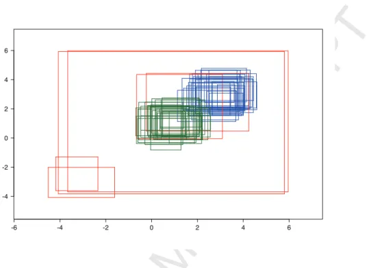
-6 -4 -2 0 2 4 6 -4 -2 0 2 4 6
Figure 3: Example of randomly generated data set (casesep= 2,n= 60,low, cen). For each observation, reported are the supports of the two fuzzy variables. The black, red and blue rectangles refer to the outliers and to the observations belonging to Cluster 1 and 2, respectively.
2sep, from which it is clear that their spreads were abnormal. For every level of every design variable, 10 data sets were randomly generated. An example of randomly generated data set is reported in Figure 3. Hence, 2 (numbers of clusters, k = 2,3) × 2 (numbers of variables, p = 2,8) × 4 (data sizes, n = 60,120,180,240) × 2 (cluster structures, cen or spr) × 2 (levels of separation between clusters, sep = 1,2) × 2 (percentages of contamination, low orhigh) × 10 (replications) = 1280 LR fuzzy data sets were randomly generated during the simulation experiment. All these data sets were analyzed by PFkM-F, FkM-F, PkM-F and C-PkM-F setting k = 2 ork= 3 according to the known in advance number of clusters. Five random starts were used for PFkM-F and FkM-F. The optimal solution of FkM-F was the only one (rational) starting point for the PkM-F and C-PkM-F algorithms.
Except for k, the parameters of the PFkM-F algorithm were determined using the selection procedure proposed in Section 5.2. The possible values of
m and η ranged from 1.5 to 2.5 with step equal to 0.25. The parameters a
and b took scores from 0.5 to 5 with step equal to 0.5. In order to guarantee that the values of aand b were not “too far”, we imposed that the difference between a and b in absolute value was not higher than 2. For instance, if
a = 1.5, then the possible values of b were {0.5,1,1.5,2,2.5,3,3.5}. More-over, in order to avoid solutions with a large number of observations having low degrees of typicality, i.e., observations recognized as outliers, we consid-ered the following rule. We skipped solutions, i.e., we did not compute the
XBP F−F index, when the clustering method recognized at least one half of the observations as outliers. The same grid search was considered for the se-lection of min FkM-F and ofη in PkM-F and C-PkF-F. The optimal values ofmfor FkM-F and ηfor PkM-F were determined in such a way to minimize
XBP F−F. This was applied setting a = 1 and b = 0 for FkM-F and a = 0 and b = 1 for PkM-F. Note that for PkM-F and C-PkM-F we adopted the previously described rule for skipping meaningless solutions. Nonetheless, if, for a certain data set, feasible PkM-F or C-PkM-F solutions were not found, then the rule was ignored.
6.1.1. Results
First of all, the selection procedure for PFkM-F proposed in Section 5.2 gave the following average values computed using all the 1280 data sets:
m = 1.63, η= 1.72, a= 3.16 andb = 1.69. Thus, the values ofmandηwere almost equal on average, whereas the selection procedure tended to choose a value of a higher than the one of b. For FkM-F the average value of m was 1.67, for C-PkM-F and PkM-F the ones ofηwere 1.99 and 2.32, respectively. In order to evaluate how the clustering methods worked, we observed their ability to estimate properly the centroids and to assign the non-outliers and the outliers to the clusters with high or low degrees of sharing or typicality, respectively. To assess how well every method recovered the true centroids we computed the REC measure based on the sum of the squared dissimilarities of the centers and the spreads between all the true and estimated centroids:
REC = k g=1 d2 hC1 g ,h C1 g T +d2 hC2 g ,h C2 g T +d2 hLg,hLgT +d2 hRg,hRgT ,(32)
where the superscript ‘T’ refers to the matrices of the centers and the spreads for the true centroids determined using the non-outliers, i.e., computing the average values of the observations belonging to every cluster. To analyze the
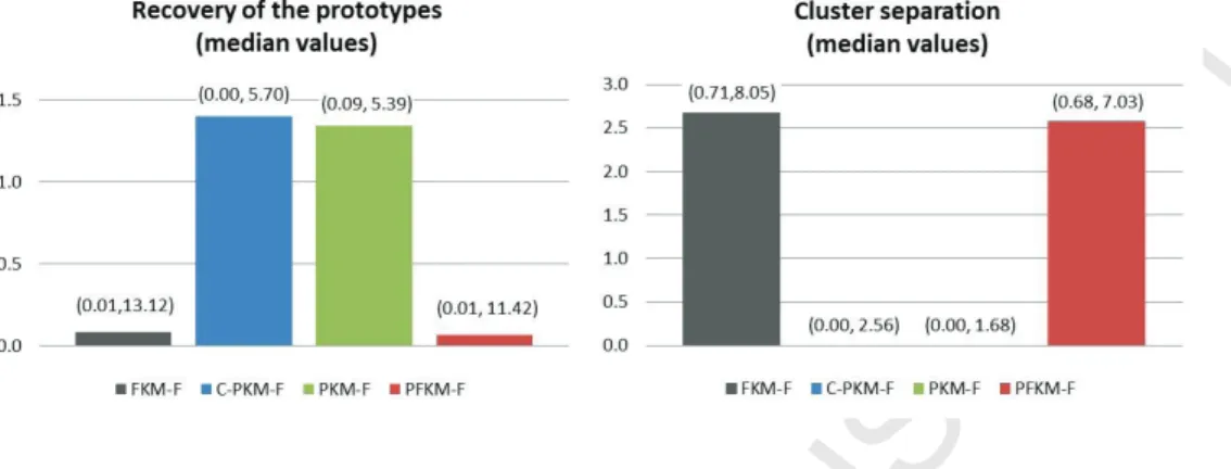
Figure 4: Median values and 10th and 90thpercentiles (within parentheses) of REC and
SEP.
level of separation between centroids, we computed theSEP measure, based on the minimum sum of the squared dissimilarities of the centers and the spreads between pairs of centroids:
SEP = min g,g(g=g) d2hC1 g ,h C1 g +d2hC2 g ,h C2 g +d2hLg,hLg +d2hRg,hRg .(33)
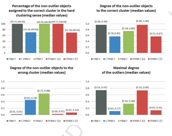
Figure 4 displays the median values and the 10th and 90th percentiles of (32) and (33) for the four methods. To investigate how well the four methods assigned the observations to the clusters we studied the percentage of non-outliers assigned to the correct cluster in the hard clustering sense, i.e., with degrees of sharing or typicality higher than 0.5. With regard to the non-outliers we also checked the degrees of sharing or typicality to the correct and wrong cluster. Finally, we analyzed the maximal degree of the outliers. The median values and the 10thand 90thpercentiles of the previous quantities are reported in Figure 5.
By inspecting Figure 4 some comparative assessments about how the methods recovered the prototypes can be given. The methods based on the fuzzy approach performed better than those based on the possibilistic one (REC values reported in the left side of Figure 4). This can be motivated by observing the medianSEP values (right side of Figure 4) from which we can see the tendency of the possibilistic methods to produce coincident clusters. Note that the percentage of occurrences of trivial solutions was 72.27% and 79.61% for C-PkM-F and PkM-F, respectively. A good compromise was achieved by PFkM-F that worked well by exploiting the potentialities of
Figure 5: Median values and 10thand 90thpercentiles (within parentheses) of percentages of outliers assigned (hard clustering sense) to the correct cluster, degrees of non-outliers assigned to the correct and wrong cluster and maximal degrees of non-outliers.
the possibilistic and fuzzy approaches, namely, it estimated the prototypes reasonably well and avoided coincident clusters (no trivial PFkM-F solutions were registered during the entire simulation study).
By inspecting Figure 5, we can see that the fuzzy membership degree information (the matricesU from FkM-F and PFkM-F) was more insightful than the possibilistic membership degree information (the matrices T from C-PkM-F, PkM-F and PFkM-F) with respect to the non-outliers, but was not helpful when dealing with contaminated data. In fact, non-outliers were almost always assigned to the correct cluster (top left side of Figure 5) with high (median equal to 0.97) fuzzy membership degrees (top right side of Figure 5) by applying FkM-F and PFkM-F (considering U). A good per-formance was also observed for PkM-F. However, by looking at the low and left side of the figure, we can observe that PkM-F also tended to give high
degrees of typicality to the wrong cluster. This occurred because PkM-F frequently produced coincident clusters and, hence, high degrees of typical-ity to all the clusters. The fuzzy membership degrees were not informative to recognize the outliers (bottom right side of Figure 5). In fact, by con-sidering the fuzzy membership degree matrix U from FkM-F, we could not assess whether outliers were present in the data. This was not the case when we considered the possibilistic membership degrees. In fact, C-PkM-F and PkM-F assigned the outliers to the clusters with median degrees of typicality lower than 0.5. The above comments on fuzzy and possibilistic membership degrees jointly hold for PFkM-F. This allows us to highlight the complemen-tary information provided by U and T. More specifically, on the one hand, the degrees of typicality (in T) allowed us to properly discover the presence of outliers. On the other hand, the degrees of sharing (in U) allowed us to properly discover the fuzzy cluster structure.
6.1.2. Computational issues
We investigated some computational issues related to the PFkM-F algo-rithm for fixed values of k, a, b, m and η (without taking into account the computational time of the parameter selection procedure proposed in Section 5.2). The computational complexity of PFkM-F has the same order of mag-nitude as FkM and, in particular, it is linear with respect to the number of observations, O(n). We studied it in practice together with the tendency of the algorithm to hit local optima. The former point was analyzed by observ-ing the computation time in seconds. Note that the simulation study was carried out on a personal computer with 2.80 GHz processor and 16.00 GB RAM and the convergence criterion was 10−5. The risk of local optima was assessed by recording, for each data set, the percentage of times in which the function value was less than 0.1% bigger than that of the purported global optimum (PGO). The PGO was defined as the best estimate of the global optimum, i.e., for each data set, the best solution out of five runs of the PFkM-F. The results concerning computation time and risk of local optima referred to the runs of PFkM-F setting the parameters according to the selec-tion procedure of Secselec-tion 5.2. The average computaselec-tion time of the PFkM-F algorithm was 0.39s. It mainly depended on the number of observations (the average computation times were equal to 0.14s and 0.62s when n = 60 and
n = 240, respectively), the number of clusters (0.24s when k = 2 and 0.54s when k = 3), the number of variables (0.26s when p = 2 and 0.51s when
contami-nation and 0.51s for the high one). The registered computation times were almost always lower than 1.00s (93.84% of times) and the maximum one was lower than 10.00s.
The average percentage of times in which the PGO was attained was 59.97%. We observed that the PFkM-F algorithm was more prone to hit the PGO when k = 2, when the clusters were distinguished by the spreads (spr case) and when the level of contamination was low (low case): in such cases the percentages of attaining the PGO were 70.28%, 72.06% and 73.19%, respectively. Therefore, more than one random start is suggested to reduce the risk of local optima. In particular, the use of five random starts appears to be appropriate.
6.2. Real data
6.2.1. Sensory profiling Gamonedo cheese data
The first application to real data was an example in sensory analysis. The quality of a specific kind of cheese from Asturias (Spain), named Ga-monedo blue cheese, has been investigated by the LILA institute for obtaining the Protected Designation of Origin (PDO) [42]. This was done by taking into account the subjective perceptions of experts about n = 42 Gamonedo cheeses made by different producers with respect to p = 11 characteristics: shape, rind, texture aspect, smell intensity, smell quality, texture hardness, crispness, flavour intensity, flavour quality, aftertaste, global quality. In par-ticular, for each cheese the expert was invited to express her/his perception using a graduate scale ranging from 0% (lowest quality) to 100% (highest quality). We believed that these perceptions did not allow a precise repre-sentation. Hence, according to the ontic treatment, they were managed by fuzzy data seen as whole entities. Specifically, the perception of each char-acteristic was represented by means of a trapezoidal fuzzy number whose 0-level was the set of values that were compatible with the opinion of the taster at some extent and the 1-level was the set of values that were fully compatible with her/his opinion. Finally, the trapezoidal fuzzy number was obtained by linearly interpolating these two levels. The assessments made by one of the experts were analyzed by PFkM-F 1. The optimal parameters were found in connection with the minimum of XBP F−F (see, Figure 6). We got k= 2, m = 1.5, η= 2, a= 3 and b= 1.
Number of clusters XB PF F 2 3 4 5 6 0.0 0.5 1.0 1.5 2.0 2.5 3.0 3.5
Figure 6: Values of XBP F−F for number of cluster k from 2 to 6, related to the sensory profiling Gamonedo cheese data.
In order to visualize the results, in Figure 7 we displayed the cheeses and the centroids onto the plane found by applying Principal Component Anal-ysis for fuzzy data [43]. First of all it was interesting to discover that the first component (x-axis) was mainly related to smell intensity, smell qual-ity, flavour intensqual-ity, flavour qualqual-ity, aftertaste and global qualqual-ity, hence this component reflected the smell and taste likings, closely related to the global quality. Component 2 (y-axis) depended on shape, rind and texture aspect and, thus, was interpreted as the sight liking. By observing the centroids, the two clusters distinguished ‘high quality Gamonedo cheeses’ (Cluster 1) and ‘low quality Gamonedo cheeses’ (Cluster 2). In the hard clustering sense, the fuzzy partition was composed by clusters of size 23 (Cluster 1) and 19 (Clus-ter 2). Some cheeses (denoted by dashed line rectangles) shared their fuzzy membership degrees between the two clusters. In fact, they were assigned to Cluster 1 with membership degrees lower than 0.70. Hence, they had in-termediate values between the two clusters. To assess how far these cheeses were from the centroids, the degrees of typicality in the matrix Twere
stud-Component 1
Component 2
Figure 7: Plot of the first two components of the sensory profiling Gamonedo cheese data. The blue rectangles refer to cheeses assigned to Cluster 1 and the green ones to those assigned to Cluster 2; the solid or dashed lines denote cheeses assigned to the clusters with membership degree≥0.70 or in the interval in the interval (0.50,0.70), respectively; the dotted line denotes the anomalous cheeses characterized by low maximal degrees of typicality; the bold solid line denotes the centroids.
ied. Among others, an interesting finding concerned the cheese represented by a dot line rectangle. It was clearly assigned to Cluster 2 (with degree of sharing equal to 0.88), but the corresponding degree of typicality was very low (0.16). This showed that the involved cheese was very far from both the clusters. It was assigned to Cluster 2 because it was extremely far from the centroid of Cluster 1. On the basis of the cluster interpretation, we concluded that such a cheese was an outlier because it was definitely not appreciated by the expert, i.e. its scores were noticeably lower than those pertaining to the other cheeses.
6.2.2. Temperature data
The data referred to the monthly temperatures in Celsius degrees of a set of geographical units in Italy. We assumed that the temperature of a
Number of clusters XB PF F 2 3 4 5 6 0.0 0.5 1.0
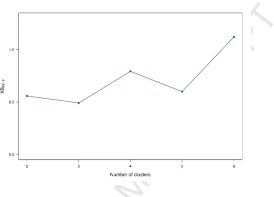
Figure 8: Values ofXBP F−F for number of cluster kfrom 2 to 6, related to the monthly temperature data.
certain geographical unit is an intrinsically fuzzy datum due to size of the area. Thus, the imprecision of the data was considered in the ontic sense. For every geographical unit (n= 162) and every month (p= 12 the information was represented by a triangular fuzzy number2.
The use of the PFkM-F clustering algorithm aimed at discovering some common patterns among the geographical units and the existence of anoma-lous geographical units. The optimal parameters were found according to
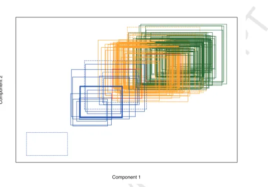
XBP F−F (Figure 8). We gotk = 3, m = 1.75, η = 2, a= 4.5 and b= 2.5. The three clusters highlighted the presence of three levels of temperature: hot, warm and cold. In the hard clustering sense, according to the degrees of sharing in U, such a fuzzy partition was composed by clusters of size 71, 76 and 13, respectively. A summary of the PFkM-F results is displayed in Figure 9 where we plotted the geographical units and the centroids onto the planes spanned by the first two principal components [43].
Component 1
Component 2
Figure 9: Plot of the first two components of the temperature data. The green rectangles refer to geographical units assigned to Cluster 1, the orange ones to those assigned to Cluster 2 and the blue ones to those assigned to Cluster 3; the solid or dashed lines denote geographical units assigned to the clusters with membership degrees ≥ 0.70 or in the interval (0.50,0.70), respectively; the red dotted rectangles denote geographical units not assigned to the clusters in the hard clustering sense (degrees of sharing<0.50); the green or blue dotted lines denote anomalous geographical units assigned to the clusters (degrees of sharing≥0.50) and characterized by low maximal degrees of typicality; the bold solid line denotes the centroids.
The locations of the centroids was consistent with the cluster interpreta-tion taking into account that Components 1 and 2 reflected the wintertime and summertime temperatures, respectively. From the top right side to the bottom left side the centroids of Clusters 1 (green solid line rectangle), 2 (or-ange solid line rectangle) and 3 (blue solid line rectangle) are ordered. Apart from some exceptions, the first two clusters discriminated the geographi-cal units with respect to their positions. In detail, Clusters 1 and 2 were composed by geographical units from Southern and Northern-Central and Italy, respectively. Instead, mountain geographical units belonged to Cluster 3. Therefore, this cluster of smaller size had the merit of highlighting the unique features of the geographical units characterized by high altitude.
The majority of the geographical units were assigned to the clusters with high (≥0.70) degrees of sharing (solid line rectangles of different colors ac-cording to the cluster memberships). A small percentage (about 13%), de-noted by dashed line rectangles, was assigned to the clusters with membership degrees lower than 0.70 (and higher than 0.50). Only two geographical units, Firenzuola and Monte Calamita from Tuscany (represented by black solid line rectangles), were not assigned to the clusters with membership degrees greater than 0.50. This occurred because these units had intermediate val-ues between two clusters. In particular, Firenzuola shared the features of Clusters 1 and 2 and Monte Calamita those of Clusters 2 and 3.
In order to detect anomalous geographical units, we inspected the typ-icality matrix T. We discovered at least two outliers (Plateau Rosa and Lampedusa) displayed by dotted line rectangles. The temperatures of these geographical units were extremely far from those of all the centroids. Plateau Rosa (rectangle in the bottom left side) was assigned to Cluster 3 with de-gree of sharing equal to 0.76, but the corresponding dede-gree of typicality is 0.01. It is a mountain geographical units located in front of the Matterhorn mountain with altitude higher than 3000 meters. The registered tempera-tures were much colder than those of the centroid of Cluster 3. The opposite comment held for Lampedusa, the southernmost part of Italy, with respect to Cluster 1 (degrees of sharing and typicality to Cluster 1 equal to 0.83 and 0.09, respectively). The associated rectangle (in the top right of the figure) had the center farthest to the right. In fact, Lampedusa had extremely hot temperatures, especially in the wintertime.
7. Concluding remarks
In this paper we have developed some robust clustering methods for non-precise information. First we have proposed a fully possibilistic version of thek-means clustering method for LR fuzzy data (PkM-F) where, differently from the fuzzy approach, the sum of the membership degrees of an obser-vation to all the clusters is no longer required to be equal to one. In this respect, the possibilistic membership degrees can be interpreted as degrees of typicality, rather than as degrees of sharing as is the case for the fuzzy ap-proach. Although PkM-F should be not sensitive to outliers, it has a major limitation, namely coincident clusters may occur. To overcome this problem, a second approach has been proposed. It consists in hybridizing the fuzzy and possibilistic approaches to clustering, exploiting the benefits of both the
approaches (i.e., to extract information about the fuzzy partition and the typicality of the observations) and avoiding their limitations (i.e., disruptive effect of outliers and coincident cluster problem). We have referred to this method as possibilistic fuzzy k-means clustering method for LR fuzzy data (PFkM-F). Some parameters must be set before running the PFkM-F. A selection procedure for choosing good values for these parameters has been proposed. It is based on a novel cluster validity index for hybrid clustering methods such as PFkM-F. We have checked the adequacy of PFkM-F by means of simulation and real-case studies. This has been done by comparing the performance of PFkM-F with the ones of other related clustering meth-ods for fuzzy data. We have found that PFkM-F worked in a satisfactory way also in comparison with its competitors.
On the basis of these good results, we indicate at least three perspectives of research: to speed up the selection procedure for the PFkM-F parameters by using, for instance, a line search strategy or a Pareto analysis; to generalize to the full LR family the possibilistic clustering method proposed in [23]; to develop biclustering methods for non-fuzzy and/or fuzzy data according to the fuzzy and possibilistic approaches.
Acknowledgements
We are grateful to anonymous reviewers for their critical and valuable comments on the manuscript. The research in this paper has been partially supported by the Italian Ministry of Education, University and Research (MIUR) grant “Mixture and latent variable models for causal inference and analysis of socio-economic data” (FIRB 2012). The first author is also grate-ful to the COST Action IC1408 “Computationally-intensive methods for the robust analysis of non-standard data”.
[1] Zadeh, L.A., 1965. Fuzzy sets. Inf. Control 8, 338–353.
[2] Coppi, R., 2008, Management of uncertainty in Statistical Reasoning: The case of Regression Analysis. Int. J. Approx. Reason. 47, 284–305. [3] Blanco-Fern´andez, A., Casals, M.R., Colubi, A., Corral, N.,
Garc´ıa-B´arzana, M., Gil, M.A., Gonz´alez-Rodr´ıguez, G., L´opez, M.T., Lubiano, M.A., Montenegro, M., Ramos-Guajardo, A.B., de la Rosa de S´aa, S., Sinova, B., 2014. A distance-based statistical analysis of fuzzy number-valued data. Int. J. Approx. Reason. 55, 1487–1501.
[4] Couso, I., Dubois, D., 2014. Statistical reasoning with set-valued infor-mation: ontic vs. epistemic views, Int. J. Approx. Reason. 55, 1502–1518. [5] Colubi, A., Gonz´alez-Rodr´ıguez, G., 2015. Fuzziness in data analysis:
towards accuracy and robustness, Fuzzy Sets Syst. 281, 260–271.
[6] Hariz, S.B., Elouedi, Z., Mellouli, K., 2006. Clustering approach using belief function theory. In: Euzenat, J., Domingue, J. (eds.) Artificial Intel-ligence: Methodology, Systems, and Applications, Springer, pp.162–171. [7] Quost, B., Denoeux, T., 2010. Clustering fuzzy data using the fuzzy EM
algorithm. In: Deshpande, A., Hunter, A. (eds.) Proceedings of the 4th In-ternational Conference on Scalable Uncertainty Management, SUM’2010, Toulouse, France, Springer-Verlag, pp.333–346.
[8] Quost, B., Denoeux, T., 2016. Clustering and classification of fuzzy data using the fuzzy EM algorithm. Fuzzy Sets Syst. 286 134–156.
[9] Sato, M., Sato, Y., 1995. Fuzzy clustering model for fuzzy data. FUZZ-IEEE’95, 2123–2128.
[10] Hathaway, R.J., Bezdek, J.C., Pedrycz, W., 1996. A parametric model for fusing heterogeneous fuzzy data. IEEE Trans. Fuzzy Syst. 4, 1277–1282. [11] Yang, M.S., Ko, C.H., 1996. On a class of fuzzy c-numbers clustering
procedures for fuzzy data. Fuzzy Sets Syst. 84, 49–60.
[12] Pedrycz, W., Bezdek, J.C., Hathaway, R.J., Rogers, G.W., 1998. Two nonparametric models for fusing heterogeneous fuzzy data. IEEE Trans. Fuzzy Syst. 6, 411–425.
[13] Takata, O., Miyamoto, S., Umayahara, K., 1998. Clustering of data with uncertainties using Hausdorff distance. Proceedings of the IEEE Interna-tional Conference on Intelligence Processing Systems, 67–71.
[14] Yang, M.-S., Liu, H.-H., 1999. Fuzzy clustering procedures for conical fuzzy vector data. Fuzzy Sets Syst. 106 189–200.
[15] Takata, O., Miyamoto, S., Umayahara, K., 2001. Fuzzy clustering of data with uncertainties using minimum and maximum distances based on L1 metric. Proceedings of the Joint 9th IFSA World Congress and 20th NAFIPS International Conference, 2511–2516.
[16] Auephanwiriyakul, S., Keller, J.M., 2002. Analysis and efficient imple-mentation of a linguistic fuzzy c-means. IEEE Trans. Fuzzy Syst. 10, 563– 582.
[17] Coppi, R., D’Urso, P., 2003. Three-way fuzzy clustering models for LR fuzzy time trajectories. Comput. Stat. Data Anal. 43 149–177.
[18] Yang, M.-S., Hwang, P.-Y., Chen, D.-H., 2004. Fuzzy clustering algo-rithms for mixed feature variables, Fuzzy Sets Syst. 141, 301–317.
[19] D’Urso, P., Giordani, P., 2006. A weighted fuzzy c-means clustering model for fuzzy data. Comput. Stat. Data Anal. 50 1496–1523.
[20] Hung, W.-L., Yang, M.-S., 2005. Fuzzy clustering on LR-type fuzzy numbers with an application in Taiwanese tea evaluation fuzzy clustering on LR-type fuzzy numbers with an application in Taiwanese tea evaluation. Fuzzy Sets Syst. 150 561–577.
[21] Zarandi, M.H.F., Razaee, Z.S., 2011. A fuzzy clustering model for fuzzy data with outliers. Int. J. Fuzzy Syst. Appl. 1, 29–42.
[22] Coppi, R., D’Urso, P., Giordani, P., 2012. Fuzzy and possibilistic clus-tering for fuzzy data. Comput. Stat. Data Anal. 56, 915–927.
[23] Ferraro, M.B., Giordani, P., 2013. On possibilistic clustering with repul-sion constraints for imprecise data. Inf. Sci. 245, 63–75.
[24] D’Urso, P., De Giovanni, L., 2014. Robust clustering of imprecise data. Chemom. Intell. Lab. Syst. 136, 58–80.
[25] Hung, W.L., Yang, M.-S., 2015. Automatic clustering algorithm for fuzzy data. J. Appl. Stat. 42, 1503–1518.
[26] Banerjee, A., Dav´e, R.N., 2012. Robust clustering. WIREs Data Mining Knowl. Discov. 2, 29–59.
[27] Krishnapuram, R., Joshi, A., Nasraoui, O., Yi, L., 2001. Low-complexity fuzzy relational clustering algorithms for web mining. IEEE Trans. Fuzzy Syst. 9, 595–607.
[28] Garc´ıa-Escudero, L., Gordaliza, A., 1999. Robustness properties of k -means and trimmed kmeans. J. Am. Stat. Assoc. 94, 956-969.
[29] Kim, J., Krishnapuram, R., Dav´e, R., 1996. Application of the least trimmed squares technique to prototype based clustering. Pattern Recogn. Lett. 17, 633–641.
[30] Dav´e, R.N., 1991. Characterization and detection of noise in clustering. Pattern Recogn. Lett. 12, 657–664.
[31] Jajuga, K., 2001. L1-norm based fuzzy clustering. Fuzzy Sets Syst. 39, 43–50.
[32] Wu, K.L., Yang, M.S., 2002. Alternative c-means clustering algorithms. Pattern Recogn. 35, 2267–2278.
[33] Krishnapuram, G.L., Keller, J.M., 1993. A possibilistic approach to clus-tering. IEEE Trans. Fuzzy Syst. 1, 98–110.
[34] Barni, M., Cappellini, V., Mecocci, A., 1996. Comments on ‘a possibilis-tic approach to clustering’. IEEE Trans. Fuzzy Syst. 4, 393–396.
[35] Pal, N.R., Pal, K., Bezdek, J.C., 1997. A Mixed c-Means Clustering Model. FUZZ-IEEE’97, 11–21.
[36] Pal, N.R., Pal, K., Keller, J.M., Bezdek, J.C., 2005. A possibilistic fuzzy
c-means clustering algorithm. IEEE Trans. Fuzzy Syst. 13, 517–530. [37] Bezdek, J.C., 1981. Pattern recognition with fuzzy objective function
algorithm. Plenum Press, New York.
[38] Xie, X.L., Beni, G., 1991. A validity measure for fuzzy clustering. IEEE Trans. Pattern Anal. 13, 841–846.
[39] Yang, M.S., Wu, K.L., 2006. Unsupervised possibilistic clustering. Pat-tern Recogn. 39, 5–21.
[40] Campello, R.J.G.B., Hruschka, E.R, 2006. A fuzzy extension of the sil-houette width criterion for cluster analysis. Fuzzy Sets Syst. 157, 2858– 2875.
[41] Rousseeuw, P.J., 1987. Silhouettes: a graphical aid to the interpretation and validation of cluster analysis. J. Comput. Appl. Math. 20, 53–65.