Efficient Multi-modal Geometric Mean Metric Learning
Jianqing Lianga, Qinghua Hua,, Pengfei Zhua, Wenwu Wangb
aSchool of Computer Science and Technology, Tianjin Univerity, Tianjin, China
bDepartment of Electronic Engineering, University of Surrey, United Kingdom
Abstract
With the fast development of information acquisition, there is a rapid growth of modality data, e.g., text, audio, image and even video, in fields of health care, multi-media retrieval and scientific research. Confronted with the challenges of clustering, classification or regression with multi-modality information, it is essential to effective-ly measure the distance or similarity between objects described with heterogeneous features. Metric learning, aimed at finding a task-oriented distance function, is a hot topic in machine learning. However, most existing algorithms lack efficiency for high-dimensional multi-modality tasks. In this work, we develop an effective and efficient metric learning algorithm for multi-modality data, i.e., Efficient Multi-modal Geomet-ric Mean MetGeomet-ric Learning (EMGMML). The proposed algorithm learns a distinctive distance metric for each view by minimizing the distance between similar pairs while maximizing the distance between dissimilar pairs. To avoid overfitting, the optimiza-tion objective is regularized by symmetrized LogDet divergence. EMGMML is very efficient in that there is a closed-form solution for each distance metric. Experiment re-sults show that the proposed algorithm outperforms the state-of-the-art metric learning methods in terms of both accuracy and efficiency.
Keywords: Metric learning; multi-modality; efficiency; geometric mean.
Email addresses:[email protected](Jianqing Liang),[email protected]
1. Introduction
Multi-modality data are booming with the ubiquitous usage of digital devices and social network. In multi-media retrieval, there exists a large variety of data, e.g., text, audio, image, video, etc., on the website. In biometric recognition, a person can be identified by retina, face, iris, signature, fingerprint, or palmprint [1, 2, 3, 4, 5]. For
5
face recognition, a face image may be captured by cell phones, near-infrared cameras or depth cameras [6, 7, 8, 9, 10, 11, 12, 13]. An object is usually described by differ-ent modalities with complemdiffer-entary information in many computer vision and pattern recognition tasks.
Learning a task-driven metric from massive multi-modality data automatically is
10
meaningful to diverse applications such as computer vision, bioinformatics and infor-mation retrieval. Metric learning, which aims to train an appropriate measure from data, has provoked wide interests over the past decade. A large number of approaches have been proposed, most of which intend to learn a Mahalanobis-like metric. Gen-erally, according to the optimality of the solution, metric learning can be categorized
15
into global methods and local methods. Global methods can be regarded as learning a linear geometric transformation over the input space [14, 15, 16, 17]. While the sim-plicity promotes their wide application, the global metrics still suffer from the curse of dimensionality. Compared with global metrics, local metrics have been shown to be able to flexibly capture geometric variations across different feature spaces [18, 19, 20].
20
However, a major drawback of local metric learning is that it may lead to overfitting [21]. In addition, they are generally confronted with high computational cost.
Despite the large amount of work on single modality, learning metrics for mul-tiple modalities still remains largely unexploited [22]. Since single metrics ignore consensus&complementarity properties between different modalities, it may fail in
25
multi-modal learning. Under such circumstance, multiple kernel techniques, which map the data to high-dimensional feature spaces with a set of nonlinear kernel matri-ces, have been introduced to address these issues [7, 23, 24]. To our best knowledge, McFee and Lanckriet [23] first utilized multiple kernel learning technique to integrate heterogeneous modalities into a single, unified similarity space. In their work, an
timal ensemble of kernel transformations is learned. Unfortunately, it is not applicable to large-scale tasks due to the expensive computational costs. In [24], Lu et al pro-posed a weighted kernel embedding technique for metric learning, which is shown to be effective in combining multiple features. Recently, Lu et al [7] exploited statistics information to represent image sets and developed a a localized multi-kernel metric
35
learning (LMKML) method. While state-of-the-art performance has been achieved, it still remains to explore an efficient strategy to improve the speed. Generally speaking, although multiple kernel learning may capture the complex data structure and avoid the curse of dimensionality , the time-consuming process in terms of parameter adjustment limits its scalability in large-scale tasks.
40
A distance metric learning algorithm is evaluated in terms of both accuracy and efficiency. Although these aforementioned methods significantly surpass the state-of-the-arts, the high time complexity limits their scalability in practical applications, especially in handling multi-modality data. As time cost as well as the memory re-quirement dramatically increases when dealing with large-scale data represented with
45
high-dimensional multiple modalities, how to develop an effective and efficient metric learning method has become a hot topic. To solve the problem, online learning tech-niques have been considered [25, 26]. In [25], a novel Online Multiple Kernel Similar-ity (OMKS) learning framework is proposed to learn a flexible proximSimilar-ity function with multiple kernels. In [26], an online multi-modal distance metric learning (OMDML)
50
scheme is put forward, which aims at learning distinctive metrics in individual modal-ity space and the weights for combining different modalities via a joint formulation. While online approaches are more scalable compared with the batch processing tech-niques, they are more likely to suffer from high computational cost in projections in that iteration process involves gradient descent method.
55
As the iterative gradient descent or eigenvalue decomposition is used in solving the optimization problem, most of metric learning algorithms are computationally ex-pensive. Remarkably, Zadeh et al [27] developed Geometric Mean Metric Learning (GMML), which formulates metric learning as an unconstrained smooth and strictly convex optimization problem. GMML is very efficient for large-scale tasks in that it
60
common-ness and individuality should be made good use of to improve the discrimination ability of the learned metrics.
In this paper, we develop a novel Efficient Multi-modal Geometric Mean Met-ric Learning (EMGMML) framework to handle data with multiple modalities, which
65
means multiple visual features extracted from media objects. EMGMML learns the metrics for multiple features in a joint optimization problem by pulling similar pairs close whereas pushing dissimilar pairs away. To explore the complementarities among different modalities, the learned metrics for different modalities are required to be close to a common prior metric by symmetrized LogDet divergence. Meanwhile, to highlight
70
the difference of multi-modalities, we assign a weight to each modality. Specifically, each metric connected with the modality can be solved in a closed form solution. Then, the metric learning problem can be converted into a quadratic programming in terms of weights. Compared with existing metric learning approaches, EMGMML is highly s-calable and efficient due to exemption from kernel mapping and solving a semi-definite
75
programming problem. Empirical results on benchmark datasets with hundreds of di-mensions verify that multiple weighted metrics obtained by our algorithm complete prominent performance boost in terms of visual search.
The remainder of this paper is organized as follows. Section 2 briefly reviews the GMML algorithm in [27]. In Section 3, we introduce our proposed EMGMML
80
algorithm for high-dimensional multi-modal data. Section 4 analyzes experimental results on both qualitative and quantitative point of view. Section 5 concludes our study and gives an outlook for our future work.
2. Geometric Mean Metric Learning Model
In this section, we review Geometric Mean Metric Learning (GMML) [27]
algo-85
rithm.
2.1. Formulation
We aim to learn a Mahalanobis distance
wherex,x′∈Rdare data vectors andAis ad×dreal and symmetric positive definite (SPD) matrix to be solved. Constraints are provided in the form of positive / negative pairs
S:={(xi,xj)|xiandxjare in the same class}
D:={(xi,xj)|xiandxjare in different classes}.
The objective is to minimize the sum of distances between similar points with a matrixAand distances between dissimilar points withA−1
X (xi,xj)∈S dA(xi,xj) + X (xi,xj)∈D dA−1(xi,xj) (2)
The idea is that increasing the distancedA(x,y)between dissimilar pairs is e-quivalent to decreasingdA−1(x,y). The gradients ofdA anddA−1 are in opposite
directions, which can confirm the rationality of the idea.
90
Substituting the distance with traces, we get
min A≻0 X (xi,xj)∈S tr(A(xi−xj)(xi−xj)T)+ X (xi,xj)∈D tr(A−1(xi−xj)(xi−xj)T) (3)
We denote two crucial matrices S := P (xi,xj)∈S (xi−xj)(xi−xj)T, D:= P (xi,xj)∈D (xi−xj)(xi−xj)T, (4)
that are the similarity and dissimilarity matrices, respectively. Utilizing (4), we rewrite (3) as
min
A≻0h(A) := tr(AS) + tr(A
−1D). (5)
h(A)has some key properties such as geodesic convexity. Here are several con-cepts of geodesically convex functions.
Geodesic convexity is a generalization of linear convexity for sets and functions to nonlinear Riemannian manifolds [28]. The geodesic curve locally minimizes the Riemannian distances between two points. It connectingAandBon the SPD manifold is defined as
On the entire set of SPD, the definition of geodesically convex functions is given as follows [29]
Definition 1. A functionf on a geodesically convex subset of a Riemannian manifold isgeodesically convex, if for all pointsAandBin this set, it satisfies
f(A♯tB)≤tf(A) + (1−t)f(B), t∈[0,1].
If fort∈(0,1)the above inequality is strict, the function is called strictly
geodesi-95
cally convex.
Key properties ofh(A)is summarized as follows [27]
Theorem 1. The cost function h in (5) is both strictly convex and strictly geodesically convex on the SPD manifold.
2.2. Solution
100
According to the convexity of the objective function, we can obtain its global min-imum by setting the gradient as zero
∇h(A) =S−A−1DA−1= 0
Thus
ASA=D. (6)
Actually, the sole solution of (6) is the midpoint on the geodesic connectingS−1 andD[30], namely
A=S−1♯1/2D=S−1/2(S1/2DS1/2)1/2S−1/2.
Following the above definition, we know thatAis SPD.
While GMML obtains a closed-form solution, owing to the inverse matrix calcu-lation, it is still computationally expensive in handling high-dimensional multi-modal tasks. Furthermore, the performance may suffer due to the ignorance of correlation between different modalities. To solve this problem, we propose the framework of
105
3. Efficient Multi-modal Geometric Mean Metric Learning Model
In this section, we describe how to learn a geometric mean metric on multi-modality data.
3.1. Formulation
110
Given a set of samples X = [x1,x2, . . . ,xN], each sample xi is represented
withmmodalitiesx1i,x2i, . . . ,xmi , we aim at learning such a weighted Mahalanobis distance d{Ap,wp}mp=1(xi,xj) = m X p=1 wp(xpi −x p j) T Ap(xpi −x p j), (7)
wherexpi,xpj ∈Rdpare theith andjth point on thepth modality, respectively.w
pis a
weight that determines the importance of thepth modality in distance metric learning. Apis adp×dpreal and symmetric positive definite matrix to be learned for thepth
modality. Similarly, supervision information is given by sets of pairs in terms of each modality Sp:={(xpi,x p j)|x p i andx p
jare in the same class}
Dp:={(xpi,x p j)|x p i andx p
j are in different classes}.
Referring to the GMML algorithm, the objective can be
m X p=1 wp( X (xp i,x p j)∈Sp dAp(xpi,xpj) + X (xp i,x p j)∈Dp dA−1 p (x p i,x p j)) (8)
Rewriting the objective with traces, we turn (8) into
min {Ap}m p=1≻0 m X p=1 wp( X (xp i,x p j)∈Sp tr(Ap(xpi −x p j)(x p i −x p j) T) + X (xp i,x p j)∈Dp tr(A−p1(x p i −x p j)(x p i −x p j) T)) (9)
We now define the following two matricesSpandDp to represent similarity and
dissimilarity matrices for thepth modality Sp:= P (xp i,x p j)∈Sp (xpi −xpj)(xpi −xpj)T, Dp:= P (xp i,x p j)∈Dp (xpi −xpj)(xpi −xpj)T, (10)
Therefore, we can get the basic formulation of EMGMML min {Ap}m p=1≻0 h({Ap}mp=1) := m X p=1 wp(tr(ApSp) + tr(A−p1Dp)). (11)
As the matrixSpmay be near-singular or non-invertible, we add a regularizer to
the objective [27] min {Ap}m p=1≻0 m X p=1 wp(tr(ApSp) + tr(A−p1Dp)) +λ m X p=1 wpDsld(Ap,A0), (12)
whereA0is the prior metric andDsldis the symmetrized LogDet divergence
Dsld(Ap,A0) := tr(ApA0−1) + tr(A−p1A0)−2d, (13)
It is noteworthy that another variable iswp. To ensure the distance is positive, we
requirewp is negative. However, as the distance and divergence are both
non-negative, the objective obtains the minimum when eachwp equals 0. Since we hope
each modality can make their own contributions, mostwp should be positive. Thus,
we let the sum of wp be a constant. At this point, the objective becomes a linear
programming, which may cause most of them are near to zero. To avoid overfitting, we introduce a regularizer term ofwp. Ultimately, the regularized version of EMGMML
is min {Ap,wp}m p=1 m X p=1 wp(tr(ApSp) + tr(A−p1Dp)) +λ m X p=1 wpDsld(Ap,A0) +γ m X p=1 w2p, s.t. Ap≻0, p= 1,2, . . . , m wp≥0, p= 1,2, . . . , m m X p=1 wp = 1 (14) Letw= [w1, w2, . . . , wm]be am-dimensional vector, then
m P p=1 w2 pequalskwk22. 3.2. Solution
In the following, we develop an efficient optimization approach to solve (14). An alternative strategy is introduced in the solving procedure. Observing that the only
constraint of Ap is the positive definiteness, we consider to solve Ap at first. For
simplicity, we denote the function
L({Ap}mp=1) = m X p=1 wp(tr(ApSp) + tr(A−p1Dp)) +λ m X p=1 wpDsld(Ap,A0) (15)
The derivative ofLwith respect toApis
∂L ∂Ap =
wp(Sp−Ap−1DpA−p1) +λwp(A−01−Ap−1A0A−p1)
Setting it to zero leads to
wp= 0,or Sp−Ap−1DpA−p1+λ(A−01−Ap−1A0A−p1) = 0
However, ifwp = 0 holds for allp = 1,2, . . . , m, then we can not satisfy the
constraint m P p=1 wp= 1. Therefore Sp−A−p1DpAp−1+λ(A−01−A −1 p A0A−p1) = 0. (16)
We can obtain the solution
Ap= (Sp+λA−01)−1♯1/2(Dp+λA0), (17)
From the form of geometric mean, we may conclude thatApis SPD. Once theAp
is determined, the problem (14) is transformed to a quadratic programming onwp.
3.3. Weighted version
115
To generalize the scope of the solution, we propose the weighted EMGMML ob-jective with the optimalwp[30, 27]
min {Ap}m p=1≻0 ht({Ap}mp=1) := (1−t) m X p=1 wpδR2(Ap,Sp−1)+t m X p=1 wpδ2R(Ap,Dp), (18)
whereδRis the Riemannian distance on SPD matrices
δR(X,Y) :=klog(Y−1/2XY−1/2)kF f orX,Y ≻0,
As thewpis fixed and positive,SpandDpare known, the problem (18) is
equiva-lent to the followingmtasks:
min
Ap≻0 ht(Ap) = (1−t)δ 2
The unique solution is the weighted geometric mean
Ap=Sp−1♯tDp, (20)
Therefore, the regularized form of the solution is
Ap= (Sp+λA−01)−1♯t(Dp+λA0), t∈[0,1]
The algorithm is summarized in Algorithm 1.
Algorithm 1 The optimization of EMGMML Input:
{Sp}mp=1: set of similar pairs on each modality,
{Dp}mp=1: set of dissimilar pairs on each modality,
t: step length of geodesic,
λ: regularization parameter for metrics, γ: regularization parameter for weights, A0: prior knowledge
Output:
wp,Ap p= 1,2, . . . , m;
1: Compute the similarity and dissimilarity matrices forp= 1,2, . . . , m Sp= P (xp i,x p j)∈Sp (xpi −xpj)(xpi −xpj)T, Dp= P (xp i,x p j)∈Dp (xpi −xpj)(xpi −xpj)T
2: Return the distance matrix forp= 1,2, . . . , m Ap= (Sp+λA−01)−1♯t(Dp+λA0)
3: Return the weight forp= 1,2, . . . , m
TakeApinto (14) and solve the quadratic programming
3.4. Discussion
Let the dimension of thepth modality bedp,dmax = max
p∈[1,m]dp, then the total
dimension isd=
m
P
p=1
dp. The number of the pairs is denoted asT. The time cost of
GMML mainly lies in two parts: the computation of matricesS,Dand distance matrix
A. The time cost of the first part isO(T d2). The second part involves the matrix power
and multiplication, which costs bothO(d3). Therefore, the total time cost for GMML
should beO(T d2+d3). As for EMGMML, the first part costsO(mT d2
max)while the
second one isO(md3
max). The extra term induced by the quadratic programming is
O(m2). Asmis much smaller thand
max, thus, the time complexity of EMGMML is
125
O(mT d2max+md3max). From the above analysis, we know that as an extended version, EMGMML inherits the advantages of GMML in scalability. It is even more efficient in dealing with multi-modality high-dimensional data.
Overall, our proposed EMGMML framework projects multiple modalities onto dis-tinctive feature subspaces, and then exploits a weighted combination to integrate
cor-130
responding metrics. An alternative strategy is used for solving the joint objective of metrics as well as weights, which is showed to be both effective and efficient by em-pirical results in Section 4.
4. Experiments
In this section, we empirically analyze the performance of EMGMML. We first
135
describe the datasets and descriptors as well as the evaluation criterion. Then we e-laborate the compared methods and parameter setting and tuning. Finally, we compare EMGMML with state-of-the-arts in terms of effectiveness and efficiency on retrieval.
4.1. Datasets and Environment
We carry out the experiments on image datasets including Corel [15], ImageCLEF1,
140
Indoor2, Caltech2563 and Birds [31]. Some images are shown in Figure 1. For each dataset, several types of visual descriptors are exploited. Global features contain color histogram (256 dimensions for gray images and 768 dimensions for color images), GLCM coefficients (16 dimensions), LBP (59 dimensions) and GIST features (512 dimensions). Local features include the SIFT, dense-SIFT, SURF, Geometric Blur and
145
1http://imageclef.org/.
2http://web.mit.edu/torralba/www/indoor.html.
PHOG (680 dimensions) descriptors. All of these local descriptors are represented by Bag-of-Words (BOW) with vocabulary size as 200 except the last one. The basic information of these datasets is listed in Table 1. For image retrieval, we split the dataset into several parts: 50% for training (5% labeled and 45% unlabelled), 10% for validation, 10% for query, and the remaining 30% as pooling set. The experiment is
150
performed on a machine with 3.40 GHz Intel processor and 8 GB memory, and the Matlab software.
Table 1: Basic descriptions of datasets
Datasets # Classes # Dimensions # Samples
Corel 800 10 2835 800 ImageCLEF 10 2323 800 Indoor 10 2835 600 Caltech 10 10 2835 800 Birds 6 2835 600 Corel 5k 50 2835 5000
Figure 1: Several image examples in our experiments.
Referring to early literatures [32], we generate similar pairs by selecting two sam-ples from the same category and dissimilar pairs by picking up two samsam-ples from dis-tinct classes. The only difference is that we exploit all the samples from the training
set instead of random selection.
4.2. Evaluation Criterion
In this paper, we use mean average precision (MAP) to evaluate the performance of image retrieval. MAP is defined on the retrieved ranking list of queries. It is such a measurement of how the retrieved samples relate to the query. Given a query and itsR retrieved images, the Average Precision is defined as [33]
AP = 1 L R X r=1 prec(r)δ(r), (21)
whereLis the number of relevant samples in the retrieved set,prec(r)is the precision at therth position. δ(r)represents whether therth retrieved image is relevant to the query or not.δ(r) = 1when they are relevant and 0 otherwise. The MAP is computed
160
as the average AP of all the queries. We setRas the number of each class in the pooling set for small datasets, while we setRas 10 for large datasets like Corel 5k.
4.3. Comparison Methods
We compare the proposed algorithm with eight baseline methods.
• DCA. An efficient metric learning scheme which exploits both positive and
neg-165
ative constraints [15].
• LRML. A novel metric learning technique that integrates both labeled and
unla-belled data into an effective graph regularization framework [16].
• OASIS. A supervised online dual approach that learns a bilinear similarity
mea-sure [34].
170
• EMR. A scalable graph-based manifold ranking algorithm [35].
• DML-eig. An efficient eigenvalue optimization framework for metric learning
[36].
• OMKS. An efficient online metric learning algorithm which learns a flexible
nonlinear proximity function with multiple kernels for improving visual search
175
• SERAPH. An information-theoretic semi-supervised metric learning approach
that does not rely on the manifold assumption [17].
• GMML. A supervised metric learning method that is based on geometric
intu-ition and has a closed form solution [27].
180
To observe the effect of weights, we add a method called UGMML, which learns an optimal metric with GMML for each modality, and then uniformly combines all metrics. All of the distance metric learning approaches, except EMGMML, UGMML as well as OMKS, are performed on the concatenated feature vectors from different modalities.
185
4.4. Parameter Setting and Tuning
As for parameters, we only tune several key parameters on validation datasets for the best results and set all the others to default values. For GMML, we set the param-eterλ= 0.1. The prior matrixA0is set as the identity matrix [27]. The step lengtht
is adjusted in[0,1]with 0.1 step size. For EMGMML, The parameterγis tuned with
190
the ”grid-search” strategy from{10−4,10−3,10−2,10−1,1,10,102,103,104}. The
parameter settings ofλ,A0 andt are the same with GMML. Figure 2 gives the
in-fluence ofλon EMGMML. In fact,λcontrols the importance of the regularizer term with respect to each learned metricAp. It is clear that the performance on ImageCLEF
is sensitive to the choice of the parameterλ, while for other datasets the performance
195
remains relatively stable. For DML-eig, we tune the parameterk inkNN from 1 to the number of the labeled training images per class minus one [36]. As for LRML, we set the regularization parametersγs,γdas 1 and vary the parameterkofk-NN in 5-20
[16]. We set the number of the landmarks pickedpin EMR as 50. In OMKS, there are three parameters to be tuned, that is, the gaussian kernel parameterγ, discount weight
200
βas well as the trade-off parameterC[25].γis tuned from 0.01 to 0.1 with 0.01 inter-val.βis adjusted in the range of 0-1 with 0.01 interval andCis tuned in[0.001,0.01]
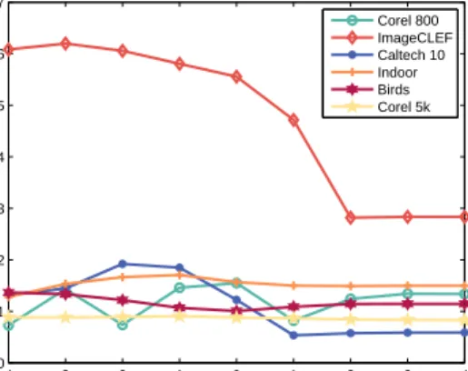
−4 −3 −2 −1 0 1 2 3 4 0 0.1 0.2 0.3 0.4 0.5 0.6 0.7 logλ mAP Corel 800 ImageCLEF Caltech 10 Indoor Birds Corel 5k
Figure 2: Retrieval performance versus logλon EMGMML. Other parameters are tuned to the best on the validation set.
4.5. Performance Comparisons
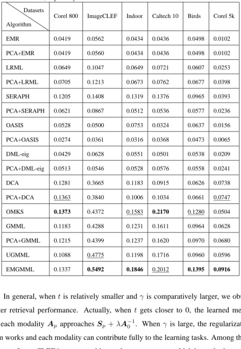
We report the MAP values for all the competing methods in Table 2. Methods with
205
’PCA’ as their prefixes indicate that we use PCA to reduce the dimension of original feature vectors to 200, and then perform retrieval with the corresponding metric. It can be seen that EMGMML consistently outperforms GMML in retrieval tasks. From top to down are unsupervised, semi-supervised and supervised methods. EMGMML improves the most on Indoor dataset with an increasement about 49.96%. On Corel 800
210
dataset, OMKS performance is equivalent to that of EMGMML, perhaps owing to the capability of non-linear metrics for capturing subtle differences. While UGMML may be inferior to GMML sometimes, for instance, on Corel 800, Indoor and Corel 5k, our EMGMML achieves a great improvement due to the learned reasonable weights. In our method, multiple metrics and weights are jointly performed to achieve the optimality,
215
thus yielding much better performance.
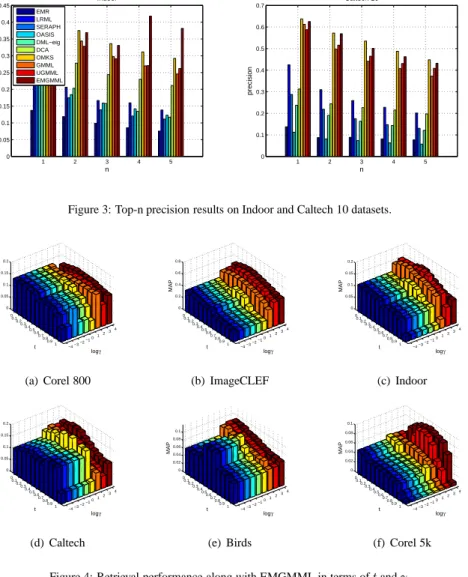
Figure 3 presents the top-n (n=1,2,. . . ,5) precision results on two datasets. It is clear that OMKS and EMGMML show comparative performance on Caltech 10. How-ever, EMGMML significantly outperforms all the other state-of-the-art metric learning algorithms on Indoor dataset.
220
Table 2: MAP of nine competing metrics for image retrieval. The best and the second best results are shown in bold and underlined, respectively
Algorithm Datasets
Corel 800 ImageCLEF Indoor Caltech 10 Birds Corel 5k
EMR 0.0419 0.0562 0.0434 0.0436 0.0498 0.0102 PCA+EMR 0.0419 0.0560 0.0434 0.0436 0.0498 0.0102 LRML 0.0649 0.1047 0.0649 0.0721 0.0607 0.0253 PCA+LRML 0.0705 0.1213 0.0673 0.0762 0.0677 0.0398 SERAPH 0.1205 0.1408 0.1319 0.1376 0.0965 0.0393 PCA+SERAPH 0.0621 0.0867 0.0512 0.0536 0.0577 0.0236 OASIS 0.0528 0.0500 0.0753 0.0324 0.0637 0.0156 PCA+OASIS 0.0274 0.0361 0.0316 0.0368 0.0473 0.0065 DML-eig 0.0429 0.0628 0.0551 0.0501 0.0538 0.0209 PCA+DML-eig 0.0513 0.0546 0.0528 0.0576 0.0558 0.0241 DCA 0.1281 0.3665 0.1183 0.0915 0.0626 0.0738 PCA+DCA 0.1363 0.3840 0.1006 0.1034 0.0661 0.0747 OMKS 0.1373 0.4372 0.1583 0.2170 0.1280 0.0504 GMML 0.1183 0.4288 0.1231 0.1611 0.0964 0.0628 PCA+GMML 0.1215 0.4399 0.1237 0.1620 0.0970 0.0680 UGMML 0.1088 0.4775 0.1198 0.1716 0.0960 0.0596 EMGMML 0.1337 0.5492 0.1846 0.2012 0.1395 0.0916
set. In general, whentis relatively smaller andγ is comparatively larger, we obtain better retrieval performance. Actually, whent gets closer to 0, the learned metric for each modalityAp approachesSp+λA−01. Whenγ is large, the regularization
term works and each modality can contribute fully to the learning tasks. Among these
225
datasets, ImageCLEF is more sensitive to these parameters, which is partly due to the fact that it is the only gray image dataset and thus much simpler.
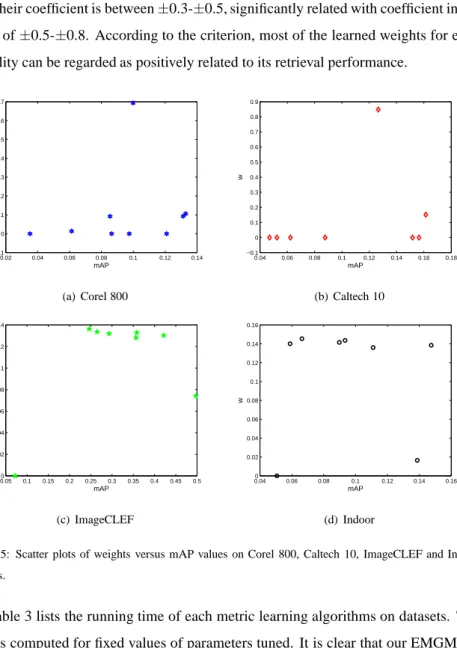
Our EMGMML method learns weights for each modality, which stands for its importance in learning metrics. Intuitively, the modality that has good performance
1 2 3 4 5 0 0.05 0.1 0.15 0.2 0.25 0.3 0.35 0.4 0.45 n precision Indoor EMR LRML SERAPH OASIS DML−eig DCA OMKS GMML UGMML EMGMML 1 2 3 4 5 0 0.1 0.2 0.3 0.4 0.5 0.6 0.7 n precision Caltech 10
Figure 3: Top-n precision results on Indoor and Caltech 10 datasets.
−4−3−2−10 1234 0 0.1 0.2 0.30.4 0.5 0.6 0.7 0.8 0.9 1 0 0.05 0.1 0.15 0.2 logγ t MAP (a) Corel 800 −4−3−2−10 1234 0 0.1 0.2 0.30.4 0.5 0.6 0.7 0.8 0.9 1 0 0.2 0.4 0.6 0.8 logγ t MAP (b) ImageCLEF −4−3−2−10 1234 0 0.1 0.2 0.30.4 0.5 0.6 0.7 0.8 0.9 1 0 0.05 0.1 0.15 0.2 logγ t MAP (c) Indoor −4−3 −2−101 234 0 0.1 0.2 0.3 0.4 0.5 0.60.7 0.8 0.9 1 0 0.05 0.1 0.15 0.2 logγ t MAP (d) Caltech −4−3 −2−101 234 0 0.1 0.2 0.3 0.4 0.5 0.60.7 0.8 0.9 1 0 0.02 0.04 0.06 0.08 0.1 logγ t MAP (e) Birds −4−3 −2−101 234 0 0.1 0.2 0.3 0.4 0.5 0.60.7 0.8 0.9 1 0 0.02 0.04 0.06 0.08 0.1 logγ t MAP (f) Corel 5k Figure 4: Retrieval performance along with EMGMML in terms oftandγ.
should be assigned a large weight. To observe the correlation, we run GMML method
230
with each modality feature and then compare the results with its weight value. Figure 5 shows the learned weights versus the mAP values of each modality with GMML on four datasets. From the plot, we observe that these two variables reveal positive cor-relation in general. We also utilize the corcor-relation coefficient to examine the cor-relations. The coefficient is 0.1721 on Corel 800, 0.2718 on Caltech 10, 0.4861 on ImageCLEF
235
correlat-ed if their coefficient is between±0.3-±0.5, significantly related with coefficient in the range of±0.5-±0.8. According to the criterion, most of the learned weights for each modality can be regarded as positively related to its retrieval performance.
0.02 0.04 0.06 0.08 0.1 0.12 0.14 −0.1 0 0.1 0.2 0.3 0.4 0.5 0.6 0.7 mAP w (a) Corel 800 0.04 0.06 0.08 0.1 0.12 0.14 0.16 0.18 −0.1 0 0.1 0.2 0.3 0.4 0.5 0.6 0.7 0.8 0.9 mAP w (b) Caltech 10 0.05 0.1 0.15 0.2 0.25 0.3 0.35 0.4 0.45 0.5 0 0.02 0.04 0.06 0.08 0.1 0.12 0.14 mAP w (c) ImageCLEF 0.040 0.06 0.08 0.1 0.12 0.14 0.16 0.02 0.04 0.06 0.08 0.1 0.12 0.14 0.16 mAP w (d) Indoor
Figure 5: Scatter plots of weights versus mAP values on Corel 800, Caltech 10, ImageCLEF and Indoor datasets.
Table 3 lists the running time of each metric learning algorithms on datasets. The
240
time is computed for fixed values of parameters tuned. It is clear that our EMGMML runs faster than GMML. Compared with GMML, the speed of EMGMML upgrades about 5 times on small datasets, i.e. Corel 800, Birds, Caltech 10 and so on. In fact, for color imagesd=2835,dmax=768 andm=9. Take these parameters into the time
com-plexity expressions,we get the ratio 5.589, which is consistent with our experimental
245
results. By comparison with UGMML, the quadratic programming only spends a few seconds. OASIS is substantially time-consuming and it takes about 5 hours.
Consider-ing its complexity grows rapidly with dimension, we conclude that it is not applicable to deal with high-dimensional data. Although the unsupervised metrics such as EMR reveal their superiority in efficiency due to the lack of training process, it is inferior
250
much far with respect to effectiveness. In addition, it is noteworthy that EMGMML is quite scalable on in handling the large datasets, i.e. Corel 5k. However, the multiple kernel methods OMKS takes a long time, almost 13 hours to converge in an iteration.
Table 3: Time cost (seconds) of nine competing metrics for image retrieval. The best and the second best results are shown in bold and underlined, respectively
Algorithm Datasets
Corel 800 ImageCLEF Indoor Caltech 10 Birds Corel 5k
EMR 3.10 2.02 2.48 2.57 2.07 68.83 LRML 1.87 1.37 1.88 1.85 1.94 3.97 SERAPH 172.65 54.60 181.87 91.96 121.27 152.52 OASIS 18018.31 10249.82 17082.07 15078.70 20788.12 16877.20 DML-eig 78.90 42.45 31.48 57.73 40.64 43.32 DCA 7.82 5.10 9.16 8.22 5.58 99.44 OMKS 70.04 51.61 58.36 68.59 50.11 47567.19 GMML 25.17 14.30 28.32 27.97 25.82 25.81 UGMML 4.54 3.53 4.22 4.26 4.40 9.16 EMGMML 5.00 3.90 4.87 5.36 5.07 9.78
The experiments above are performed with a set of fixed labeled training data which accounts for 10% in the training set. In the following section, we discuss the influence
255
of different labeling rates for EMGMML as well as GMML, UGMML and BGMML which outputs the best results of multiple modalities with GMML. Figure 6 presents the retrieval results of different GMML-like metrics with various labeling rates on t-wo datasets. It is clear our EMGMML significantly outperforms all the other metric learning methods under varied labeling rates, BGMML follows next. From the
result-260
s, we notice that as the labeling rate increases, different approaches reveal different trends. Specifically, EMGMML and BGMML achieve better performance with larger
labeling rate, while GMML as well as UGMML doesn’t. It seems a little bit strange and may be partly due to the ignorance of complementarity between different modali-ties, as UGMML treats all of the modalities equally. As for GMML, although it learns
265
metrics in a supervised manner, it handles multiple modalities as a single modality in a high-dimensional feature space, more labeled training data can not guarantee the performance improvement. 0.1 0.2 0.3 0.4 0.5 0.6 0.7 0.8 0.9 1 0.08 0.09 0.1 0.11 0.12 0.13 0.14 0.15 0.16 0.17 labeling rate mAP Corel 800 GMML BGMML UGMML EMGMML (a) Corel 800 0.1 0.2 0.3 0.4 0.5 0.6 0.7 0.8 0.9 1 0.35 0.4 0.45 0.5 0.55 0.6 labeling rate mAP ImageCLEF GMML BGMML UGMML EMGMML (b) ImageCLEF Figure 6: Evaluation of labeling rate on Corel 800 and ImageCLEF datasets.
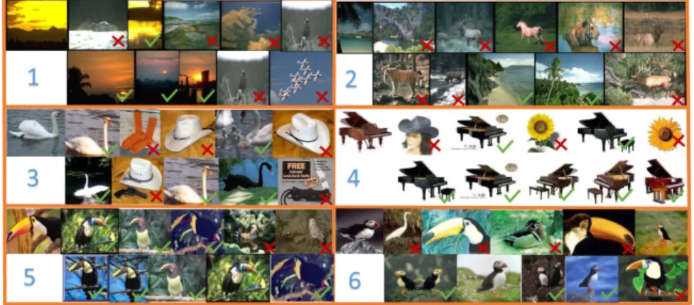
In the end, we randomly sample several query images and compare the top 5 ranked images retrieved with different metrics. Figure 7 shows the qualitative comparisons of
270
six different queries obtained by GMML and EMGMML. Generally, EMGMML re-trieves more relevant images compared with GMML. For instance, for query 4, EMG-MML obtained all of the 5 images, while GEMG-MML only obtained 2. This visual result clearly implies that EMGMML is much more effective than GMML in learning metrics for multiple modalities.
275
5. Conclusion and Future Work
We have introduced a general framework of multi-modal metric learning based on Geometric Mean Metric Learning to learn a metric for high-dimensional multi-modal data. Traditional metric learning approaches aim to learn a global linear metric, which is not applicable for handing multiple modalities. In this study, we have paid more
280
Figure 7: Examples of image retrieval on Corel 800, Caltech 10 and Birds from top to bottom by GMML (first row) and EMGMML (second row). ”√” represents the images of the same class with the queries, and ”×” represents the images from different classes.
modalities. The proposed method has the following advantages over most of exist-ing methods: 1) the learned metric achieves excellent performance compared with the state-of-the-arts; 2) its time complexity is only related to the maximum dimension of the modalities rather than the entire dimension nor the sample size. Extensive
exper-285
iments on image data for visual search demonstrate the excellent performance of our method.
In practical applications, only a small amount of data are labeled while the ma-jority remain unlabeled. Therefore, how to make full use of these massive unlabeled data arouse great attention. Moreover, as the kernel technique has been showed
it-290
s advantages in mining complex patterns, we are eager to exploit such technique for metric learning. In future work, we would like to apply geometric mean metric for semi-supervised and multiple kernel sceneries [37].
6. Acknowledgments
This work is partly supported by National Program on Key Basic Research Project
295
under Grant 2013CB329304, National Natural Science Foundation of China under Grants 61222210, 61432011, U1435212 and 61502332, and Q. Hu is supported by New Century Excellent Talents in University under Grant NCET-12-0399.
References
[1] K. Chang, K. W. Bowyer, S. Sarkar, B. Victor, Comparison and combination
300
of ear and face images in appearance-based biometrics, IEEE Transactions on Pattern Analysis and Machine Intelligence 25 (9) (2003) 1160–1165.
[2] S. Sarkar, Z. Liu, Evaluation of gait recognition, in: Encyclopedia of Biometrics, Springer, 2009, pp. 281–289.
[3] Q. Zheng, A. Kumar, G. Pan, Suspecting less and doing better: new insights on
305
palmprint identification for faster and more accurate matching, IEEE Transactions on Information Forensics and Security 11 (3) (2016) 633–641.
[4] A. Morales, A. Kumar, M. A. Ferrer, Interdigital palm region for biometric iden-tification, Computer Vision and Image Understanding 142 (2016) 125–133.
[5] J. Lu, X. Zhou, Y.-P. Tan, Y. Shang, J. Zhou, Neighborhood repulsed metric
learn-310
ing for kinship verification, IEEE Transactions on Pattern Analysis and Machine Intelligence 36 (2) (2014) 331–345.
[6] J. Lu, Y.-P. Tan, G. Wang, Discriminative multimanifold analysis for face recog-nition from a single training sample per person, IEEE Transactions on Pattern Analysis and Machine Intelligence 35 (1) (2013) 39–51.
315
[7] J. Lu, G. Wang, P. Moulin, Localized multifeature metric learning for image-set-based face recognition, IEEE Transactions on Circuits and Systems for Video Technology 26 (3) (2016) 529–540.
[8] B. Y. Li, M. Xue, A. Mian, W. Liu, A. Krishna, Robust rgb-d face recognition using kinect sensor, Neurocomputing 214 (2016) 93–108.
320
[9] I. A. Kakadiaris, G. Passalis, G. Toderici, M. N. Murtuza, T. Theoharis, 3d face recognition., in: BMVC, 2006, pp. 869–878.
[10] R. Wang, S. Shan, X. Chen, Q. Dai, W. Gao, Manifold-manifold distance and its application to face recognition with image sets, IEEE Transactions on Image Processing 21 (10) (2012) 4466–4479.
[11] J. Lu, V. E. Liong, X. Zhou, J. Zhou, Learning compact binary face descriptor for face recognition, IEEE Transactions on Pattern Analysis and Machine Intelli-gence 37 (10) (2015) 2041–2056.
[12] Y. Chen, J. Su, Sparse embedded dictionary learning on face recognition, Pattern Recognition 64 (2017) 51–59.
330
[13] C. Hu, X. Lu, M. Ye, W. Zeng, Singular value decomposition and local near neighbors for face recognition under varying illumination, Pattern Recognition 64 (2017) 60–83.
[14] F. Wang, B. Zhao, C. Zhang, Unsupervised large margin discriminative projec-tion, IEEE Transactions on Neural Networks 22 (2011) 1446–1456.
335
[15] S. C. Hoi, W. Liu, M. R. Lyu, W.-Y. Ma, Learning distance metrics with con-textual constraints for image retrieval, in: Proceedings of the Nineteenth IEEE Conference on Computer Vision and Pattern Recognition, 2006, pp. 2072–2078.
[16] S. C. Hoi, W. Liu, S.-F. Chang, Semi-supervised distance metric learning for col-laborative image retrieval, in: Proceedings of the Twenty First IEEE Conference
340
on Computer Vision and Pattern Recognition, 2008, pp. 1–7.
[17] G. Niu, B. Dai, M. Yamada, M. Sugiyama, Information-theoretic semi-supervised metric learning via entropy regularization, Neural Computation 26 (8) (2014) 1717–1762.
[18] S. T. Roweis, L. K. Saul, Nonlinear dimensionality reduction by locally linear
345
embedding, Science 290 (5500) (2000) 2323–2326.
[19] J. B. Tenenbaum, V. De Silva, J. C. Langford, A global geometric framework for nonlinear dimensionality reduction, Science 290 (5500) (2000) 2319–2323.
[20] Y. Mu, W. Ding, D. Tao, Local discriminative distance metrics ensemble learning, Pattern Recognition 46 (8) (2013) 2337–2349.
350
[21] A. Bellet, A. Habrard, M. Sebban, A survey on metric learning for feature vectors and structured data, arXiv preprint arXiv:1306.6709.
[22] J. Hu, J. Lu, J. Yuan, Y.-P. Tan, Large margin multi-metric learning for face and kinship verification in the wild, in: Asian Conference on Computer Vision, Springer, 2014, pp. 252–267.
355
[23] B. McFee, G. Lanckriet, Learning multi-modal similarity, Journal of Machine Learning Research 12 (2) (2011) 491–523.
[24] X. Lu, Y. Wang, X. Zhou, Z. Ling, A method for metric learning with multiple-kernel embedding, Neural Processing Letters 43 (3) (2016) 905–921.
[25] H. Xia, S. C. Hoi, R. Jin, P. Zhao, Online multiple kernel similarity learning for
360
visual search, IEEE Transactions on Pattern Analysis and Machine Intelligence 36 (3) (2014) 536–549.
[26] P. Wu, S. C. Hoi, P. Zhao, C. Miao, Z.-Y. Liu, Online multi-modal distance metric learning with application to image retrieval, IEEE Transactions on Knowledge and Data Engineering 28 (2) (2016) 454–467.
365
[27] P. H. Zadeh, R. Hosseini, S. Sra, Geometric mean metric mearning, in: Proceed-ings of the Thirty Third International Conference on Machine Learning, 2016.
[28] A. Papadopoulos, Metric spaces, convexity and nonpositive curvature, European Mathematical Society, 2005.
[29] S. Sra, R. Hosseini, Conic geometric optimization on the manifold of positive
370
definite matrices, SIAM Journal on Optimization 25 (1) (2015) 713–739.
[30] R. Bhatia, Positive definite matrices, Princeton university press, 2009.
[31] S. Lazebnik, C. Schmid, J. Ponce, A maximum entropy framework for part-based texture and object recognition, in: Proceedings of the Tenth IEEE International Conference on Computer Vision, Vol. 1, IEEE, 2005, pp. 832–838.
375
[32] E. P. Xing, A. Y. Ng, M. I. Jordan, S. Russell, Distance metric learning with application to clustering with side-information, Advances in Neural Information Processing Systems 15 (2003) 505–512.
[33] Y. Zhen, D.-Y. Yeung, A probabilistic model for multimodal hash function learn-ing, in: Proceedings of the Eighteenth ACM SIGKDD International Conference
380
on Knowledge Discovery and Data Mining, ACM, 2012, pp. 940–948.
[34] G. Chechik, V. Sharma, U. Shalit, S. Bengio, Large scale online learning of image similarity through ranking, Journal of Machine Learning Research 11 (3) (2010) 1109–1135.
[35] B. Xu, J. Bu, C. Chen, D. Cai, X. He, W. Liu, J. Luo, Efficient manifold ranking
385
for image retrieval, in: Proceedings of the Thirty Fourth International ACM SI-GIR Conference on Research and Development in Information Retrieval, ACM, 2011, pp. 525–534.
[36] Y. Ying, P. Li, Distance metric learning with eigenvalue optimization, Journal of Machine Learning Research 13 (1) (2012) 1–26.
390
[37] J. Liang, Y. Han, Q. Hu, Semi-supervised image clustering with multi-modal in-formation, Multimedia Systems 22 (2) (2016) 149–160.