Discussion Papers
Department of Economics
University of Copenhagen
Øster Farimagsgade 5, Building 26, DK-1353 Copenhagen K., Denmark
Tel.: +45 35 32 30 01 – Fax: +45 35 32 30 00
ISSN: 1601-2461 (online)
No. 09-13
An I(2) Cointegration Model With Piecewise Linear Trends:
Likelihood Analysis And Application
Takamitsu Kurita, Heino Bohn Nielsen,
and Anders Rahbek
AN I(2) COINTEGRATION MODEL
WITH PIECEWISE LINEAR TRENDS:
LIKELIHOOD ANALYSIS AND APPLICATION
Takamitsu Kurita
∗, Heino Bohn Nielsen
†and Anders Rahbek
‡July 6, 2009
Abstract: This paper presents likelihood analysis of the I(2) cointegrated vector autoregression with piecewise linear deterministic terms. Limiting behavior of the maximum likelihood estimators are derived, which is used to further derive the limit-ing distribution of the likelihood ratio statistic for the cointegration ranks, extendlimit-ing the result for I(2) models with a linear trend in Nielsen and Rahbek (2007) and for I(1) models with piecewise linear trends in Johansen, Mosconi, and Nielsen (2000). The provided asymptotic theory extends also the results in Johansen, Juselius, Fry-dman, and Goldberg (2009) where asymptotic inference is discussed in detail for one of the cointegration parameters. To illustrate, an empirical analysis of US consump-tion, income and wealth, 1965−2008, is performed, emphasizing the importance of a change in nominal price trends after1980.
Keywords: Cointegration, I(2), Piecewise linear trends, Likelihood analysis, US consumption.
JEL Classification: C32.
1
Introduction
This paper presents the complete asymptotic likelihood analysis of the I(2) cointegrated vector autoregression (VAR) with piecewise linear trends, i.e. a model where the slopes of the deterministic trends and the equilibrium means are allowed to change at known breakpoints. Our aim is to provide the asymptotic analysis with a focus on making infer-ence on the cointegration ranks and testing hypotheses on the cointegrating parameters based on likelihood ratio (LR) statistics. Thus we derive in Theorem 2 the asymptotic distributions of the maximum likelihood estimators (MLEs) of the parameters based on
The authors thank David F. Hendry, Søren Johansen and Bent Nielsen for helpful comments.
∗ Faculty of Economics, Fukuoka University, Bunkei Center Building, 8-19-1 Nanakuma, Johnanku,
Fukuoka, 814-0180, Japan. Supported by grant JSPS KAKENHI (19830111)
† Department of Economics, University of Copenhagen, Øster Farimagsgade 5, Building 26, DK-1353 Copenhagen K, Denmark.
a normalization suitable for deriving the limit distribution of the rank test statistic, see Corollary 2, and LR statistics on the cointegration parameters (∗, see below) also dis-cussed in Johansen et al.(2009). We thereby extend the analysis in Nielsen and Rahbek (2007), where cointegration rank testing is considered for I(2) models including a con-stant linear trend and level, and the analysis in Johansen et al. (2000), where the I(1) cointegration rank test is considered for models with piecewise linear trends. The paper complements the results in Johansen et al. (2009) by presenting limiting behavior of all estimators, also necessary for the results therein.
A main issue in the asymptotic analysis is the role of so-called impulse dummies as induced in the model by the inclusion of changing linear trends and levels, in addition to impulse dummies included in the econometric analysis to improve thefit. We demon-strate that the parameters loading the impulse dummies are inconsistent, but bounded in probability, which again implies that they play no role in the asymptotic distribution of the MLEs or the rank test statistic.
Empirically, the I(2) model with piecewise linear trends appears to be highly relevant. Many OECD countries have experienced pronounced shifts in inflation rates since the 1960’ties, leading to smooth changes in the trend slopes of nominal variables, and time series for nominal variables over the post-World War II period seems to be well described as autoregressive processes integrated of order two, I(2), seeinter alia Juselius (1998; 1999), Diamandis, Georgoutsos, and Kouretas (2000), Banerjee, Cockerell, and Russell (2001), Fliess and MacDonald (2001), Nielsen (2002), Bacchiocchi and Fanelli (2005), and Nielsen and Bowdler (2003) for applications of the cointegrated I(2) model. More abrupt changes in trend slopes are often related to new institutional regimes, and a simple modelling alternative in that case would be is to allow deterministic changes in trend growth for nominal variables. In the light of visible changes in mean growth rates, deterministic changes in trend slopes are undoubtedly a more relevant alternative to the hypothesis of double unit roots than a constant trend. More generally, it is known to be extremely important to have a relevant deterministic specification of the model before the presence of unit roots is tested, seeinter alia Perron (1989).
To illustrate the use of the I(2) VAR with piecewise linear trends, the methodology is applied to quarterly observations of nominal variables for US consumption, income and wealth, 1965−2008. We find a significant difference in the trend slope before and after
1981, a break that can be attrributed to a shift in policy focus following the stagflation period and the recession in 1981. Based on the LR test we find clear evidence of I(2) trends in the nominal variables, also when we allow for the deterministic change in the trend. In the model with a piecewise linear trend we accept homogeneity between nominal variables; this excludes money illusion in the long-run, and facilitates a nominal-to-real transformation from I(2) to I(1), Kongsted (2005), so that the equilibrium relationships may be formulated in real magnitudes for consumption, income, and wealth together with an interest rate and inflation. Homogeneity, and hence the validity of the theoretically relevant I(2)-to-I(1) transformation, is strongly rejected in a constant trend model.
The organization of this paper is as follows. Section 2 introduces the relevant repre-sentations of the VAR model for I(2) processes in the presence of changing linear trends. Section 3 then investigates the limiting behavior of the MLEs and the LR statistic for cointegration ranks. Finally, Section 4 presents the empirical illustration. Proofs are given in the appendix.
Throughout use is made of the following notation: for any × matrix of rank , , let ⊥ indicate a×(−) matrix whose columns form a basis of the orthogonal complement of span(). Set ¯ =(0)−1 such that0 =0 is the orthogonal projec-tion matrix onto span(). The symbols → and → are used to indicate weak convergence and convergence in probability respectively. Finally, we use[]to denote the largest inte-ger smaller than ∈R, and 1 () the indicator function which equals one if is true, zero otherwise.
2
The Model
2.1
The I(2) model with no deterministic terms
To introduce the notation consider initially the unrestricted VAR model with ≥2lags and parametrized conveniently for I(2) analysis of the-dimensional
∆2=Π−1−Γ∆−1+Ψ∆2X−1+ = 12 (1)
Here Π and Γ are (×)-dimensional matrices, Ψ∆2X−1 = P=1−2Ψ∆2−, with Ψ
(×) matrices and is a−dimensional i.i.d. (0Ω) sequence,Ω0. Furthermore,
the initial values 0∆0 and ∆2X0 are conditioned upon. The I(2) model, ( ), is
then defined by two reduced rank restrictions,
Π=0 and0⊥Γ⊥=0 (2)
with and (×) dimensional matrices, and are (−)× matrices with ≤ and≤−. The two reduced rank restrictions lead to the following reparametrization for likelihoodbased estimation,
∆2=[00−1+0∆−1] +⊥Ω00∆−1+Ψ∆2X−1+ (3)
whereis((+)×)dimensional, is(×(+)),is(×), andis((+)×(−)). Finally,⊥Ω=Ω⊥(0⊥Ω⊥)−1 is(×(−))dimensional.
To interpret the parameters and the dynamics ofwe need the following assumption:
Assumption 1 Assume that the characteristic polynomial, () = (1−)2 −Π+
Γ(1−)−P=1−2Ψ(1−)2, has exactly2(−)−roots at= 1and the remaining
Under Assumption 1, ∆2
, = 00+0∆ and 0∆ all have a stationary
representation and hence is a (multi-)cointegrated I(2) process, see also Johansen
(1997).
The original parameters in (1), imposing the reduced rank restrictions in (2), can be derived from the parameters in (3) as follows: First write write ⊥ = (⊥1 ⊥2) and
⊥= (⊥1 ⊥2)where⊥1 =⊥,⊥1 =⊥ ⊥2 = ( ⊥1)⊥,⊥2 = ( ⊥1)⊥. Then it holds that = ( ⊥1), = , 0 = −Ω−1Γ, with Ω−1 =Ω−1
¡
0Ω−1¢−1, and 0 =−0⊥Γ( ⊥1) =−(0⊥Γ ), using the skew-projection identity,
0Ω−1+⊥Ω0⊥ = (4)
Furthermore, the parameters ,,,,Ψ and Ω are all freely varying and estimates are obtained by a switching algorithm: For fixed , the parameters ⊥ and can be obtained by solving an eigenvalue problem and the remaining parameters can be found from ordinary linear regression. For fixed values of these parameters, can be estimated by generalized least squares, see Johansen (1997) for more details.
2.2
Deterministic terms
Our focus will be on the inclusion of piecewise linear trends in the I(2) model. Specically, we allow for a linear deterministic trend and changes in the trend slopes and equilibrium levels. The deterministic terms enter the model to allow piecewise linear trends in all directions of the process, including the multi-cointegrating relationships, and are restricted to avoid quadratic and higher order trends.
Let therefore= (0 1 )0 denote a generic(+ 1)-dimensional
determinis-tic linearly trending variable, and set=∆. Make the following assumption:
Assumption 2 For the deterministic(+ 1)−dimensional linear trend= (0 )0
assume that with ∈ [01], −1
[ ] → on the space of (+ 1)-dimensional cadlag
functions on [0,1], where
−1[ ]→ as → ∞ = 01
Furthermore, it is assumed that, as → ∞,
−3 X =1 0 → Z 1 0 0
which is a positive difinite (+ 1)×(+ 1)matrix.
Set 0 = and hence 0 = that is, the first component of is throughout
a linear trend, while for = 1 allow linearly independent changing linear
trends. A changing trend slope at say = 1 with 1 1 can be represented
by defining 1 = (−(1−1)) 1 (≥1), such that 1 = (−1) 1 (≥1), with
the discrete time interval [1 ], 1 denotes the corresponding (limiting) fraction in the
continuous time interval[01]. Likewise for general,= 12 .
With=∆we have[ ]→ 6= 0by Assumption 2. In terms of1just defined,
we have for example1=∆1= 1 (≥1) and hence1= 1 (≥1).
2.2.1 Constant linear trend
The case of = 0 = , which allows for a linear trend in all linear combinations of
the I(2) process , is analyzed in Rahbek, Kongsted, and Jørgensen (1999) and Nielsen
and Rahbek (2007) and it is briefly reviewed here before introducing the changing linear trends, see also Paruolo (2000) for other specifications.
Let=,= 1and define∗ = (0 )0Then the I(2) model with a linear trend
is conveniently given by,
∆2=[0∗0∗−1+∗0∆∗−1] +⊥Ω0∗0∆∗−1+Ψ∆2X−1+ (5)
where∗= (0 0)0((+ 1)×(+)), while∗=¡0 0¢0 ((+ 1)×)and the remaining parameters are as in (3).
Under Assumption 1, it was shown in Rahbek et al. (1999: Theorem 2.1) that indeed in (5) is an I(2) process with the representation,
=2 P =1 P =1 +1 P =1 +++0() (6) 2 =⊥2(0⊥2Θ⊥2)−10⊥2 01 = ¯0Γ2 0⊥11 = ¯0⊥1(−Θ2)
Here 0() = P∞=10− is a stationary mean-zero I(0) process with exponentially
decaying coefficients1 and Θ=Γ0Γ+−P=1−2Ψ. The coefficients and for the
trend and level, respectively, depend on and as well as on the initial values of the
process.
It follows from (6) that ∗0∗ = 0+0 is I(1) whereas the (−−) linear
combinations 0⊥2 are I(2). In other words, ∗0∆∗ and 0⊥2∆2 are mean zero
sta-tionary, or I(0), processes in addition to the mean-zero stationary linear combinations given by,
∗ =0∗0+∗0∆∗
2.2.2 Changing linear trend
One may view the resulting model in (5) as derived from the I(2) model with no de-terministic terms in (3), replacing by (0 )0 = (0 1)0, and likewise for ∆
and ∆2−. This would however lead to an overparametrized model, and instead by
the analysis in Rahbeket al.(1999), this results in the model in (5) with replaced by
∗ = (0 )0, and ∆replaced by∆∗= (∆0 )0. Note that∆2=∆= 0and
∆2∗− =∆2− enters unchanged.
1
Consider next extending to include the additional changing linear trends from
Section 2.2. Initially, observe that in this case, with a changing linear trend such as 1 = (−(1−1)) 1 (≥1), then ∆21= 1 (=1) =1, say, where1 6= 0. That
is, the second order difference of the changing trend is an impulse dummy. Likewise with ∆21=∆16= 0, where1=∆1. Note that including(1∆1)0 as an unrestricted
regressor is equivalent to include(1 1−1)0, and below we include impulse dummies and
not their differences. Introduce for that purpose , which is an -dimensional variable
of impulse dummies,
= (1 )0 where= 1 (=) for some,1 , = 12 .
Then, similar to the constant trend case, we extend the I(2) model to allow for chang-ing linear trends by includchang-ing ∗ = (0 0)0, ∆∗ = (∆0 0)0 but now also impulse dummies inin the model, denoted ( ) :
∆2=[0∗0∗−1+∗0∆∗−1] +⊥Ω0∗0∆∗−1+Ψ∆2X−1+Ψ+ (7)
where∗= (0 0)0 is((++ 1)×(+)), and∗=¡0 0¢0 is((++ 1)×). The remaining parameters are as in (3), except the additional Ψ (×) parameter. Note
that the inclusion of the impulse dummies in as unrestricted regressors implies that
ˆ = 0, whereˆ are the estimated residuals in (7).
In empirical models, theimpulse dummies inare included for two different reasons.
First of all,includes the impulse dummies resulting from the changing linear trends
(and levels). Specifically, with the example of 1, this leads to the inclusion of 1−,
= 0 −1 which are impulse dummies for = 1 +. With changing linear
trends, a total of impulse dummies should thus be included in . As noted above,
thecorresponding estimated residualsˆ1 ˆ1+(−1) all equal zero, and the inclusion
of these dummies is therefore equivalent to conditioning on1+(−1)∆1+(−1)and ∆X2
1+(−1) in estimation. In addition to these induced impulse dummies, we allow
for further impulse dummies , and hence ≥ . The additional impulse dummies
entered as unrestricted regressors are sometimes referred to as innovation dummies and are common in empirical I(2) analyses since they often lead to a better empirical fit of the model within sample. We demonstrate below that they play no role in the asymptotic analysis, and the precise specification of is not important asymptotically. Likewise for
so-called transitory impulse dummies, defined as∆= 1(=1)−1(=1+ 1).
It follows directly by Rahbeket al. (1999) that the representation of is identical to
(6), with the only exception that nowis replaced by =+Ψ. We thus immediately
get that under Assumption 1, in (7) has the representation,
=2 P =1 P =1 +1 P =1 +++0() (8)
This was also used in Johansen et al. (2009: proof of Lemma 1) where a generic infinite sum of impulse dummies is introduced to faciliate the interpretation. Define here such a
generic infinite sum,
=() (9)
with () = P∞=0, exponentially decreasing, and impulse dummies. The
idea is that vanishes asymptotically as noted above and in this sense unimportant
for the representation of . For example, 0() contains such a vanishing term,
0()Ψ(=).
Thus, from (8) it holds that is an I(2) process with broken linear trends and
levels, and that ∆2−
¡
∆2
¢
is I(0) with¡∆2
¢
= , a generic infinite sum of
impulse dummies. Likewise, ∗0∆∗ = 0∆+0 is I(0) except for (∗0∆∗) =
. Finally, the linear combinations given by 0∗0 +∗0∆∗ are I(0) except for
¡0∗0+∗0∆∗
¢
= . Thus in this sense the interpretation remains identical to
the linear trend case, except for the additional asymptotically vanishing infinite sums of impulse dummies, again generically referred to as. In the empirical application below,
we illustrate the role of the impulse dummies and the interpretation of the deterministic terms.
3
Likelihood Inference
3.1
Estimation
Under ( ), ML estimators in (7) are obtained by the usual switching algorithm described above for the I(2) model with no deterministic terms. Note that the loading the impulse dummies,Ψ, is estimated from single observations only, and hence are bounded
but inconsistent, see Theorem 1.
3.2
The rank test statistic
For determination of the cointegration ranks, and , we consider the LR statistic for ( ) against the unrestricted alternative() =(0), and it is defined by,
()=−log ¯ ¯ ¯ΩˇΩˆ−1 ¯ ¯ ¯
where Ωˇ and Ωˆ denote the covariance matrices estimated under ( ) and (),
respectively.
3.3
Asymptotics
When reporting results for the asymptotics of the parameter estimators emphasis will be on the parameters∗= (0 0)0,∗=¡0 0¢0andThe parameters ΨandΩhave the same asympotic behaviour as in the model with no deterministic terms analysed in Johansen (1997). As shown the remaining parameterΨ plays no role for the asymptotic
analysis, and we also note in this respect thatΨˆ is not consistent. We start by providing
their asymptotic distributions are used to derive the limiting behaviour of the LR statistics for rank and linear hypotheses respectively.
3.3.1 Theoretical parameters
In the followingˆ denotes the ML estimator of a parameter , while 0 denotes the true
value. Furthermore, the parameters , and ⊥ under ( ) are normalized on ¯0,
¯
0 and¯0⊥Ω respectively such that ¯00=,¯00 =+, and¯⊥0 Ω0⊥ =−. These are
theoretically convenient normalisations which ensure identification of all parameters in the model. Note in particular that= ¯0
0 which is(+)×. Define next the parameters,
00 = (−0)0¯⊥20 01 = (−0)0¯⊥10 0 = 0(−0)0 20 = (−0)0¯⊥20=0(−0)0¯⊥20 00 = 0⊥( −0)0¯⊥20 0 = (−0)0−(−0)0¯000 0 = ⊥0 (−0)0 (10)
Note that 0 1 2 and are identical to the definitions in Johansen (1997), while
and are new parameters corresponding to the deterministic terms.
We first turn to consistency of the just defined parameters, with the proof given in appendix:
Theorem 1 For the model ( ) under Assumption 1 the ML estimators exist with probability tending to one, and using the definitions in (10),
³
12ˆ00 12ˆ10 32ˆ20 ˆ0 ˆ0´0 → 0 and ³12ˆ00ˆ0 ´0→ 0 (11)
as → ∞. Moreover, 12(ˆ−0) → 0, and ˆ ˆ Ψˆ and Ωˆ are consistent. Finally, ˆ
Ψ = (1).
Theorem 1 establishes also rates of convergence and the next theorem gives the as-ymptotic distributions these estimators. To report these some definitions are neededfirst. Define first for and of dimension and defined on the unit interval
∈[01], | = −R010 ³R1 00 ´−1 ( ) = R010³R1 00 ´−1R1 0 0 ( ) = ³R010 ´−1R1 0 0 (12)
And next define the process by,
=
¡
00 10 20¢0 =¡020⊥2 010⊥1R0020⊥2¢0 (13) with a Brownian motion on ∈[01]with covariance Ω0. Furthermore, define
1 = ¡ 00Ω−010 ¢−1 00Ω−01 (14) 2 = ¡ 00Ω−010¢−100Ω−01 (15) where00= ¯0⊥000⊥Ω0.
Theorem 2 For the model( ) under Assumption 1, ³ ˆ00 ˆ10 2ˆ20 32ˆ0 12ˆ0´0 → ∞ = ¡0∞0 1∞0 2∞0 ∞0 ∞ 0¢0 =(∗ 1) ³ ˆ00 12ˆ0 ´0→ ∞ = (0∞0 ∞0)0=(0∗ 2) as → ∞. Here ∗
= (0 0 0)0 and 0∗ = (00 0)0 with defined in (13) and
1 2 are defined in (14)-(15). Moreover, and are defined in Section 2.2.
Finally, (ˆ−0) → ¯00⊥101∞ while the remaining parameters are asymptotically Gaussian. In particular,12 ³ ˆ 0−0 0 ´ →×(2++) ¡ 0Ω0⊗Σ−001 ¢ , where0 defined in (27) in the appendix is the coefficient for the (asymptotically) stationary relations 0
in (26) of the model, and Σ00=Var(0).
3.3.2 Asymptotics for hypotheses on individual parameters
From Theorem 2 limiting distributions for ˆ∗ and ˆ∗, normalized on known constants rather than as here the true parameters, are straightforward to derive using the definitions in (10) analogous to Johansen (1997: Theorems 3, 4 and 5). Likewise for other parameters in the model by exploiting their definitions in terms of the parameters and in
Theorem 2. To examplify we derive the limiting distribution of ˆ∗ =¡ˆ0ˆ0¢0 when is normalized by a known constant×(+) dimensional matrix say, that is
ˆ ∗= ˆ∗¡0ˆ¢−1 = à ˆ ˆ ! . (16)
Withsuch that00 =+ we have the following corollary:
Corollary 1 For ˆ∗ defined in (16) it follows that,
à ¯0⊥20(ˆ−0) √ (ˆ−0) ! →∞¯0⊥0
which is mixed Gaussian.
The proof is given in the appendix. An immediate implication of the result is that likelihood ratio tests for linear hypotheses as applied in Section 4 of the form ∗ = , with a known ((++ 1)×)-dimensional matrix, + ≤ ≤ + + 1 and
(×(+))-dimensional, are asymptotically 2 distributed. A thorough discussion of hypothesis testing on the I(2) cointegration parameters as well as is given in Johansen (2006) and Boswijk (2000) for the I(2) model with no deterministics, which in Johansen
et al.(2009) are applied for a general discussion on 2-based inference on ∗ =∗and ∗ in the extended model here. Note in this respect, that Johansenet al. (2009) consider in particular the distribution of ∗ under general and empirically relevant identifying restrictions. These results may also be derived from our Theorems 1 and 2.
3.3.3 Rank Test Asymptotics
From the results in Theorem 2, and using Nielsen and Rahbek (2007), we get the as-ymptotic distribution of the rank test statistic as a corollary, with proof given in the appendix:
Corollary 2 Under Assumption 1, then as → ∞,
()→ ∞+∞() (17)
where∞ ={( )}and∞()=©¡2 () 2 ¢ª
. Here = (10 20)0 is a(−)dimensional standard Brownian motion, where1 is s-dimensional and 2 is
(−−)dimensional. Furthermore, = ¡¡10R020 0¢¯¯()¢ and () =
(20 0)0 with ∈[01].
The asymptotic distribution in (17) depends on and the timing of the changing trend slopes, (1 2 ), and for empirical applications the distributions have to be
simulated. Below we simulate this for a particular empirical example.
4
Empirical Illustration
To illustrate the theoretical results we conduct an empirical analysis of US quarterly consumption data,1964−2008. We consider the = 5dimensional vector:
= ( )0 (18)
where is nominal private consumption, is nominal disposable income after tax,
is nominal wealth including financial wealth and housing equity, while represents the
price level measured as the consumption deflator. These variables are all transformed by natural logs. To capture interest rate effects on savings, we include the annual bond yield, , divided by 4 to be comparable to a quarterly inflation rate, ∆. See Appendix B
for details of the data. Similar data sets for real rather than nominal variables have been analyzed in inter alia Lettau and Ludvigson (2001) and Palumbo, Rudd, and Whelan (2006).
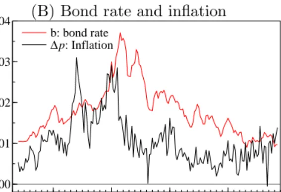
The time series are presented in Figure 1. In graph (A), the developments of the nominal variables,,and, are quite parallel, although the wealth variable,,fluctuates more. Recent discussions have referred to this as signs of ’bubbles’ in asset and house prices. The price index, , has increased less over time, but seems to share a similar smooth stochastic trend. We note that the trend slope seems to change just after 1980, both in the price deflator and in the nominal measures, and in the empirical analysis we allow for a deterministic change in the trend slope in 1981 : 2. The shift in trend slope reflects a change in policy focus following the stagflation period in late 1970’ties. The US entered a severe recession in July1981partly initiated by a contractionary monetary policy to dampen inflation, cf. the inflation rate (∆) and bond yield () in graph (B).
(A) Nominal variables, logs (B) Bond rate and inflation 1970 1980 1990 2000 13 14 15 16 c: consumption y: income (−0.2) w: wealth (−1.8) p: prices (+15) 1970 1980 1990 2000 0.00 0.01 0.02 0.03 0.04 b: bond rate Δp: Inflation
Figure 1: US data for the empirical analysis, 1964-2008. The time series in graph (A) have been shifted to have comparable means.
After the recovery of the US economy through 1982, the inflation rate stayed at more moderate values than the previous decade. Also note that inflation is clearly persistent, emphasizing the presence of I(2) trends in the data.
Statistical Analysis. The empirical analysis is based on a VAR with = 3 lags and the effective sample contains the = 175 observations from 1965 : 1 to2008 : 3, hence conditioning on observations for1964 : 2,1964 : 3, and1964 : 4. The model incorporates in addition to the standard constant and linear trend term, a change in levels and trend slopes in 1981 : 2 and hence three impulse dummies as well. The likelihood function of the unrestricted model seems to accounts for the main features of the data, and the hypotheses of no autocorrelation of order one and two are not rejected with 2(25) and 2(50) statistics of(1) = 36 and (2) = 63, respectively. There are several outlying residuals in the model, however, associated with special events and large shocks in the sample period, and the Jarque Bera test for the null hypothesis of Gaussian residuals is rejected with a2(10) statistic of
= 178. We will refer to this as thebaseline model
in the following.
To account for a number of the large shocks in the sample period, and to restore normality of the residuals, we also consider a version of the model that includes nine additional impulse dummies in , defined to take the value one in 1972 : 4, 1974 : 1,
1975 : 2, 1980 : 2, 1982 : 4, 1984 : 2, 1993 : 1, 1999 : 4, and 2008 : 2, respectively. For this, theaugmented model, the above hypotheses for no-autocorrelation and Gaussianity are not rejected ((1) = 34 (2) = 58, and = 17). Recall that the additional unrestricted impulse dummies do not change the asymptotic distributions of estimators and test statistics, and as we illustrate below, they only marginally change the finite sample results; in fact, all main conclusions of the empirical analysis are unchanged.
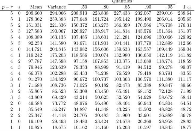
Quantiles − Mean Variance 50 80 85 90 95 Γ95 5 0 209660 294066 208913 223838 227433 232067 239016 23864 5 1 178362 259383 177648 191724 195142 199490 206014 20565 5 2 151031 221336 150372 163273 166399 170566 176708 17631 5 3 127583 190067 126927 138917 141814 145576 151364 15107 5 4 108089 163135 107485 118601 121281 124696 130066 12992 5 5 92253 141580 91671 101901 104441 107779 112899 11266 4 0 144721 204845 143982 156606 159633 163557 169449 16904 4 1 119242 175203 118586 130074 132980 136650 142119 14182 4 2 97787 147598 97158 107853 110375 113689 118774 11859 4 3 79946 123639 79353 88999 91419 94512 99278 9907 4 4 66078 102288 65433 74238 76529 79418 83791 8355 3 0 91270 134829 90672 100737 103303 106570 111380 11117 3 1 71688 108736 71025 80182 82473 85388 89847 8966 3 2 55865 86523 55309 63450 65491 68152 72128 7199 3 3 43869 69429 43214 50625 52520 54928 58672 5841 2 0 49588 73772 48976 56496 58404 60943 64804 6451 2 1 35549 56247 34897 41548 43225 45502 48828 4872 2 2 25347 41418 24705 30483 31960 33901 36889 3678 1 0 19109 29493 18480 23424 24678 26369 28958 2883 1 1 10825 18675 10162 14160 15203 16597 18843 1877
Table 1: Asymptotic distribution simulated from Corollary 2 with = 1and1= 0377.
Based on random walks with 2000 steps and 50.000 replications. Γ95 is the 95% quantile
of the approximatingΓ distribution.
Cointegration Ranks. To make inference on the cointegration ranks wefirst simulate the asymptotic distribution in (17) for the current = 1 and 1 = 0377. This is done
by replacing the Brownian motion with a random walk with 2000 steps, replacing
with a discrete time trend function, and replacing =∆ with the corresponding
discrete step function. The simulation here is based on50000replications and moments and quantiles are reported in Table 1. To calculate tail probabilities for the test statistics below the asymptotic distribution is also approximated by a Γ−distribution with the simulated mean and variance, see Doornik (1998), which closely reproduces the simulated quantiles, see Table 1.
Table 2 reports the LR statistics for the cointegration ranks for the baseline model, together with the asymptotic tail probabilities derived from the Γ−approximation. The hypotheses ( ) are tested sequentially against() based on the partial nesting
structure. All models with = 0 and = 1 are safely rejected. In the row for = 2 the reductions to the models(21)and(22)have tail probabilities around10%, and we note that in the augmented model with9additional impulse dummies the tail probabilities for the LR statistics for the two candiate models are 8% and 14%, respectively. The two potentially preferred models are nested,(21)⊂(22), and can be compared
−2 log¡( )¯¯()¢ 0 4428 [00] 3424 [00] 2608 [00] 2024 [00] 1677 [00] 1546 [00] 1 2485 [00] 1801 [00] 1293 [01] 1040 [02] 943 [01] 2 1248 [00] 854 [10] 672 [11] 588 [05] 3 543 [28] 425 [18] 315 [17] 4 221 [27] 124 [32] −− 5 4 3 2 1 0
Table 2: Likelihood ratio tests for the cointegration ranks,( ). The numbers in brackets are tail probabilities derived from the Γ−approximation of the simulated distribution in
Table 1.
directly using a LR test. It follows directly from the result in Corollary 2 that the likelihood ratio statistic for(21)|(22), calculated from the estimated covariances as
(21)|(22) =−log ¯ ¯ ¯Ωˆ(21)Ωˆ−(212) ¯ ¯ ¯
has the limiting distribution of the maximum eigenvalue of¡2 () 2 ¢
, see Nielsen (2007), which is easily simulated. For the baseline model the statistic is182, corresponding to a tail probability of 7%, while the augmented model produces a test of 205 and a tail probability of 3%, showing that the reduction to the model (21) is marginal.
Furthermore, the model(22)with −−= 1 I(2) trend is most easily reconsiled with economic theory and together with the statistical evidence we take this model as the preferred in the following, noting, however, that it could be interesting also to consider the economic implications of second I(2) trend in the data.
Note that there are strong indications of an I(2) trend in the data, even after allow-ing for a deterministic shift in the trend. For the baseline model with the hypothesis (22) imposed, the characteristic polynomial has four unit roots and the inverses of the remaining11 roots are given by,
067±021·; −042±005·; −011±038·; 028±026·; 033±008·; −022 which all have absolute values smaller than one, and hence there are no indications of additional unit roots.
Testing Homogeneity. Based on the preferred model (22), we first investigate if the change in the linear trend implied by 1 is needed, or equivalently, we test the
restriction of a common deterministic trend coefficient in all cointegrating relationships, 0, in the two sub-samples. We formulate this as,
H0 :∗ = Ã 6 0(1×6) !
withunrestricted, imposing a zero row in∗. The LR statistic forH0|(22)is given
by178corresponding to a zero tail probability in the asymptotic2(4)distribution. This emphasizes the relevance of the changing trend. In the augmented model with9additional impulse dummies the corresponding statistic is296confirming this.
An important hypothesis is that the common I(2) trend loads into the nominal vari-ables with equal coefficients, so that the real variables,−,−, and−, arefirst
order non-stationary, I(1). Economically, this hypothesis implies that money illusion is excluded in the long-run, and the hypothesis would allow a nominal-to-real transformation from the I(2) vector to a vector of I(1) variables, e.g.
= (− − −∆ )0
see Kongsted (2005). Given homogeneity, the subsequent I(1) cointegration analysis of
can be conducted without loss of information and the polynomially cointegrating relation-ships are embedded as usual cointegrating relationrelation-ships in the I(1) cointegration model, see Kongsted and Nielsen (2004). Often this hypothesis is imposeda priori, see e.g. the analyses of real consumption variables in Lettau and Ludvigson (2001) and Palumboet al.
(2006), but here we want to explicitly test the hypothesis of homogeneity.
Equal loadings to the single stochastic I(2) trend corresponds to⊥2being proportional to= (11110)0, see (8). From the baseline case and from the augmented model , the estimated counterparts are given by
ˆ
baseline⊥2 = (1 0918 1436 1163 0018)0 ˆ
augmented⊥2 = (1 0914 1263 1130 0029)0
respectively. The results suggest that the unrestricted estimates under(22)are quite close to homogeneous, except slightly larger coefficients toand. Noting that⊥2=⊥, the homogeneity restriction can be formally tested as
H1 :∗= Ã ⊥ 0(5×2) 0(2×4) 2 !
where⊥is a5×4matrix andis7×6with unrestricted parameters. The LR statistics forH1 are53and 34 in the two specifications, corresponding to tail probabilities of026
and049 in the asymptotic2(4)distribution.
For comparison, the homogeneity restriction in H1 has also been tested in the model
with no change in the linear trend (which is therefore misspecified). Without allowing for the changing trend slopes, the LR statistic is204and this would lead to afirm rejection of homogeneity of the stochastic trends, and, hence, a rejection of the economically relevant nominal-to-real transformation. Thus, the baseline model is well-specified and leads to sound economic interpretations of the dynamics, while the misspecified model where a change in the trend is not allowed for, leads to the reverse.
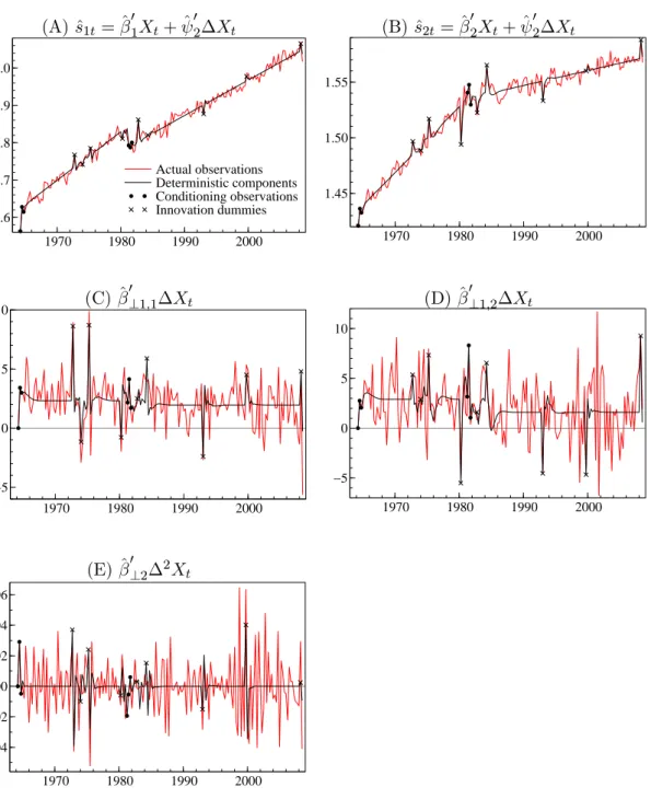
Deterministic Terms. To illustrate the role of the deterministic components, i.e. the effects of the trend with a changing slope in1981 : 2, the= 3impulse dummies induced by the changing trend slope, and the nine additional innovation dummies included to ac-count for outliers, Figure 2 shows the stable combinations,ˆ= ˆ0+ ˆ0∆,ˆ0⊥1∆,
and ˆ0⊥2∆2, together with their deterministic components. The deterministic
compo-nents of the data are calculated as the terms in (8) involving the deterministic variables, ,,, and the initial values,0,∆0, and ∆20:
2 P =1 P =1 Ψ+1 P =1 Ψ+++0()Ψ (19)
where and contain also the effects of the initial values of the process. We recall that the innovation dummies () enter the dynamics in the same way as the innovations
(), and accumulate (once and twice) to produce level shifts and changing trend slopes
in the data.
Graph (A) and (B) show the = 2 multi-cointegrating relationships, ˆ = ˆ0+
ˆ
0∆. Here we have normalized so that ˆ1 has unit coefficient to and excludes the
interest rate, , while ˆ2 is normalized on and excludes consumption, . Regarding
the deterministic components, wefirst note the marked linear trends in equilibrium. The break in 1981 : 2 allows for a shift in the equilibrium level and in the slope of the linear trend. For the chosen normalization, the consumption relation, ˆ1, has approximately
a constant trend slope, suggesting co-breaking between the trend breaks of individual variables. The changing trend slope is clearly important for the interest rate relation,
ˆ
2, however. Regarding the impulse dummies, we note that the induced dummies play
the role of conditioning on observations for 1981 : 2, 1981 : 3, and 1981 : 4, and the effect is comparable to the initial values, 1964 : 2, 1964 : 3, and 1964 : 4. In addition, Figure 2 highlights the observations modelled by innovation impulse dummies. From the accumulation in (19), with 02 = 0 and 01 6= 0, the impulse dummies give at most
level shifts inˆ0, but the accumulated effects cancel in the multi-cointegrating relations
producing only exponential decreasing effects,.
The I(1) directions of the data,ˆ0⊥1, also contain trends with a changing slope (and
a level shift) in 1981 : 2, and the first differences, ˆ0⊥1∆, are reported graph (C) and
(D). We note that the changing trend inˆ0⊥1 gives a change in the growth rates in the
graphs in1981 : 2. From (19), with 0⊥12 = 0 and 0⊥11 6= 0, the innovation dummies
produce level shifts in ˆ0⊥1, but they are eliminated in the graph by first differencing.
Note that thefirst differencing produce a slightly more complex behavior of, which, by
the way, is the same as the dynamic effect of hte normal innovations,.
Finally, the I(2) direction,ˆ0⊥2, contains a linear trend and the changing trend slope
in 1981 : 2. Furthermore, since 0⊥22 6= 0, the innovation dummies produce changing
slopes at nine additional points in time. Graph (E) shows the stationary transformation,
ˆ
0⊥2∆2. This has mean zero (from the double difference of the linear trends) apart from
(A)ˆ1= ˆ 0 1+ ˆ 0 2∆ (B) ˆ2= ˆ 0 2+ ˆ 0 2∆ 1970 1980 1990 2000 3.6 3.7 3.8 3.9 4.0 Actual observations Deterministic components Conditioning observations Innovation dummies 1970 1980 1990 2000 1.45 1.50 1.55 (C)ˆ0⊥11∆ (D) ˆ0⊥12∆ 1970 1980 1990 2000 −5 0 5 10 1970 1980 1990 2000 −5 0 5 10 (E)ˆ0⊥2∆2 1970 1980 1990 2000 −0.04 −0.02 0.00 0.02 0.04 0.06
Figure 2: Stationary linear combinations of the data based on the estimated augmented model, i.e. ˆ = ˆ0+ ˆ0∆, ˆ0⊥1∆, and ˆ0⊥2∆2, and their deterministic
com-ponents. The deterministic parts are the terms in (8) depending on , , , and the
For empirical applications a choice must be made between allowing an innovation dummy, producing changing trend slopes in the data that co-break by assumption, or allowing also changing trend in the equilibrium relationships. Economically, this amounts to choosing between large shocks that follow the usual dynamics of the normal innovations versus genuine regime shifts. In the application above this choice was based ona priori
reasoning and the graphical appearance of the data.
Software Implementation. The empirical analysis above was carried out in Ox, see Doornik (2002). Ox code for the I(2) rank test and for simulating the asymptotic dis-tribution in the case of changing trend slopes can be obtained from the authors. The cointegrated I(2) model and the likelihood ratio test for the cointegration ranks are also implemented in the software CATS in RATS, see Dennis (2006).
A
Asymptotics
A.1
Proof of Theorem 1
The I(2) model in (7) is a regression model with nonlinear parameters. To analyze this, it is as in Johansen (1997: Theorem A1) useful to initially analyze a linear regression model with regressors as in (7). With -dimensional, write the linear regression model as,
=00+11+22++++() (20)
where for = 12 , () is (0Ω) distributed, conditional on the regressors,
and pastand. The-dimensional regressorsare — apart from an asymptotically
vanishing termdefined in (9) in terms of impulse dummies— mean-zero I() processes
for= 012. Specifically, with the -dimensional independent of and i.i.d.(0Σ)
distributed
=+ where ∆ = () =
P∞
=0− and the coefficients
exponentially decreasing. Furthermore, = which is-dimensional and which
satisfies Assumption 2 and = with = ∆. Finally is a -dimensional
impulse dummy regressor with entries = 1 (=),1 , and = [ ] with
∈]01[.
Lemma 1 Set = ¡0 1 2 ¢ and = ¡ ¢∈ Θ ⊂ R, where Θ is closed andΩ0 varies freely. Then for the MLE ˆ it holds that
−1³ˆ−0´→ 0 (21)
as → ∞and with =blockdiag(0 −121 −322 −1 )Furthermore,
³ ˆ −0 ´ =(1). Proof: Define = ¡ 0 0 10 20 0 0 ¢0, = (00 10 20 0 0 )and set =
(0). Moreover, use the notation that for any and dimensional time seriesand
respectively, = 1 P =1 0 (22)
Next, note that
³ ˆ −0´ = ·−1 · = ¡−−1 ¢ ¡ −−1 ¢−1
By definition of the-dimensional impulse dummy , and the generic defined in (9),
standard limit arguments immediately give, · = +(1). That
is, the OLS correction for is asymptotically negliable, and moreover, = +
behaves asymptotically as for= 01 and2. Hence,
· = + (1) → Ã Σ00 0 0 R010 ! (23)
where Σ00 = (0) = P∞=00Σ000 and = (10 20 0 0)0. Here 1 =
1(1) and 2 = 2(1)
R
0
with a Brownian motion with variance Σ0.
Similarly, 12·=12+(1) → µ 0×(0Σ00⊗Ω0) Z 1 0 0 ¶ (24) where is a -dimensional Brownian motion with variance Ω0. Collecting terms (21)
holds. Note that it is essential for the results that the asymptotically stationary 0 =
0+regressor has mean zero apart from the generic defined in (9) which is
asymp-totically vanishing. If not, e.g. the blockdiagonality in (23), which corresponds to the limiting information, would not apply.
Finally, with each entry in the -dimensional of the form = 1 (=), it
follows thatˆ=(ˆ)−1= ³ −ˆ ´ −1, or ³ ˆ −0´=³1− ³ ˆ −0´1 − ³ ˆ −0´ ´ =³1 ´ +(1)
from whichˆ = (1)and inconsistency holds. ¤
Proof of Theorem 1: Rewrite the I(2) model( ) in (7) as in (20),
∆2=00+11+22++++() (25) where =−1, =−1,2=0⊥20−1,=Ψand 0= ⎛ ⎜ ⎝ 00−1+00∆−1+0000−1+00−1 00∆−1+00−1 ∆2X−1 ⎞ ⎟ ⎠ 1= Ã 0⊥20∆−1 0⊥10−1+0⊥10¯000−1 ! (26)
Recall that = ¯00, such that = 0+ ¯00⊥101 = (1), implying ⊥ = ⊥(1) as
well. Using the definitions in (10), the parameters0 1 and2 are given by (27), 0 = ¡ (−0)0¯0+⊥Ω0Ψ
¢
1 = (00 +⊥Ω0[¯⊥(1)00 + ¯(1)20] 10)
2 = 02
(27)
while the parameters for the deterministic regressors are given by,=Ψ,
=0 and = (0+⊥Ω0[¯⊥(1)0 + ¯(1)0 ]) (28)
Applying our Lemma 1, the proof is identical to the proof of Theorem 2 in Johansen (1997), apart from the and parameters in (28), and hence and in (10).
As ˆ = ˆˆ0 , with ˆ consistent, we can conclude by Lemma 1 that ˆ → 0. Next,
with defined in (28), multiply by ˆ⊥ to see that ˆ
→ 0, as ˆ⊥ˆ ˆ Ωˆ ˆ⊥ and ˆ1
andˆ are consistent. Likewise, multiplying byˆ0Ωˆ−1givesˆ
A.2
Proof of Theorem 2
The proof proceeds basically as in the proof of Lemma 1 in Johansen (1997), apart from the additional deterministic terms here. Thus, in terms of the parametrization in (25) note initially that the parameters 02ΨΨΩ 0 1 2 0 and are all
freely varying, where
02=(−0)0¯0+⊥Ω0. (29) ClearlyΨΨ and Ωare trivial to obtain from these, as noted above =(1)while
= (1 2) = ¡
02 0 Ω ¢
= ¡02 Ω¢ and = (0 2), see also
Johansen (1997: equation (48)). For the remaining new parameters and notefirst
that can be found from =(1) and as
(−0)0 = ¯(1)0 + ¯⊥(1)0 . (30)
Next,
(−0)0 =0 + (−0)0¯000. (31)
With = (0 1 2 ),=Ψand=
¡
¢the log-likelihood function is given by, (Ω) =−12 " log|Ω|+{Ω−1 X =1 ()()0} # (32) where with=(0), () = ∆2−00−11−22−−− = − ¡ 0−00¢0−11−22 −¡−0¢−(−0)−(−0).
The limiting distribution of ˆ is found by considering an asymptotic expansions of the score evaluated atˆ. Introduce therefore the notation ( ˆ;) = (Ω;)|=ˆ
for the differential2 of the log-likelihood function in (32) in the direction , where is a matrix (or vector) valued parameter in, and the differential is evaluated at = ˆ.
Set 0 = (00 01 20 0 0) 0 = ¡ 00 10 202 320 120¢ and define accordingly =
¡
10 20 0 0 ¢0. Moreover, corresponding to the order of magni-tudes of the processes inset =blockdiag
¡
−12− −32−− −1+1 +1 ¢
. Then by definition ( ˆ ) = 0and withˆ inserted forˆ onefinds that
nh00Ω−01³12
´
−00Ω−010ˆ0
i
o= (1). (33)
This is the equivalent of Johansen (1997: equation (55)), and holds as there by applying limiting arguments in terms of0,1and2which, apart from asymptotically vanishing terms, are I(0), I(1) and I(2) respectively — see the proof of Lemma 1. A further
2
difference is the inclusion of the ¡−0¢ term in the residual(). In (33), we have
in particular used that,
00Ω−01³ˆ−0´12= (1)
which holds since 12 = (1) as contain alone impulse dummies, and as
(ˆ−0) =(1), see Theorem 1.
Similar to Johansen (1997) one may also note that differentials of 1 and in the direction1 do not matter asymptotically as they are multiplied by either of0 2
orand hence by Theorem 1 converge in probability to zero. Likewise the differentials
of 1 in the direction 2 and of in the direction do not matter asymptotically.
Moreover, the definitions in (27) and (28) have been used, in addition to the consistency results of Theorem 1 to see that,
ˆ 0Ωˆ−1ˆ1 =00Ω−010 ³ ˆ00 ˆ10´+(1) ˆ 0Ωˆ−12ˆ2 =00Ω−010 ³ 2ˆ02 ´ + (1) ˆ 0Ωˆ−132ˆ =00Ω−010 ³ 32ˆ0 ´+(1) ˆ 0Ωˆ−112ˆ=00Ω0−10(12ˆ0) +(1)
Next, by (33) and (23), then in the limit as → ∞, with ∞ denoting the limiting distribution ofˆ,
00Ω−01³R01 ∗0´=00Ω−010∞0 R1
0∗∗0 (34)
from which thefirst result in Theorem 2 follows. Note that∗ = (0 0 0)0 is defined in Theorem 2 in terms ofin (13), limit of the deterministic terms and the-dimensional
Brownian motion with covarianceΩ0.
For the asymptotics of ˆ0 and ˆ set similar to above 0 = (00 0 ) 0 =
¡ 00 120 ¢ and define = (10(−−0) )0, that is = ¡ ∆0−120 ¢0 . Moreover, set =blockdiag¡−12−− +1
¢
corresponding to the order of magni-tude of . By definition ( ˆ ) = 0 and with ˆ inserted for ˆ and similar to
(33), nh00Ω−01³12 ´ −00Ω−010ˆ0 i o=(1), (35)
where=⊥Ω0¯⊥=Ω⊥(0⊥Ω⊥)−10¯⊥cf. (15). This is the equivalent of Johansen (1997: p.461) and holds as above by standard limiting arguments, the fact that is
asymptotically negliable, and the definitions in (27) and (28), in addition to the consistency results of Theorem 1. In particular, it has been used that0Ω−1= 0such that,
ˆ
0Ωˆ−1ˆ1 =00Ω−010³ˆ00´(−−0−−×) +(1)
ˆ
Next, by (35) and (23), then in the limit as → ∞, with ∞ denoting the limiting distribution ofˆ,
00Ω−01³R01 0∗0´=00Ω0−10∞0R010∗0∗0 (36) from which the second result in Theorem 2 follows using the definition of . Note that 0∗= (00 0 )0 is defined in Theorem 2 in terms of0 in (13).
As in Johansen (1997: p.461-462) the asymptotic distribution of ˆ follows from the identity, ˆ = ¯00ˆ =0+ ¯00⊥10ˆ1, (37) while12³ˆ0−00´→ ×(2++)¡0Ω0⊗Σ−001 ¢ whereΣ00= (0). ¤
A.3
Proof of Corollary 1
The proof consists of two parts. In thefirst we apply Theorem 2 to find the asymptotic distribution of(ˆ∗−∗0), which is then used in the second part where a Taylor expansion of(ˆ∗−∗
0) is applied.
Part 1: Theorem 2 implies that the asymptotic distribution of(ˆ∗−∗0) is given by,
µ¯0 ⊥20(ˆ −0) √ (ˆ−0) ¶ = à ˆ0 √ ˆ ! ¯ 0⊥0+ (1)→ ∞¯0⊥0=(0∗ 2) ¯0⊥0 (38)
To see this note that,¯0⊥20(ˆ −0) = ¯0⊥20(ˆ −0) (0¯00+⊥0¯0⊥0). Using the identities
Johansen (1997: p.461 and p.459), together with the derived consistency ofˆin Theorem 1 here, onefinds3 ¯ 0⊥20(ˆ −0)0 = ˆ2−ˆ0ˆ1+ ¡ −2¢ and ¯0⊥20(ˆ −0)⊥0= ˆ0+ ¡ −1¢ Likewise, (ˆ−0)0= ˆ−ˆˆ1+ ³ −32´ and (ˆ−0)⊥0 = ˆ+ ³ −12´ and collecting terms (38) holds.
Part 2: As in the proof of Theorem 4.2 in Rahbek et al. (1999) and Lemma 3 in Johansenet al. (2009), use the expansion around∗0=∗0(00)−1 =∗0,
ˆ ∗−∗0 = ¡+1+−∗0 ¡ 00¢¢(ˆ∗−∗0) + ¡ |ˆ∗−∗0|2¢ = ¡00¢0⊥³∗⊥00¡00¢0⊥´−1∗⊥00(ˆ∗−∗0) + ¡ |ˆ∗−∗0|2¢ Observe that, ∗⊥00(ˆ∗−∗0) = µ¯ 0⊥20(ˆ−0) ˆ −0 ¶ 3 Using in particular,ˆ⊥−⊥0=−0(ˆ000)− 1 (ˆ−0)0⊥0, and¯0⊥0¯0⊥10=,
and ¡ 00¢0 ⊥ ³ ∗⊥00¡00¢0 ⊥ ´−1 = Ã ⊥¡0⊥20⊥¢−1 0 0¯00⊥ ¡ 0⊥20⊥¢−1 +1 !
and the result holds as claimed using (38). ¤
A.4
Proof of Corollary 2
The results follow by mimicking the proof of Theorem 2 in Nielsen and Rahbek (2007) (NR henceforth), using the results in Theorem 2. Specifically, replacing in NR indices ‘l’ (for linear) by ‘D’, and ‘c’ (for constant) by ‘d’ the arguments are completely identical except for the role of the impulse dummy as additional regressor.
NR falls in two parts: First, asymptotics for the test of an auxillary nullaux against
( ), and, next, asymptotics for auxillary null against ().
On against ( ): Replace the residualsˆ,ˇ andˆ0 in NR by,
ˆ = ∆2−ˆ 0 0−ˆ11−ˆ22−ˆ−ˆ −ˆ ˆ 0 = ∆2−ˆ 0 0−ˆ ˇ = ∆2−ˇ 0 0−ˇ
where ˆ denotes the estimator under ( ), while ˇ denotes the estimator under the
auxillary null, given by ∆2 = 00+ +() That is, , , and fixed
at their true values. All arguments remain the same as in NR, except in the study of the covariance estimated under( ),
ˆ Ω=ˆˆ=ˆ0ˆ0 + − −0 with as in NR, while = ³ − ³ ˆ 0−00´0 − ³ ˆ −0´ ´ ˆ 0 Here refers to = ¡
10 20 0 0 ¢0 (see proof of Theorem 2, where also the corresponding normalization matrix is defined, which in NR-2 corresponds to −1 there) andˆ =³ˆ1ˆ2ˆˆ´. For the extra term in,
³ ˆ− 0 ´ it is needed that ³ˆ−0´ˆ 0 =(1).
But this holds as (i) ³ˆ−0´=(1) by Theorem 1, (ii)
√
ˆ0 = (1) from
Theorem 2, and(iii) √
¡
¢−1 =(1) by definition of .
On against (): Similar to NR, the model () is given by
∆2=Π−1+Π−1−Γ∆−1−Γ−1+Ψ∆2X−1+Ψ+()
and as shown in the proof of Lemma 1 above, the additional regressor plays no role
B
Data in Section 4
The data are from the Flow of Funds Accounts (FFA) by the Federal Board of Gover-nors and the National Income and Product Account (NIPA) from the US Department of Commerce.
Consumption is measured as the personal expenditures of households and non-profit organizations on non-durable goods and services from NIPA. The price level is measured as the corresponding implicit deflator. Income is measured as the disposable income of households and non-profit organizations from NIPA, calculated as personal income minus current taxes. Wealth is taken from the FFA and is calculated as households tangible and financial assets minus liabilities. Finally, the bond rate is the Federal funds 10-year bond rate from the US department of Commerce.