Weighted likelihood estimators for point processes

(1)

Spatial Statistics 14 (2015) 166–178

Contents lists available atScienceDirect

Spatial Statistics

journal homepage:www.elsevier.com/locate/spasta

Weighted likelihood estimators for point

processes

Jiancang Zhuang

The Institute of Statistical Mathematics, 10-3 Midori-cho, Tachikawa, Tokyo 190-8562, Japan

a r t i c l e i n f o

Article history:

Received 17 February 2015 Accepted 28 July 2015 Available online 12 August 2015

Keywords:

Weighted likelihood Point process

Innovation residual analysis ETAS

Seismicity Tectonics

a b s t r a c t

Based on the technique of residual analysis, a weighted likeli-hood estimator for temporal and spatiotemporal point processes is proposed. Similarly, weighted Poisson likelihood estimators and weighted pseudo-likelihood estimators for spatial point processes are also proposed. The weighted likelihood estimator is applied to the spatiotemporal Epidemic Type Aftershock Sequence (ETAS) model to study the spatial variations of seismicity characteristics in the Japan region.

1. Introduction and motivation

Temporal, spatial, and spatiotemporal point-process models have been increasingly and widely used in many research fields such as epidemiology, biology, environmental sciences, and geosciences. Associated statistical inference techniques, such as model selection, specification, and evaluation, parameter estimation, and testing goodness-of-fit have been developed in recent decades. When a point-process model is applied to a dataset that covers a large area or a long time period, model parameters may change systematically due to environmental variations. However, the temporal, spatial, or spatiotemporal boundaries of such changes are difficult to determine. Developing a method that is capable of handling such model variations is not only important but also imperative. The goal of this study is to provide a weighted likelihood estimating method for point-process models based on the theory of residual analysis.

Residual analysis can be used to evaluate a model and assess the goodness-of-fit without proposing unnecessary new models whose implementation may include heavy programming and computation tasks (Zhuang,2006;Baddeley et al.,2005). Residual analysis is also helpful for understanding the

E-mail address:[email protected]. http://dx.doi.org/10.1016/j.spasta.2015.07.009

(2)

advantages of a model even if its overall performance is not ideal. In the past, residual analysis for temporal or spatiotemporal point processes was done by transforming the fitted model into a Poisson process (Ogata,1988;Daley and Vere-Jones, 2003b;Vere-Jones and Schoenberg, 2004). More recently, general principles of first-order residuals for spatial point processes (Papangelou intensity-based models), temporal/spatiotemporal point processes and moment intensity-based models have been proposed byBaddeley et al.(2005),Zhuang(2006) andGuan et al.(2008), respectively.

A misfit function using a Bayesian approach was introduced byOgata et al.(2003b), which performs a smoothness operation prior to detecting how each parameter changes in space and time. Another approach considered thinning the study process into a Poisson process (seeSchoenberg(2003) for conditional intensity based models and Møller and Schoenberg (2010) for Papangelou intensity models). Using residual analysis, how the residuals at each location/time deviate from the global model can be determined, leading to an understanding of how the model changes locally. In this article, the author will show that the weighted likelihood estimator, derived from the theory of residual analysis, provides a more direct way of quantifying such variations.

The remainder of this article is organized as follows. In the first half, the author summarizes the principles of first-order residuals for different types of point processes and explore the relationship be-tween residual analysis and likelihood based estimators; in particular, corresponding weighted likeli-hood estimators are proposed, which are useful for estimating changes in model parameters in space, time, and space–time domains. In the second half of this article, the maximum weighted likelihood estimate (MWLE) for the spatiotemporal Epidemic Type Aftershock Sequence (ETAS) model is applied to study how seismicity parameters vary in space and how they correlate with tectonic environments.

2. Residual analysis and weighted likelihood estimators 2.1. Concepts and definitions

Consider ad-dimensional Euclidean space_E

=

_Rd_{equipped with the Borel}

_σ

_-algebra_B_{. Let} N

be the family of all nonnegative, integer-valued measures on

(

_E

,

B

)

endowed with a

σ

-algebraN

generated by

{

ξ

∈

_N

:

ξ(

B

)

=

k

,

k

∈

_Z+

∪{

0

}

,

B

∈

B

}

, whereZ+contains all positive integers. Apoint process N_ω, or simplyN, is a measurable mapping from probability space

(

,

F

,

P

)

into

(

_N

,

N

)

. A point process issimpleifP

(

{

ω

: ∃x

∈

_Esuch thatNω(

{x}

) >

1

}

)

=

0. In this article, all point processes are assumed to be simple; that is, each point process can be represented by a sum of unit Dirac measures at distinct locations. Thus, the notations of



Afω(x

)

Nω(dx

)

and



xi∈Nω∩Afω(xi

)

are equivalent, where

fω(x

)

is a measurable function on

(

Ω

×

_E

,

F

⊗

B

)

. We say thatxi

∈

Nω

∩

Aif bothNω(

{x

i

}

)

=

1 and xi

∈

A. Without loss of generality, the author omits

ω

inNωand shortens the notation toN.

Campbell measures For a point processN on_E, theCampbell measure CN on the product space W

=

E

×

is defined by CN

(

A

×

U

)

=



U N

(

A

)

P

(

d

ω)

=



U



A N

(

dx

)

P

(

d

ω),

(1)

forA

∈

BandU

∈

F. Thefirst-order moment measureofN, which is also called themean measure M, is defined on_Eby M

(

A

)

=

CN

(

A

×

)

=

E

[N

(

A

)

] =



A N

(

dx

)

P

(

d

ω),

(2)

for anyA

∈

B. IfMis absolutely continuous with respect to the corresponding Lebesgue measure

ℓ

, then its Radon–Nikodym derivative exists and is called themean intensity, which is denoted by

µ

. By the Radon–Nikodym theorem, the following fact holds.

(Campbell Theorem) LetNbe a point process andfbe a measurable function onE. Then

E



E f

(

x

)

N

(

dx

)



=



E f

(

x

)

M

(

dx

)

=



E f

(

x

) µ(

x

) ℓ(

dx

),

(3)

168 J. Zhuang / Spatial Statistics 14 (2015) 166–178

Conditional intensitiesThe F-predictable sub-

σ

-algebra8F _on

₍

E

×

,

B

⊗

F

)

is the sub-

σ

-algebra generated by

{

(

s

,

t] ×A

×

U

:

s

<

t

<

∞

,

A

∈

B

(

Rd−1

),

U

∈

Fs

} ⊂

B

⊗

F, where

Fs

=

σ

[N

ω((

−∞

,

u] ×Rd−1

),

u

<

s] ⊂ F. AnF-predictable processis a measurable function on

(

E

×

,

8F

)

. It is easy to verify that

ℓ

×

Pcan also be restricted on8F, where

ℓ

is the Lebesgue

measure onE. If the Campbell measureCNis absolutely continuous with respect to

ℓ

×

Prestricted

on8F_{, the conditional intensity}

_λ

_{is defined by the Radon–Nikodym derivative d}_C

N

/

d

(ℓ

×

P

)

on8F.

Suppose that a point processNis equipped with a conditional intensity

λ

; for a predictable process

f, E



E f

(

x

)

N

(

dx

)



=

E



E f

(

x

) λ(

x

) ℓ(

dx

)



,

(4)

provided that the integral on either side exists or thatfis nonnegative.

Papangelou intensitiesTheF-exvisible sub-

σ

-algebra9F _on

₍

E

×

,

B

⊗

F

)

is the sub-

σ

-algebra

generated by

{B

×

σ (

Nω(Bc

₎₎

_:

_B_{is a close set}

_}

_{. An}_F_{-exvisible process}_{is a measurable function on}

(

E

×

,

9F

)

. If the Campbell measureCNis absolutely continuous with respect to

ℓ

×

Pon9F, where

ℓ

is the Lebesgue measure, then the Radon–Nikodym derivative dCN

/

d

(ℓ

×

P

)

on9F exists and is

defined as the Papangelou intensity

λ

p.

(Georgii–Nguyen–Zessin formula) Given a point processNequipped with a Papangelou intensity

λ

p

onE, for an exvisible processf,

E



E f

(

x

)

N

(

dx

)



=

E



E f

(

x

) λ

p

(

x

) ℓ(

dx

)



,

(5)

if the integral on either side of(5)exists orfis nonnegative. In the literature of spatial point processes, this formula is often written in the following form:

E



E g

(

x

,

N

\ {x}

)

N

(

dx

)



=

E



E g

(

x

,

N

) λ

p

(

x

) ℓ(

dx

)



,

(6)

wheregis a measurable function on

(

_Rd

_×

N

,

B

⊗

N

)

(for examples, seeBaddeley et al. (2005);Møller and Waagepetersen (2003)). The above two equations are equivalent sincef

(

x

)

=

g

(

x

,

N

\ {x}

)

is always an exvisible function and only differs fromg

(

x

,

N

)

at the locations of the particles inN.

In this article, a point process model is called a moment intensity model, a conditional intensity model, or a Papangelou intensity model if the model is specified by its moment intensity, conditional intensity, or Papangelou intensity, respectively. In general, either the conditional intensity or Papangelou intensity can determine a point process completely, while the mean intensity cannot. All higher-order moment intensities must be known to determine a point process completely (see Chapter 5 ofDaley and Vere-Jones(2003a) for the relation between moment intensities and the Janossy density, where the latter plays the role of the likelihood or the probability density function for point processes).

2.2. Innovations and residuals

LetB

∈

BandNbe a point with mean intensity

µ

, conditional intensity

λ

, and Papangelou intensity

λ

p. Thefirst-order innovationsfor different intensities are defined by:

(1) For a mean intensity-based model, given adeterministicnonnegative functionf, the first order innovation is

Vm

(

B

,

f

)

=



B

[f

(

x

)

N

(

dx

)

−

f

(

x

) µ(

x

) ℓ(

dx

)

]

.

(7) (2) For a conditional intensity-based model, given apredictablenonnegative processf,

Vh

(

B

,

f

)

=



B

(4)

(3) For a Papangelou intensity-based model, given anexvisiblenonnegative functionf, Vp

(

B

,

f

)

=



B



f

(

x

)

N

(

dx

)

−

f

(

x

) λ

p

(

x

) ℓ(

dx

)



.

(9)

According to(3)–(5),E

[V

(

B

,

f

)

] =

0, whereVcan beVm,Vh, orVp, whenfis a deterministic

measur-able function, a predictmeasur-able process, or an exvisible process, respectively.

Since the true model and true parameters are always unknown, the corresponding first-order residuals are introduced and defined by replacing the true model and parameters by their estimates in the innovation process. Thefirst-order residualsfor moment intensity models, conditional intensity models, and Papangelou intensity models are defined by

Rm

(

B

,

f

)

=



B



ˆ

f

(

x

)

N

(

dx

)

− ˆ

f

(

x

)

µ(

ˆ

x

) ℓ(

dx

)



,

(10) Rh

(

B

,

f

)

=



B



ˆ

f

(

x

)

N

(

dx

)

− ˆ

f

(

x

)

λ(

ˆ

x

) ℓ(

dx

)



,

(11) Rp

(

B

,

f

)

=



B



ˆ

f

(

x

)

N

(

dx

)

− ˆ

f

(

x

)

λ

ˆ

p

(

x

) ℓ(

dx

)



,

(12)

respectively, whereB

∈

B, andf is a deterministic function in(10), a predictable function in(11), and an exvisible function in(12). Iffalso depends on the estimated parameters, thenf

ˆ

is obtained by substituting the estimated parameters inf. In practice, it is reasonable to assume that

R{m,h,b}(B

,

f

)

≈

0

,

(13)

when the estimated model is a good approximation of the true model.

The following is a list of examples of first-order residuals. Let

χ(

ˆ

x

)

be

µ(

ˆ

x

)

,

λ(

ˆ

x

)

, and

λ

ˆ

p

(

x

)

, for the

moment intensity, conditional intensity, and Papangelou intensity, respectively. (1) Raw residuals. In this case,f

(

x

)

=

1 and

R

(

B

,

f

)

=

N

(

B

)

−



B

ˆ

χ(

x

) ℓ(

dx

).

For conditional intensity models, this residual has the transformation property:

(τ,

y

)

→



t 0

λ(

u

,

y

) ℓ

(1)

(

du

),

y



,

which transforms a non-terminating point process (Daley and Vere-Jones, 2003b;Vere-Jones and Schoenberg, 2004) into a Poisson process on_Ewith unit rate, wherex

=

(

t

,

y

)

andtrepresents the evolutive axis (time axis).

(2) Reciprocal residuals.f

(

x

)

=

1

/χ(

x

)

and

R

(

B

,

f

)

=



B 1

ˆ

χ(

x

)

N

(

dx

)

−



B

ℓ(

dx

)

=



B 1

ˆ

χ(

x

)

N

(

dx

)

−

ℓ(

B

).

For Papangelou intensity models, at the location of an event such asxi, 1

/λ

p

(

xi

)

is called the Stoyan

and Grabarnik (1991) weight.

(3) Pearson residuals (Baddeley et al., 2005).f

(

x

)

=

1

/

√

χ(

x

)

and

R

(

B

,

f

)

=



B 1



ˆ

χ(

x

)

N

(

dx

)

−



B



ˆ

χ(

x

)ℓ(

dx

).

(4) Score residuals (Baddeley et al., 2005).f

(

x

)

=

_∂θ∂ log

χ(

x

)

and

R

(

B

,

f

)

=



B

∂

log

χ(

ˆ

x

)

∂θ

N

(

dx

)

−



B

∂

χ(

ˆ

x

)

∂θ

ℓ(

dx

).

(14)

(5)

(a) Rm



B

,

_∂θ∂ log

µ(

x

)



=

0 is the condition for obtaining the maximum Poisson likelihood esti-mate (M-Poisson-LE) (Schoenberg,2005;Waagepetersen,2007), where the Poisson likelihood is defined by logLPoisson

=



B log

µ(

x

)

N

(

dx

)

−



B

µ(

x

) ℓ(

dx

).

(b) Rh



B

,

_∂θ∂ log

λ(

x

)



=

0 is the condition for obtaining the maximum likelihood estimate (MLE), where the likelihood function is (Daley and Vere-Jones, 2003a)

logL

=



B log

λ(

x

)

N

(

dx

)

−



B

λ(

x

) ℓ(

dx

).

(c) Rp



B

,

_∂θ∂ log

λ

p

(

x

)



=

0 is the condition for obtaining the maximum pseudo-likelihood esti-mate (M-Pseudo-LE), where the pseudo-likelihood function (e.g.,Besag,1975;Baddeley et al.,

2005) is logLpseudo

=



B log

λ

p

(

x

)

N

(

dx

)

−



B

λ

p

(

x

) ℓ(

dx

).

Most of the above residuals are summarized inBaddeley et al.(2005) for Papangelou intensity models and inZhuang(2006) for conditional intensity models.Bray and Schoenberg (2013);Bray et al. (2014)use residuals to evaluate earthquake probability forecasts made using conditional intensity models for seismicity in the Southern California region.

2.3. Weighted likelihood estimators

The weighted likelihood can be obtained in the following way: set

f

(

x

)

=

h

(

x

−

x0

)

∂

log

χ(

x

)

∂θ

,

wherex0is a location of interest andhis the weight function (usually a kernel function). Then

R

(

B

,

f

;

x0

)

=



B h

(

x

−

x0

)

∂

log

χ(

ˆ

x

)

∂θ

N

(

dx

)

−



B h

(

x

−

x0

)

∂

ˆ

χ(

x

)

∂θ

ℓ(

dx

),

(15)

which is the condition for maximizing logWL

=



xi∈B∩N h

(

xi

−

x0

)

log

χ(

xi

)

−



B h

(

x

−

x0

) χ(

x

) ℓ(

dx

).

(16)

By replacing

χ

with

µ

,

λ

, or

λ

p, we can obtain the weighted versions of the Poisson likelihood

(WLPoisson), the likelihood (WL), and the pseudo-likelihood (WLpseudo) for moment intensity models,

conditional intensity models, and Papangelou intensity models, respectively.

The above weighted likelihoods can also be obtained directly by applying the properties of the corresponding intensity functions to the estimation equationR

(

B

,

f

;

x₀

)

=

0 in(15). The idea of residual analysis is also presented to show the connection between the likelihood and the weighted likelihood.

A weighted version of the Poisson likelihood function for the first-order moment intensity model is discussed byGuan and Shen(2010) andJalilian et al.(2013). There are a few differences between this study and those ofGuan and Shen(2010) andJalilian et al.(2013). The purposes ofGuan and Shen

(2010) andJalilian et al.(2013) are to improve parameter estimation and to reduce computational burden and fluctuation of estimates, respectively. This approach attempts to quantify and estimate local model variations in a stable way.

3. Generalization to marked point processes

A marked point processNis a random counting measure defined on the space

(

_E

×

_K

,

B

(

E

)

⊗

K

)

,

where_Eis the Euclidean space defined in Section2.1and_Kis the space of marks equipped with

σ

-algebraK, such thatNg

(

A

)

=

N

(

A

×

K

)

is finite for every bounded measurable setA

⊂

E;Ng

is a point process on

(

_E

,

B

(

E

))

, which is called the ground point process ofN. The above concepts

of Campbell measures, intensities, innovations, residuals, and weighted likelihoods can be easily extended to marked point processes.

(6)

4. Application: Detecting spatial variation of seismicity characteristics 4.1. The space–time ETAS model of earthquake clustering

The spatiotemporal ETAS model has been widely used to describe clustering features of earth-quakes in space and time (seeOgata,1998;Zhuang et al.,2002,2004,2005;Zhuang and Ogata, 2006;

Ogata and Zhuang, 2006;Console et al.,2003;Sornette and Werner, 2005a,b;Helmstetter et al.,2005). The conditional intensity of this model is of the form

λ(

t

,

x

,

y

,

m

)

=

s

(

m

)





µ

+



j:tj<t

κ(

mj

)

g

(

t

−

tj

)

f

(

x

−

xj

,

y

−

yj

,

mj

)





,

(17)

wheret,

(

x

,

y

)

, andmrepresent the occurrence time, spatial location, and magnitude of the earth-quake, respectively. In(17),

s

(

m

)

=

β

exp

[−

β(

m

−

mc

)

]

,

m

≥

mc

,

represents the probability density of the earthquake magnitude, wheremcis the magnitude threshold

of the earthquake, and

µ

represents the stationary spontaneous seismicity rate. Moreover,

κ(

m

)

=

A eα(m−mc)

,

_m

_≥

_m

c

,

(18)

is the expectation of the number of children (productivity), which is a Poisson random variable, from an event of magnitudem. Furthermore,

g

(

t

)

=

p

−

1 c



1

+

t c



−p

,

t

>

0

,

(19)

is the probability density function of the length of the time interval between a child and its parent, and

f

(

x

,

y;m

)

=

q

−

1

π

Deγ (m−mc)



1

+

x 2

₊

_y2 Deγ (m−mc)



−q (20)

is the probability density function of the relative locations between the parent and children. The above formulations are attributed toZhuang et al. (2004,2005)andOgata and Zhuang(2006); these formu-lations are improved versions of those presented byOgata(1998).

Given observational data

{

(

ti

,

xi

,

yi

,

mi

)

:

i

=

1

,

2

, . . . ,

n}in a study space–time-magnitude

win-dow of sizeT

×

S

×

K, the likelihood function is of the form logL

=



(ti,xi,yi,mi)∈T×S×K log

λ(

ti

,

xi

,

yi

)

−



K s

(

m

)

dm



T

 

S

λ(τ, ξ, η)

d

ξ

d

η

d

τ

+



(ti,xi,yi,mi)∈T×S×K logs

(

mi

),

(21)

where

λ(

t

,

x

,

y

)

=

λ(

t

,

x

,

y

,

m

)/

s

(

m

)

is the

(

t

,

x

,

y

)

-marginal (ground) intensity of the process. For the ETAS model, the second integral on the right-hand side is



T

 

S

λ(

u

, ξ, η)

d

ξ

d

η

du

=

µ

|T

| |S| +



j

κ(

mj

)



T tj g

(

u

−

tj

)

du

 

S f

(ξ

−

xj

, η

−

yj

;

mj

)

d

ξ

d

η.

The author refers to Ogata (1998,AISM) for a numerical implementation.

Because of complicated tectonic environments, seismicity varies from places to places, not only in background seismicity rates, but also in clustering behaviors. For examples, earthquake clusters in volcanic regions are more swarm-like, i.e., clusters with a moderate number of earthquakes of

(7)

similar magnitude; on the other hand, a large number of earthquakes burst in a short time period in mainshock–aftershock sequences. Models for seismicity should reflect such variations of seismicity structures in space and time in the form of variations of model parameters. A simple and direct way to accomplish this is to fit the space–time ETAS model or its temporal version to seismicity data from individual regions to obtain model parameters. For example,Utsu et al.(1995) divided the whole Japan region into different subregions and applied the temporal ETAS model to the earthquake data from these subregions. The authors ofUtsu et al.(1995) concluded that the ETAS parameters were location dependent. However, such a treatment suffers from unstable estimates when the ETAS model is fitted to a dataset that only contains a small number of earthquakes. Thus, a robust method for estimating variations of model parameters is very important.

To solve this problem, (Ogata, 2004) introduced the hierarchical space–time ETAS (HIST-ETAS) model. The parameters of this model change from location to location and are constrained by a smoothness prior. Ogata assumed that each model parameter is a function of location and that the smoothness of each function (defined as the square of theL2_{-norm of its derivative) has an exponential}

prior density. To estimate the parameters, he used some complicated techniques including Delauney tessellation, the Bayesian smoothness prior, and penalized likelihood with numerical approximations. In this study, a simpler alternative approach, the MWLE is used to estimate the spatial variation of the parameters. One advantage of this method is that it is straightforward to implement using parallel computing since the model parameters at each location can be computed independently from those at other locations. Furthermore, homogeneous networking or synchronization is not required in the computation.

4.2. Weighted likelihood function for spatiotemporal point processes

The innovation and residual processes introduced in Section3can easily be extended to spatiotem-poral marked point processes; that is, given a predictable processH

(

t

,

x

,

y

,

m

)

, the following equality holds: E





i:₍ti,xi,yi,mi)∈N∩B H

(

ti

,

xi

,

yi

,

mi

)



=

E

   

B H

(

t

,

x

,

y

,

m

) λ(

t

,

x

,

y

,

m

)

dtdxdydm



,

(22) if the integral on either side exists. When the model is a good approximation of the true model,

λ

can be replaced by its estimate

λ

ˆ

andHby its estimateH

ˆ

, ifHalso involves estimated parameters, i.e.,



i:(ti,xi,yi,mi)∈N∩B

ˆ

H

(

ti

,

xi

,

yi

,

mi

)

−

   

B

ˆ

H

(

t

,

x

,

y

,

m

)

λ(

ˆ

t

,

x

,

y

,

m

)

dtdxdydm

≈

0

.

(23) For the weighted score residual, we can chose

H

(

t

,

x

,

y

)

=

h

(

x

−

x∗

,

y

−

y∗

)

∂

∂θ

log

λ(

t

,

x

,

y

,

m

),

wherehis a deterministic function. In this application example, we lethbe the kernel function; for each location

(

x∗

_,

_y∗

₎

_{, the weighted likelihood is}

logWL

(

x∗

,

y∗

)

=



(ti,xi,yi,mi)∈N∩(T×S×K) h

(

xi

−

x∗

,

yi

−

y∗

)

log

λ(

ti

,

xi

,

yi

)

−



T

 

S h

(ξ

−

x∗

, η

−

y∗

)λ(

u

, ξ, η)

d

ξ

d

η

du

.

(24) In the above equation, the magnitude component is neglected since it is independent from the other components. In this weighted likelihood, each event is assigned a weighth

(

xi

−

x∗

,

yi

−

y∗

)

that

depends on its relative location to

(

x∗

_,

_y∗

₎

_{. By maximizing log}_WL

₍

_x∗

_,

_y∗

₎

_{and varying}_x∗ _and_y∗_,

we can determine how these parameters change with locations. Even thoughhcan be chosen as a kernel function of the time and magnitude, i.e., the weighted likelihood can be used to estimate the

(8)

Table 1

A summary of parameters used for data analysis.

Earthquake catalog JMA catalog from 1926-1-1 to 2009-12-31 Polygon region for considered grids (130.5 34.8), (128.4 32.7), (128.9 29.7), (131.0 28.1),

(133.3 31.5), (136.6 32.7), (139.4 33.3), (142.1 35.5), (144.4 37.7), (145.1 41.0), (145.3 44.1), (140.6 45.4), (138.9 45.1), (137.4 40.5), (136.8 38.4), (133.5 36.3) Magnitude threshold MJ4.0 Depth range 0–100 km Training period 1965-1-1 00:00:00 to 1969-12-31 24:00:00 Model fitting period 1970-1-1 00:00:00 to 2009-12-31 24:00:00

space–time-magnitude variation of the model parameters, we only focus on the spatial variation. This reduced model plays the role of the null hypothesis in a further test on whether the model parameters temporally vary. Another advantage of this treatment is that when the observation time interval is sufficiently large, the central limit theorem can be applied to the estimated model parameters.

Compared to Ogata’s Bayesian method with a smoothness prior, this new method has the following features. First, the parameters at each location can be estimated independently, which simplifies programming and parallel computations. Second, the model parameters are target dependent but not source dependent as in Ogata’s HIST-ETAS model. That is to say, for a triggering pair, the parameters in Ogata’s HIST-ETAS model are source dependent, i.e., they depend on the locations of the trigging event, while in this MWLE approach, the parameters are target dependent. Physically, parametersAand

α

in

κ(

m

)

are more likely to be source dependent, while parametersc,p,D, andqing

(

t

)

andf

(

x

,

y

,

m

)

are more likely to be target dependent since the triggering effect that decays in space depends on the material properties of the earth medium, while the energies released by the mainshock are more dependent on the properties of source materials. Overall, the parameters are dual dependent on both the source and target locations. However, since the events in an earthquake sequence are quite close in space, such differences can be neglected when investigating seismicity on a much larger scale to reduce the complexity of model implementation.

4.3. Data analysis: Japan meteorological agency catalog

The tectonic environment in the Japan region is among the most complex in the world. The Pacific plate, from the east, and the Philippine plate, from the south, subduct beneath the Okhotsk sub-plate (part of the North America plate), to the north, and the Amour sub-plate (part of the Eurasian plate) to the west. The quadruple junction is located in the middle of Honshu island. To the southeast of Honshu island, the Izu–Bonin arc is the result of subduction of the Pacific plate under the Philippine plate at a speed of approximately 8.9 cm per year. To the east of Honshu island, the northeast Honshu arc and the Kuril arc are formed by the subduction of the Pacific plate under the Okhotsk and Eurasian plates. To the east of Kyushu island and to the south of the western part of Honshu island, the subduction of the Philippine plate under the Eurasian plate forms the Ryukyu arc and the Nankai trough. On the Japan side, the boundary between the Amour and Okhotsk sub-plates is characterized by several seismic belts.

The data used for this analysis came from the Japan Meteorological Agency (JMA) catalog. The author selected data from the JMA catalog in the ranges of longitude 121°

∼

155°E, latitude 21°

∼

48°N, depth 0

∼

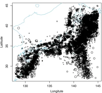
100 km, from 1 January 1965 to 31 December 2009 at magnitudeMJ4.0 and above.

There are 19,019 events in this dataset.Fig. 1shows the epicenter locations of earthquakes used in this study.

Fitting the space–time ETAS to the catalog is not an easy task. For an earthquake catalog covering records over a time period of 38 years, completeness and homogeneity, or the lack thereof, are always problematic in a statistical analysis. For example, when the seismicity in select regions or the whole region has an increasing trend, the fitting results do not converge or converge to unreasonable values. In this study, a target space–time range was chosen so that the seismicity is relatively and visually complete and homogeneous above 4.0 (seeTable 1). The author will investigate seismicity clustering

(9)

Fig. 1. Earthquake locations in the JMA catalog. The different sizes of circles represent earthquakes of different magnitudes fromMJ4.0 to 9.0.

patterns in this polygonal area. In order to compute the weighted likelihood function, the author chooses a two-dimensional step-wise kernel function:

h

(

x

,

y

)

=



k

Wk1Rk

(

x

,

y

),

(25)

whereRiare disjoint octagon rings centered at

(

0

,

0

)

that are formed by the areas between octagons



i

−

1 2 cos j

π

4

,

i

−

1 2 sin j

π

4



:

j

=

0 to 7



and



i 2cos j

π

4

,

i 2sin j

π

4



:

j

=

0 to 7



,

as shown inFig. 2. Here,Wi

=

0

.

6i−1fori

=

1

, . . . ,

8 andWi

=

0 fori

≥

9. LetL

(

T

,

Rk

)

be the

likelihood for the observations in the space–time rangeT

×

Rk. The weighted likelihood is given by

logWL

(

x∗

,

y∗

)

=



k

WklogL

(

T

,

Rk

+ {

(

x∗

,

y∗

)

}

),

(26)

whereL

(

T

,

Rk

+

(

x∗

,

y∗

))

is the likelihood for the observations on the space–time rangeT

×

(

Rk

+

{

(

x∗

,

y∗

)

}

)

. This simplifies the implementation since the algorithm for calculating the integral of the conditional intensity in a polygon is already implemented (Ogata, 1998).

The weighted likelihood estimator is applied so that

(

x∗

,

y∗

)

runs over a fine grid of size 0

.

25°

×

0

.

25°in the polygon region specified inTable 1.Fig. 4gives the background seismicity. A similar background rate was obtained by Zhuang et al.(2004) and Zhuang (2011, 2012) using a semi-parametric estimation method and a space–time ETAS with a nonhomogeneous background rate, and byOgata et al.(2003a) andOgata(2011) using Bayesian estimates for a hierarchical space–time ETAS model with a smoothness prior. FromFig. 3, one can see that the background is the highest around the offshore areas of the Tohoku (northeast) and Hokkaido regions. The western coastal regions and offshore areas are much lower than the highest areas, but still higher than the mid ranges of the main islands. The background intensity is important since it represents the long-term potential of the occurrence of individual earthquake clusters. Together with the clustering parameters, the background seismicity can be used to evaluate future seismicity risks, especially the maximum magnitude in a particular region (seeZhuang, 2012for details).

(10)

Fig. 2. Kernel functionh(x,y)used in the analysis.

Fig. 3. Tectonic settings in the Japan region. EU/AR, NA/OH, PH, and PA represent the Eurasian/Amour, North American/

Okhotsk, Philippine, and Pacific plates, respectively.

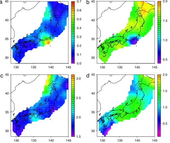
Fig. 5shows how parametersA,

α

,q, and

γ

vary in space. The Izu peninsular and Tonankai regions (southeast to Honshu island) are marked by highAparameter values and low

α

parameter values, which indicates that the clustering behavior of seismicity in these regions is more swarm like, i.e., the numbers of events in each earthquake cluster are similar and do not depend on the magnitude of initial events. The other regions show high

α

(

≥

1

.

2

∼

2) and lowA(0

.

1

∼

0

.

5) values, implying

(11)

Fig. 4. Background seismicity rateµ(unit: events·day−1_·_deg−2_{) estimated using the maximum weighted likelihood.}

a

c

d

b

(12)

Fig. 6. Spatial variation of parameterp(left panel) and distribution map of volcanoes and volcanic arcs in Japan based onSimkin and Siebert(1994) (right panel).

that the earthquake clusters are more (foreshock–)mainshock–aftershock sequences, i.e., a large event (mainshock) comes with abundant aftershocks, which are much smaller than the mainshock. This phenomena is slightly more significant in the Hokkaido and the Shikoku–Nankai regions. The values ofqindicate how the aftershock rate decays in space; high values (above 2.0) are observed in the northwest coastal regions and the region between Shikoku island and the Kei peninsula, compared to lower values of 1.5 to 2 in the other regions. The value of

γ

is approximately 1.0 to 1.7 in most of the study region, with a value lower than 0.7 in the north end of the Ryukyu trough and some parts of the northwest off regions in the Japan sea. Compared toFig. 3, these parameters reflect the spatial tectonic differences among different parts in this region; in particular, the quadruple junction between the Pacific, Philippine, North American/Okhotsk, and Eurasian/Amour plates is characterized by highAand low

α

values.

Fig. 6gives the spatial variation of the parameterp, which measures how the aftershock activity decays in time. One can see that low values ofpexist along the middle tectonic line of Honshu island, which is the same as the volcanic front, whilepincreases off this line. Similar patterns were obtained byUtsu(1969) andOgata(2004) using different approaches.

The spatial variations of parameterscandDare not discussed herein since they are influenced by the missing small aftershocks immediately after the mainshock and location errors, respectively.

5. Summary

In this article, based on the theory of residual analysis for point processes, the weighted likelihood estimator was proposed and applied to the space–time ETAS model to study the spatial variation of clustering features of seismicity patterns in the Japan region. From the analysis results, one can see that the weighted likelihood estimators for point processes are useful for exploring how a model changes spatially, temporally, and spatiotemporally, i.e., to detect the spatial and temporal variations of model parameters. This is especially useful when observational data is obtained under a complex or changing environment. In the application example, the spatial variations of the MWLEs of each ETAS parameter showed different features for different tectonic regions. For example, lowp-value regions corresponded to volcanic zones, and the convergence of the Eurasian, Philippine, and Pacific plates was characterized by low

α

, highA, and highpparameter values. Revealing the spatial variations of the ETAS parameters is helpful for issuing high-resolution probability forecasting of regional seismicity. The proper choices of the optimal kernel function and bandwidth were not discussed in this study; however, the author plans to investigate these issues in future research.

(13)

Acknowledgment

The author is partially supported by Grants-in-Aid No. 2530052 for Scientific Research (C) from the Japan Society for the Promotion of Science.

References

Baddeley, A., Turner, R., Møller, J., Hazelton, M.,2005. Residual analysis for spatial point processes (with discussion). J. R. Stat. Soc. Ser. B Stat. Methodol. 67 (5), 617–666.

Besag, J.,1975. Statistical analysis of non-lattice data. The statistician 179–195.

Bray, A., Schoenberg, F.P.,2013. Assessment of point process models for earthquake forecasting. Statist. Sci. 28 (4), 510–520. Bray, A., Wong, K., Barr, C.D., Schoenberg, F.P.,2014. Voronoi residual analysis of spatial point process models with applications

to california earthquake forecasts. Ann. Appl. Stat. 8 (4), 2247–2267.

Console, R., Murru, M., Lombardi, A.M.,2003. Refining earthquake clustering models. J. Geophys. Res. 108 (B10), 2468. Daley, D.D., Vere-Jones, D.,2003a. An Introduction to Theory of Point Processes – Volume 1: Elementrary Theory and Methods,

second ed.. Springer, New York, NY.

Daley, D.D., Vere-Jones, D.,2003b. An Introduction to Theory of Point Processes - Volume II: General Theory and Structure, second ed.. Springer, New York, NY.

Guan, Y., Shen, Y.,2010. A weighted estimating equation approach for inhomogeneous spatial point processes. Biometrika 97 (4), 867–880.

Guan, Y., Waagepetersen, R., Beale, C.M.,2008. Second-order analysis of inhomogeneous spatial point processes with proportional intensity functions. J. Amer. Statist. Assoc. 103 (482), 769–777.

Helmstetter, A., Kagan, Y.Y., Jackson, D.D.,2005. Importance of small earthquakes for stress transfers and earthquake triggering. J. Geophys. Res. 110.

Jalilian, A., Guan, Y., Waagepetersen, R.,2013. Decomposition of variance for spatial cox processes. Scand. J. Stat. 40 (1), 119–137. Møller, J., Schoenberg, F.P.,2010. Thinning spatial point processes into Poisson processes. Adv. Appl. Probab. 42 (2), 347–358. Møller, J., Waagepetersen, R.P.,2003. Statistical Inference and Simulation for Spatial Point Processes. Chapman and Hall/CRC. Ogata, Y.,1988. Statistical models for earthquake occurrences and residual analysis for point processes. J. Amer. Statist. Assoc.

83, 9–27.

Ogata, Y.,1998. Space–time point-process models for earthquake occurrences. Ann. Inst. Statist. Math. 50, 379–402. Ogata, Y.,2011. Significant improvements of the space–time ETAS model for forecasting of accurate baseline seismicity. Earth

Planets Space 63 (3), 217–229.

Ogata, Y.,2004. Space–time model for regional seismicity and detection of crustal stress changes. J. Geophys. Res. 109 (B3), B03308.

Ogata, Y., Jones, L.M., Toda, S.,2003a. When and where the aftershock activity was depressed: Contrasting decay patterns of the proximate large earthquakes in southern California. J. Geophys. Res. 108, B62318.

Ogata, Y., Katsura, K., Tanemura, M.,2003b. Modelling heterogeneous space–time occurrences of earthquakes and its residual analysis. J. R. Stat. Soc. Ser. C. Appl. Stat. 52 (11), 499–509.

Ogata, Y., Zhuang, J.,2006. Space–time ETAS models and an improved extension. Tectonophysics 413 (1–2), 13–23. Schoenberg, F.P.,2003. Multidimensional residual analysis of point process models for earthquake occurrences. J. Amer. Statist.

Assoc. 98 (7), 789–795.

Schoenberg, F.P.,2005. Consistent parametric estimation of the intensity of a spatial–temporal point process. J. Statist. Plann. Inference 128, 79–?3.

Simkin, T., Siebert, L.,1994. Volcanoes of the World. Geoscience Press, Tucson, Arizona.

Sornette, D., Werner, M.J.,2005a. Apparent clustering and apparent background earthquakes biased by undetected seismicity. J. Geophys. Res. 110, B09303.

Sornette, D., Werner, M.J.,2005b. Constraints on the size of the smallest triggering earthquake from the epidemic-type aftershock sequence model, Båth’s law, and observed aftershock sequences. J. Geophys. Res. 110 (B08304).

Utsu, T.,1969. Aftershock and earthquake statistics (i): Some parameters which characterize an aftershock sequence and their interrelations. J. Fac. Sci., Hokkaido Univ. 3, 129–195. (Ser. VII (Geophysics)).

Utsu, T., Ogata, Y., Matsu’ura, R.S.,1995. The centenary of the Omori formula for a decay law of aftershock activity. J. Phys. Earth 43, 1–33.

Vere-Jones, D., Schoenberg, F.P.,2004. Rescaling marked point processes. Aust. N. Z. J. Stat. 46 (1), 133–143.

Waagepetersen, R.P.,2007. An estimating function approach to inference for inhomogeneous neyman-scott processes. Biometrics 63 (1), 252–258.

Zhuang, J.,2006. Second-order residual analysis of spatiotemporal point processes and applications in model evaluation. J. R. Stat. Soc. Ser. B Stat. Methodol. 68 (4), 635–653.

Zhuang, J.,2011. Next-day earthquake forecasts by using the ETAS model. Earth, Planet, and Space 63, 207–216.

Zhuang, J.,2012. Long-term earthquake forecasts based on the epidemic-type aftershock sequence (ETAS) model for short-term clustering. Res. Geophys. 2 (1), e8.

Zhuang, J., Chang, C.-P., Ogata, Y., Chen, Y.-I.,2005. A study on the background and clustering seismicity in the Taiwan region by using a point process model. J. Geophys. Res. 110, B05S13.

Zhuang, J., Ogata, Y.,2006. Properties of the probability distribution associated with the largest event in an earthquake cluster and their implications to foreshocks. Phys. Rev., E 73.

Zhuang, J., Ogata, Y., Vere-Jones, D.,2002. Stochastic declustering of space–time earthquake occurrences. J. Amer. Statist. Assoc. 97 (3), 369–380.

Zhuang, J., Ogata, Y., Vere-Jones, D.,2004. Analyzing earthquake clustering features by using stochastic reconstruction. J. Geophys. Res. 109 (3), B05301.