w o r k i n g
p
a
p
e
r
F E D E R A L R E S E R V E B A N K O F C L E V E L A N D
09
13
The Long Run Effects of Changes in
Tax Progressivity
Working papers
of the Federal Reserve Bank of Cleveland are preliminary materials circulated to
stimulate discussion and critical comment on research in progress. They may not have been subject to the
formal editorial review accorded offi cial Federal Reserve Bank of Cleveland publications. The views stated
herein are those of the authors and are not necessarily those of the Federal Reserve Bank of Cleveland or of
the Board of Governors of the Federal Reserve System.
Working papers are now available electronically through the Cleveland Fed’s site on the World Wide Web:
Working Paper 09-13
December 2009
The Long Run Effects of Changes in Tax Progressivity
by Daniel R. Carroll and Eric R. Young
This paper compares the steady state outcomes of revenue-neutral changes to the
progressivity of the tax schedule. Our economy features heterogeneous
house-holds who differ in their preferences and permanent labor productivities, but it
does not have idiosyncratic risk. We fi nd that increases in the progressivity of
the tax schedule are associated with long-run distributions with greater
aggre-gate income, wealth, and labor input. Average hours generally declines as the
tax schedule becomes more progressive implying that the economy substitutes
away from less productive workers toward more productive workers. Finally, as
progressivity increases, income inequality is reduced and wealth inequality rises.
Many of these results are qualitatively different than those found in models with
idiosyncratic risk, and therefore suggest closer attention should be paid to
model-ing the insurance opportunities of households.
Key words: heterogeneity, progressive taxation, complete markets.
JEL codes: E21, E25, E62
Daniel R. Carroll is at the Federal Reserve Bank of Cleveland and can be reached
at [email protected]. Eric R. Young is at the University of Virginia and can be
reached at [email protected].
1. Introduction
The purpose of this paper is to study the effects of flattening progressive tax functions when markets for insurance are complete. The literature on the gains from flattening the tax code is large – some recent quantitative examples include Ventura (1999), Casta˜neda, D´ıaz-Gim´enez, and R´ıos-Rull (1999), D´ıaz-Gim´enez and Pijoan-Mas (2006), Conesa and Krueger (2006), and Conesa, Kitao, and Krueger (2008). All of these papers begin with the presumption that insurance markets are absent (as in Aiyagari 1994); progressive taxation therefore has beneficial insurance properties, as it reduces the variance of labor income.1 It turns out that a robust prediction of these models is
that aggregate activity and welfare respond positively to ”flattening” the tax code. In contrast, we approach the problem from the other end of the spectrum – we ask how progressive tax reform would effect the economy in a model without any uncertainty where inequality is entirely due to immutable heterogeneity in preferences and endowments.
Constructing a model that matches the US distributions of income and wealth not based on idiosyncratic risk is difficult given the results we found in Carroll and Young (2009). In the absence of discount factor heterogeneity, deterministic models with progressive taxation predict that the stationary distribution will have a negative correlation between income and wealth and between capital and labor income, both of which are inconsistent with US data.2 To get around these problems, we construct distributions of discount factors, labor productivities, and labor supply disutilities that exactly match the distributions of assets, income, and labor hours in the model to those in the data. We use this model to investigate the response of the economy to changes in the progressivity of the income tax code.3
1Meh (2005) considers how progressive taxation affects the economy in a world with risky saving via entrepreneurial
activity.
2
Elastic labor supply and/or borrowing constraints do not affect those results.
3
The qualitative and quantitative implications of tax reforms in our model are quite different than those in the incomplete market literature. We conduct three revenue-neutral tax reform experiments and find that flattening the tax code – reducing the progressivity of the income tax – tends to reduce aggregate capital and labor input, rather than increase it; the decrease is also quantitatively large. More progressive marginal tax schedules can lead to steady states with as much as 47% and 40% greater aggregate capital and labor input, respectively. The results of our other experiments, though less pronounced, consistently find that tax reforms with more progressive schedules have increase aggregate capital and labor input. We also find that increased progressivity generally decreases income inequality and increases wealth inequality. These changes occur without any change in the average tax rate in the economy, since we impose revenue neutrality on our experiments. With respect to labor input, progressivity increases labor input because it reallocates labor from less productive to more productive agents, generating output gains even though labor supply – measured by raw hours – actually declines.
Our results have two implications. First, endogenizing the extent to which the private sector can provide insurance – as in Krueger and Perri (2005) or ´Abrah´am and Carceles-Poveda (2007) – may be critical for understanding whether progressive taxation increases or decreases aggregate activity. Second, the extent to which inequality is driven by preferences vs. endowments also will play a role in determining the effects of progressive taxation, as they do in determining the effects of eliminating the business cycle (see Krusellet al. 2009).
2. Model
The model economy is composed of three sectors: a stand-in firm, a government, and a collection of heterogeneous households.
2.1. Households
The economy is populated by an infinite set I of households of unit measure. These households differex ante along three dimensions: their discount factor β, their permanent labor productivity
ε, and their disutility from labor B. Every household is endowed with 1 unit of discretionary time which it may allocate to leisure, ℓ, or labor, h. Any household i ∈ I has preferences over consumption,c, and leisure which are described by the following lifetime utility function:
Ui = ∞ X t=0 βti log (cit) +Bi ℓ1it−σ 1−σ . (2.1)
σ ≥ 0 is the inverse of the Frisch elasticity of leisure and is assumed uniform across households.4
While we do not focus on sustained growth, the utility function is consistent with a balanced-growth path along which leisure and labor supply are constant.
2.2. Firm
Each period, a stand-in firm uses capital and labor input to produce output according to a pro-duction technology F(K, N). Let F(K, N) be strictly concave and increasing in K and N and
F(0, N) = F(K,0) = 0. Output may be consumed or invested toward future capital. The firm rents inputs from the households through perfectly competitive markets. Letting the production technology be Cobb-Douglas with capital share parameter α ∈ [0,1], profit-maximization implies that each input is paid its marginal product so
rt = F1(K, N) =αKα−1N1−α wt = F2(K, N) = (1−α)KαN−α. 4
We assume that each period the stock of capital depreciates by a factor δ∈[0,1].
2.3. Government
Each period, the government collects revenue from a tax on income, τ(y) and purchases Gt goods which do not enter the households’ utility functions. Let τ′(y) : R
+ → [0,1) be continuous
and monotone increasing. Let Γ (i) be the density of agents over typesi. Any surplus revenue is rebated back to the households via a lump-sum transfer, Tt, so that the government’s budget constraint,
Tt=
Z
τ(yit) Γ (i)di−Gt (2.2)
is satisfied each period. We abstract from the presence of government debt.
2.4. Equilibrium
Each household i maximizes (2.1) by choice of consumption, leisure, and savings, ki,t+1, while
respecting its budget and time constraint
cit+ki,t+1 = yit−τ(yit) +Tt+kit (2.3)
ℓit+hit ≤ 1 (2.4)
where
yit=wtεihit+ (rt−δ)kit (2.5)
is household income. Given the behavior of the firm and the government and a population density Γ (i), an equilibrium can be defined as a set of household decisions
{cit, ℓit, ki,t+1}∞t=0 iεI,, market prices{wt, rt}∞t=0, and government policies {Gt, Tt}∞t=0 such that for anyt∈ {0,1, ...}
2. {wt, rt} clear the labor and capital markets: Kt = Z kitΓ (i)di Nt = Z hitεiΓ (i)di.
3. The goods markets clear:
Z citΓ (i)di + Z ki,t+1Γ (i)di +Gt=F(Kt, Nt) + (1−δ)Kt.
4. At {Gt, Tt} the government’s budget is balanced.
The household’s optimization problem has a continuous, concave objective function and a com-pact and convex constraint set. Along with (2.3) and a transversality condition for each i∈I, the following system of equations describes an equilibrium:
ci,t+1 cit = βi 1 + 1−τ′(yit) (rt−δ) (2.6) 0 ≥ 1 cit 1−τ′(yit) wtεi−Bi(1−hit)−σ; (2.7)
2.5. Steady State
Equations (2.6), (2.7), (2.3), and (2.5) simplify in the steady state to
1 = βi1 + 1−τ′(yi) (r−δ) (2.8) 0 ≥ 1 ci 1−τ′(yi) wεi−Bi(1−hi)−σ with eq. ifhi>0 (2.9) ci = yi−τ(yi) +T (2.10) yi = wεihi+ (r−δ)ki. (2.11)
For a given rental rate, (2.8) pins down the long-run marginal tax rate for each household. Since
τ′(y) is strictly increasing, each marginal tax rate is associated with a unique level of income, and (2.8) identifies the long-run distribution of income. Givenτ′(y), household i’s long-run income is a function only ofβi and r:
yi βi, r;τ′ = τ′−1 1− β −1 i −1 r−δ =θ βi, r;τ′ . (2.12)
Note the following properties ofθ: ∂β∂θ >0, ∂θ∂r >0, and ∂τ∂θ′ <0.
Because for a given tax function and transfer, a household’s steady state consumption depends only upon its income, the hours supplied by a household can be expressed as a function of its preferences and market prices:
hi βi,Bi εi , r;τ′ = 0 ifAi> Bεii 1−AiBεii 1σ otherwise where Ai = c(θ(βi, r;τ′)) [1−τ′(θ(β i, r;τ′))]w = θ(βi, r;τ ′)−τ(θ(β i, r;τ′)) +T hβ−1 i −1 r−δ i w .
Hours have not been expressed as a function of the wage because equilibriumw can be written as a function of r and α under the assumptions about F. Note that what matters for hours is not productivity per se, but rather productivity relative to the disutility parameter.
Finally, the long run wealth of each household is also determined by preferences and prices through (2.11), so ki βi,Bi εi , εi, r;τ′ = θ(βi, r;τ′)−wε ihi βi,Bi εi, r;τ ′ r−δ .
The level of productivity plays a role in determining the asset holdings of each household.
2.5.1. The role of household characteristics on steady state income, wealth, and hours Holding market prices and government policy fixed, we now examine how long run income, wealth and hours are affected byβi,εi, and Bi.
• The Discount Factor: Given market prices, βi identifies long run income yi. Larger β implies larger y. Turning to hours and wealth,
∂h ∂β = − 1 σ Ai Bi εi σ1−1 Bi εi 1−∂τ∂θ ∂θ ∂β β−1 −1 r−δ w+ (θ−τ(θ) +T) w β2 (r−δ) β−1 i −1 r−δ 2 w < 0 and ∂k ∂β = 1 r−δ ∂y ∂β −wε ∂h ∂β >0.
More patient households will save more and work less, all other things equal.
consumption. For hours and wealth, ∂h ∂ε = 1 σ (AiBi) 1 σ ε− 1 σ−1>0 and ∂k ∂ε =− wε r−δ ∂h ∂ε − wh r−δ <0
so hours rise withεand wealth declines.
• Disutility of Labor: As one would expect, increases inB decrease steady state hours and increase steady state wealth.
• Frisch Elasticity: The parameterσ (the reciprocal of the Frisch elasticity) only affects the sensitivity of the responses of hours and wealth, not the direction. As σ → ∞, h∗ → 1, so that hours and wealth are unresponsive to changes in either parameters or prices.
2.5.2. The response of steady state income, wealth, and hours to changes in prices and fiscal policy
To better understand our numerical results, it is helpful to do some partial equilibrium comparative statics on the steady state.
• Increase in τ(yi) (or a decrease in T):
Holding prices fixed, an increase inτ(yi) (or a decline inT) does not affect long run income;
Ai falls. Hours weakly rise for each household not at the lower bound on hours after the Ai decrease.5 Wealth moves in the opposite direction as hours so it weakly falls.
• Increase in τ′(y i): 5
If the marginal tax rate rises, then according to (2.8) yi falls. For households with discount factors not less than 1+1r−δ, hours weakly rise in response to an increase in the marginal tax rate. ∂h ∂τ′ = − 1 σ Ai Bi εi σ1−1 Bi εi 1−∂τ ∂θ (θ) ∂θ ∂τ′ hβ−1 i −1 (r−δ) i w = −1 σ Ai Bi εi σ1−1 Bi εi ∂θ ∂τ′ w > 0,
where the second equality is true because
∂τ
∂θ (θ) = 1−
β−i 1−1
r−δ
by (2.12). Less patient households will already be converging to the natural borrowing limit where hours approach 1. Decreasing the return to savings by increasing their marginal tax rate will not induce them to reverse their behavior. Therefore as long as β is sufficiently large, steady state wealth decreases with τ′.6
• Increase inr (decrease inw): An increase in the steady state rental rate (or equivalently a decline in the aggregate wage) leads to a rise in income for every household. The size of this increase for any given household will depend upon what part of the marginal tax function the household faces. In order for (2.8) to be satisfied, for any household i the after-tax return on savings in the new steady state must be equal to what it was in the initial steady state. Therefore an r increase must be offset by an increase in τ′(yi) (i.e., yi must increase). If a 6
In our experiments no household has aβless than 1 1+r−δ.
particular household is in a region of the marginal tax function where its derivative is near zero (near the upper bound), then a large increase inyi will be necessary to satisfy (2.8). On the other hand if the derivative is large, then only a small increase inyi will restore equality in (2.8). Therefore, an increase inr will tend to increase income inequality. In addition, the long run response of hours is negative and therefore that of wealth is positive.
3. Numerical Experiments
In order to find quantitative results for the model, we conduct a series of revenue neutral tax experiments. We select the following functional form for each household’s tax bill:
τ(y) =ν0 y− y−ν1 +ν 2− 1 ν1 +ν3y.
The first term is the functional form Gouveia and Strauss (1994) assumed to estimate the effective personal income tax function using 1989 US tax return data.7 The second term, ν3y, captures
other tax revenues that are not modeled but are paid by households in the data (e.g., excise taxes, estate taxes, property taxes). In the interest of focusing on the progressivity of the personal income tax, the combined effect of these other taxes is assumed to be a linear function of income. ν0 sets
the upper bound on the marginal personal income tax rate. The highest possible value of τ′(y) then is ν0 +ν3. ν1 changes the curvature of the function. The exact way in which it does so
will be clear after the first experiment. Finallyν2 adjustsτ(y) for the unit of measure of income.
Throughout all experiments its value remains fixed. It is important to remember that because of revenue neutrality, the average tax rate is unchanged across experiments. The wide range of
7
This functional form has been used in a number of quantitative studies of progressive taxation, including Casta˜neda, D´ıaz-Gim´enez, and R´ıos-Rull (1999), Conesa and Krueger (2006), and Conesa, Kitao, and Krueger (2008). An alternative smooth specification is used in Sarte (1997), Li and Sarte (2003), and Carroll (2009), while a more detailed nonsmooth function is used in Ventura (1999).
steady state distributions and of their corresponding moments strongly suggests that ignoring the distributional effects of tax changes may not be innocuous.
3.1. Calibration
To initialize the model, we calibrate to income, wealth, hours, and analysis weight data from the Survey of Consumer Finances 1992, 1995, 1998, 2001, and 2004. The total number of households used for the experiment is 15,437. After deflating these data by the 1992 GDP deflator, we normalize aggregate income to 1, wealth to 3, and hours to 0.33. We set α = 0.36 and σ = 2. Government spending is 20 percent of aggregate income and transfers are 10 percent. We also fix
ν0 and ν1 to 0.258 and 0.768 from Gouveia and Strauss (1994).We set the remaining parameters
so that the steady state of our model matches specific aggregate statistics at the annual frequency.
ν3 = 0.0855 which implies that 71.5% of tax revenue is raised through the progressive personal
income tax.8 Depreciation is set toδ = 0.05 so that investment is 15 percent of income. ψi for each household is set to the household’s population weight in the SCF. We then normalize these weights so that P
ψi = 1.
{βi, εi, Bi},r, andν2 are solved for jointly. The preference parameters are backed out from the
first-order conditions and definition of income for each household. A difficulty with this method arises when a survey household works zero hours. Because the intratemporal condition is not binding there are infinitely many possible solutions to the system. Specifically, it is impossible to back outεi andBidirectly. To address this problem, we first solve for the household characteristics of working households and regress in logs εi on age, education, and race (reported in the survey). In addition, we construct the cdf ofB. Then if we encounter a non-working household, we use its
8
This is the average fraction of tax revenue from personal income taxes for the years 1992−2004. Our measure
is taken from the Office of Management and Budget Historical Table 2.2. We do not include Social Insurance and Retirement Receipts in our calculation, so we exclude FICA taxes.
reported age, education, and race along with the regression equation to get a predicted εi. Given
εi, we find Bi,min for which the intratemporal condition just binds. To select a Bi we draw from the cdf of B truncated below at Bi,min. Finally, r and ν2 are adjusted to clear the market for
capital goods and the government budget constraint.
3.1.1. A note on the measurement of tax progressivity
We now discuss the notion of progressivity. It is not clear exactly how to characterize a tax change as ”progressive” or ”regressive” when the underlying distribution of income changes. As a result, it is not straightforward to compare the progressiveness of two tax functions and so there are several methods used in the literature, and these measures may not agree on the ranking of tax schedules. We choose to report the Kakwani (1977) index which is the tax Gini coefficient minus the income Gini coefficient. A higher value of the index corresponds to greater progressivity. This index is particularly well-suited to our problem because the income distribution is not fixed in our experiments. To see this, suppose two tax functions, τA and τB, are associated with two different steady state income distributions ΓA and ΓB, and without loss of generality assume that
GτA > GτB, where Gτi is the Gini coefficient of the tax burden in the steady state resulting from
τi. In words, the tax burden in steady stateAis more unequal than it is inB. Now there are two possible reasons for why this may be the case. First,τAmay simply place higher average tax rates on high income households thanτB. Alternatively, ΓAmay have a greater fraction of high income households than ΓB so that most of the tax burden rests with these high income households (even if their average rate is lower than under τB). The Kakwani index corrects for these differences in income inequality.
In Tables 2, 4, and 6, we report the Gini coefficients of income and of wealth as well as two Kakwani index calculations. Because it is not certain that a tax change which seems more
pro-gressive initially will end up being more propro-gressive in resulting steady state, we give two Kakwani index measures. Kakpre measures the Kakwani index of the tax change using the initial income distribution, whileKakpost measures the index on the long run distribution of income. In our ex-periments, the direction of progressivity never reverses (i.e., the ordering of tax reforms according to progressivity resulting from Kakpre is preserved under Kakpost). Nevertheless, in most cases the degree of progressivity is significantly diminished in the long run as households respond to the new tax code. Kakpost > Kakpre in only the final experiment, and this occurs because the Gini coefficient of the tax burden hits its upper bound of 1 while income inequality increases in the new steady state.
3.1.2. Experiment 1: Increase in the Curvature of the Personal Income Tax
In this experiment we increase the value of v1 and adjust ν3 to balance the government budget
constraint. v1 alters the degree of progressivity of the tax function: when v1 = 0 the personal
income tax is flat, but when ν1 > 0, average tax rates and marginal tax rates rise with income.
Figure 1 displays the marginal personal income tax function for several ν1 values in the range
explored in the experiment. A higherν1 reduces the marginal tax rate on low incomes and induces
a more rapid rise to the highest rate, ν0.9 This figure, however, does not account for revenue neutrality’s effect on the total tax bill. Figure 2 shows the marginal tax bill function which reflects the changes both in ν1 and ν3. When revenue neutrality is imposed it is not immediately clear which tax is more progressive. Aν1 of 0.768 places a higher total marginal tax rate on low income
than greater ν1 values do. Compared to a value of 2.0,ν1 = 3.0 leads to higher marginal tax rates
on high income households as one would expect, but it also imposes higher rates on the very poor. Turning to the effects of tax policy changes on the long-run levels of aggregate variables. We 9In the limit as
ν1→ ∞, the marginal tax function approaches a flat tax with an exemption at low income levels.
report the percentage changes in the aggregates in Table 1. ν1 has a hump-shaped relationship
with income, capital, labor input, and wages. Figure 3 plots the steady state levels of aggregate income, capital and consumption over ν1. All three exhibit dramatic responses to changes inν1. For example, increasing ν1 from 0.768 to 2.0 causes aggregate wealth to increase by 46.8 percent.
Even at the highest value of ν1, capital is still 43 percent above the baseline level. Responses
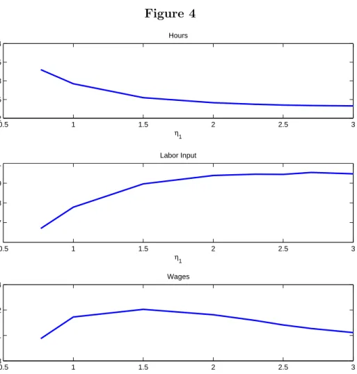
in the labor market are plotted in Figure 4, average hours decline by as much as 29.4 percent meaning that higher progressivity in the personal income tax causes a substitution in production from less-productive to more-productive households. Interestingly, this pattern persists at high values ofν1 even though the average wage falls sharply in this region. The large increase in labor
input comes from the upper 4 percent of productive households. Figures 5 and 6 plot the average hours within each percentile of theε-distribution for the baseline andν1 = 2.0 cases. Notice that
hours fall for nearly the entire economy, however, they rise somewhat at the upper end. Clearly average hours fall, but the impact on labor input of the upper 4 percent is much more significant. To make this more pronounced, we plot the average labor input within each percentile of ε. This is shown in Figures 7 and 8. Now the difference at the upper tail is starkly apparent, especially in the top 1 percent.
One advantage of the modeling technique used here is the ability to characterize behavior at the extremes of the income and wealth distributions. Figures 9 and 10 show the breakdown in income, wealth and consumption across the steady state distribution for some values ofν1. There
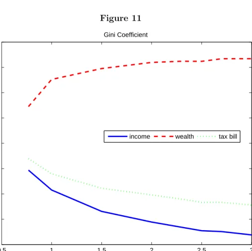
are several conclusions that can be made about ν1 increases. First, increasingν1 reduces income inequality. The Gini coefficient of income is cut by more than 50 percent whenν1 increases from
its baseline to 3.0. In general this is caused because low and middle-income households marginal total tax rates are reduced the most. Nevertheless, not all high income households reduce their income. Finally, the interest rate is lower in the ν1 = 3.0 steady state. As discussed previously,
this leads to lower income inequality. Wealth inequality, on the other hand, increases. Plots of the income, wealth, and tax burden Gini coefficients across steady states is shown in Figure 11.
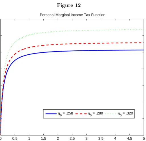
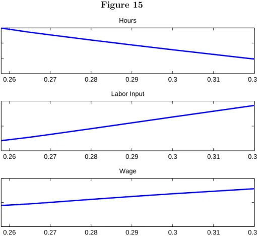
3.1.3. Experiment 2: Shift between Personal Income Taxation and other Tax Sources This experiment increases the fraction of tax revenue raised with the progressive income tax rel-ative to the flat tax by increasing ν0 and reducing ν3. Figures 12 and 13 compare the baseline
marginal personal income tax functions and marginal tax bill functions for several values ofν0 in
the experiment.10 As ν0 increases the marginal personal tax function rotates upward, however the marginal total tax function rotates downward which is consistent with our finding from the previous experiment that higher progressivity is associated with more aggregate activity. In fact, in the steady state where ν3 = 0, aggregate income is 11.6 percent larger and the capital stock is 14.5 percent larger than in the baseline case. Percent changes for all aggregates are displayed in Table 3. In figures 14 and 15, the steady state values of the economy’s aggregates are plotted for the whole range of ν0 in the experiment. There is basically a linear relationship between ν0
and the aggregate variables. As in experiment 1 (though to a lesser degree), average hours falls and total labor input rises so once again more progressivity is effecting a substitution from less productive workers to more productive workers.
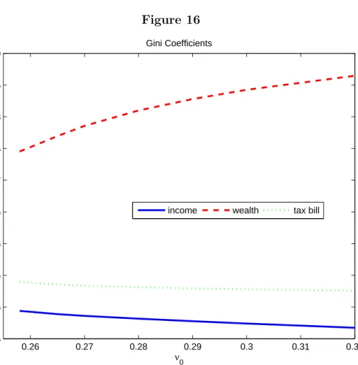
The qualitative results for inequality are also similar to those from experiment 1. Figure 16 plots the steady state Gini coefficients of income, wealth, and taxes. The income Gini falls slightly as the total tax schedule tilts towards the progressive income tax schedule. In contrast, wealth inequality rises significantly (roughly 16%). In this case, the large increase in wealth inequality comes primarily from large negative asset positions taken by moderately patient households with very high labor productivity.
10At
3.1.4. Experiment 3: Flat Tax with an Exemption
In our final experiment, we consider a tax function like that from Conesa and Krueger (2006) who find that the optimal progressive income tax combines a flat tax with an exemption level for income. In our case, this is approximated by lettingν1 → ∞. In keeping with that paper we eliminate the
linear schedule (i.e., ν3 = 0) and adjust ν0 to balance the government’s budget. There are two
marginal tax rates under this system – one is zero and the other isτ =ν0, with a level of income y = 1 that determines the switch.11 Incomes above ¯y pay a tax bill ¯τ∗y¯, while incomes below ¯y
pay nothing.
Proposition 3.1. Given the tax function described above and a set of types each with a discount factor from {β1, β2, ..., βN} where 1 > β1 > β2 > ... > βN >0, in any steady state with positive government expenditures
β2 ≤ 1 + (1−¯τ) (r−δ)
1 +r−δ β1.
Further, any type with discount factor β1 has income y1>1. Types with discount factors less
thanβ2 have income equal to−T. Any type withβ =β2 will havey2 ≤1.
Proof A necessary condition for a steady state is that
1≥βn[1 + (1−τy(yn)) (r−δ)] ∀n (3.1) where τy(y) = 0 if y≤1 ¯ τ >0 if y= 1 . 11
First, from the household’s budget constraint any typenwith assets approaching the borrowing limit must steady state income approaching −T. Thus ifyn>−T,
1 =βn[1 + (1−τy(y)) (r−δ)].
Second, since government expenditures are positive by budget balance τy(y) = ¯τ for at least one type, implying that there are households with income greater than 1 in the steady state. The steady state Euler equation for any such household is
1 =βn[1 + (1−¯τ) (r−δ)]
Given an r and a ¯τ, this condition can only be satisfied for one βn. It is easy to see that this
βn=β1. If it were satisfied for some otherβn, then
1< β1[1 + (1−τy(y)) (r−δ)]
which violates (3.1). Therefore
1 =β1[1 + (1−¯τ) (r−δ)]
and
1> βn[1 + (1−¯τ) (r−δ)], n >1.
Note that (3.1) is satisfied for n >1 when
βn≤ 1 + (1−τ¯) (r−δ)
implying
βn≤ 1
1 +r−δ.
To complete the proof, we will now show that a steady state cannot exist forβn≥ 1+(11+−τ¯r−δ)(r−δ)β1. Assume not. Then there must exist a βs such that
βs =η 1 1 +r−δ + (1−η) 1 1 + (1−¯τ) (r−δ) , 0< η <1. Eitherys≤1 orys>1. If ys≤1, then 1 ≥ βs[1 +r−δ] ≥ η 1 1 +r−δ + (1−η) 1 1 + (1−¯τ) (r−δ) [1 +r−δ] ≥ η(1 + (1−¯τ) (r−δ)) + (1−η) (1 +r−δ) 1 + (1−¯τ) (r−δ) 1 + (1−τ¯) (r−δ) ≥ η(1 + (1−¯τ) (r−δ)) + (1−η) (1 +r−δ) (1−η) (1 + (1−¯τ) (r−δ)) ≥ (1−η) (1 +r−δ)
which is a contradiction because ¯τ >0. Therefore ys>1, and
1 = η 1 1 +r−δ + (1−η) 1 1 + (1−τ¯) (r−δ) [1 + (1−τ¯) (r−δ)] = η[1 + (1−τ¯) (r−δ)] + (1−η) (1 +r−δ) 1 +r−δ 1 +r−δ = η[1 + (1−τ¯) (r−δ)] + (1−η) (1 +r−δ) η(1 +r−δ) = η[1 + (1−τ¯) (r−δ)]
steady state.
Define an intermediate β type as any typenfor which
β1[1 + (1−τ) (r−δ)]
1 +r−δ < βn< β1.
As shown above, the existence of an intermediateβtype rules out a steady state. To see this, note that y = 1 is the the only potential steady state income value for any intermediate β type. At
y = 1, however, consumption growth must be positve because this type discounts the future less than the market pays for deferred consumption (i.e., βn > 1+1r−δ) so income rises. Any increase in income discontinuously increases the marginal tax rate so that the market no longer sufficiently rewards this type for postponing consumption. Consumption growth will be less than one so income will fall. If the number of intermediateβ types is greater than 1, then the most patient of them will have the largest consumption growth in the initial period and will converge the slowest back toward an income of 1.
The wealth distribution in this case would have the most patient type holding the largest share of wealth (possibly an extremely large share). Intermediate β types could have positive or negative wealth depending upon their labor income. All other types have assets approaching the natural borrowing limit. We find that intermediate types exist in our calibrated economy, thus the reported findings for this experiment are not from a steady state. They should be interpreted instead as reporting features of an economy with a joint income and wealth distribution that is the limiting distribution from the sequence of steady states associated with a sequence of ν1, whereν1
approaches infinity.
In the steady state of our numerical experiment, τ = 14.5 percent. Table 5 reports the per-centage changes in the steady state aggregates. Aggregate income rises by 203 percent while the
capital stock increases by 266 percent. The extreme rise in these values is caused almost entirely by the behavior of the most patient household. This household has income equal to 40,672 times the average and wealth equal to 166,512 times the average.12 Hours increase only 11 percent, but total labor input surges by 185 percent. The big increase in labor input is not caused by the most patient household but rather by the highly productive among the other households. Hours for these households rise in response to a zero tax rate, leading to large increases in labor income. To maintain an income level below y, this additional labor income is balanced by very large negative asset positions. With households in this economy taking such extreme positions, it is not surprising that inequality increases significantly. The Gini coefficient of income rises by 41.4 percent to 0.7, and the Gini coefficient of wealth rises from 0.745 to nearly 1.
4. Conclusion
In this paper we have investigated the consequences of altering the progressivity of the tax code in a model with heterogenous household but no idiosyncratic risk. As we noted in the Introduction, our results are qualitatively different from those found in models with incomplete asset markets. Thus, we argue that more attention must be paid to deriving the insurance opportunities available to households, either in terms of borrowing limits or missing insurance markets. Some papers take steps in this direction, such as Krueger and Perri (2005) or ´Abrah´am and Carceles-Poveda (2007), but more work is needed. Table 7 illustrates how assumptions about the nature of income and wealth inequality lead to different predictions about the effects of flattening the tax code.
We want to point out ”progressive” tax reforms – that is, changes in the tax function that induce more progressivity relative to the estimated U.S. tax function – would enjoy strong political
12
To give some perspective to this number, the average wealth in the US is around $180,000 (inclusive of illiquid retirement portfolios and housing). Our wealthiest household therefore has a wealth of nearly $30 billion. Currently there are only 3 individuals on the Forbes’s billionaires list with total wealth greater than this.
support. Carroll (2009) contains an investigation of the source for this support; it would be of considerable interest to investigate this issue in the models that endogenize risk sharing.
References
[1] ´Abrah´am, ´Arp´ad and Eva Carceles-Poveda (2007), ”Tax Reform with Incomplete Markets and Endogenous Borrowing Limits,” manuscript.
[2] Aiyagari, S. Rao (1994), ”Uninsured Idiosyncratic Risk and Aggregate Saving,” Quarterly Journal of Economics 109(3), pp. 659-684.
[3] Becker, Robert A. (1980), ”On the Long-Run Steady State in a Simple Dynamic Model of Equilibrium with Heterogeneous Households,” Quarterly Journal of Economics 95(2), pp. 375-382.
[4] Carroll, Daniel R. (2009), ”The Demand for Income Tax Progressivity in the Growth Model,” manuscript.
[5] Carroll, Daniel R. and Eric R. Young (2009), ”The Stationary Distribution of Wealth under Progressive Taxation,”Review of Economic Dynamics 12(3), pp. 469-478.
[6] Casta˜neda, Ana, Javier D´ıaz-Gim´enez, and Jos´e-V´ıctor R´ıos-Rull (1999), ”Earnings and Wealth Inequality and Income Taxation: Quantifying the Trade-Offs of Switching to a Pro-portional Income Tax in the U.S.,” manuscript.
[7] Conesa, Juan Carlos, Sagiri Kitao, and Dirk Krueger (2009), ”Taxing Capital: Not a Bad Idea After All!”,American Economic Review 99(1), pp. 25-48.
[8] Conesa, Juan Carlos and Dirk Krueger (2006), ”On the Optimal Progressivity of the Income Tax,”Journal of Monetary Economics 53(7), pp. 1425-1450.
[9] D´ıaz-Gim´enez, Javier and Josep Pijoan-Mas (2006), ”Flat Tax Reform in the U.S.: A Boon for the Income Poor,” CEPR Discussion Paper5812.
[10] Gouveia, Miguel and Robert P. Strauss (1994), ”Effective Federal Individual Tax Functions: An Exploratory Empirical Analysis,”National Tax Journal 47(2), pp. 317-339.
[11] Kakwani, Nanak C. (1977), ”Measurement of Tax Progressivity: An International Compari-son,” Economic Journal 87(345), pp. 71-80.
[12] Krueger, Dirk and Fabrizio Perri (2005), ”Public versus Private Risk Sharing,” manuscript.
[13] Krusell, Per, Toshihiko Mukoyama, Ay¸seg¨ul S¸ahin, and Anthony A. Smith, Jr. (2009), ”Re-visiting the Welfare Effects of Eliminating Business Cycles,” Review of Economic Dynamics
12(3), pp. 393-404.
[14] Li, Wenli and Pierre-Daniel G. Sarte (2003), ”Progressive Taxation and Long-Run Growth,”
American Economic Review 94(5), pp. 1705-1716.
[15] Meh, Cesaire (2005), ”Entrepreneurship, Wealth Inequality, and Taxation,” Review of Eco-nomic Dynamics 8(3), pp. 688-719.
[16] Saez, Emmanuel (2002), ”Optimal Progressive Capital Income Taxes in the Infinite Horizon Model,” NBER Working Paper9046.
[17] Sarte, Pierre-Daniel G. (1997), ”Progressive Taxation and Income Inequality in Dynamic Com-petitive Equilibrium,”Journal of Public Economics 66(1), pp. 145-171.
[18] Smith, Anthony A., Jr. (2009), ”Comment on: ”Welfare Implications of the Transition to High Household Debt” by Campbell and Hercowitz,”Journal of Monetary Economics 56(1), pp. 17-19.
[19] Ventura, Gustavo (1999), ”Flat Tax Reform: A Quantitative Exploration,” Journal of Eco-nomic Dynamics and Control 23(9-10), pp. 1425-1458.
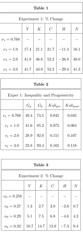
Table 1 Experiment 1: % Change Y K C H N ν1= 0.768 − − − − − ν1= 1.0 17.4 21.1 21.7 −11.4 16.1 ν1= 2.0 41.8 46.8 52.2 −26.8 40.0 ν1= 3.0 41.7 43.0 52.2 −29.4 41.3 Table 2
Exper 1: Inequality and Progressivity
Gy Gk Kakpre Kakpost
v1 = 0.768 49.4 74.5 0.045 0.045 v1 = 1.0 41.6 85.2 0.075 0.064 v1 = 2.0 28.9 92.0 0.151 0.107 v1 = 3.0 23.8 93.4 0.165 0.118 Table 3 Experiment 2: % Change Y K C H N ν0= 0.258 − − − − − ν0= 0.27 1.3 2.7 2.0 −2.6 0.7 ν0= 0.29 5.1 7.5 6.8 −4.6 4.2 ν0= 0.32 10.7 14.7 13.9 −7.3 9.4
Table 4
Exper 2: Inequality and Progressivity
Gy Gk Kakpre Kakpost
ν0= 0.258 49.4 74.5 0.045 0.045 ν0 = 0.27 48.6 78.6 0.049 0.048 ν0 = 0.29 47.8 82.8 0.054 0.052 ν0 = 0.32 46.7 86.5 0.064 0.058 Table 5 Experiment 3: % Change Y K C H N ν1 = 0.768 − − − − − v1 =∞ 203.2 265.6 254.0 10.6 184.5 Table 6
Exper 3: Inequality and Progressivity
Gy Gk Kakpre Kakpost
ν1= 0.768 49.4 74.5 0.045 0.045 v1=∞ 69.8 1.0 0.284 0.302
Figure 1 0 0.5 1 1.5 2 2.5 3 3.5 4 4.5 5 0 0.05 0.1 0.15 0.2 0.25 0.3 0.35
Personal Marginal Income Tax Function
η1 = .768 η1 = 2 η1 = 3
Table 7
Flat Tax Experiments Setup Types of Risk Effect on Aggregates Effect on Distribution
Conessa and Krueger (2006) OLG; idiosyncratic wages, death Y, K, H,N, C, r increase Giniy, Ginik increase
01
Ventura (1999) OLG idiosyncratic wages, death Y, K, N increase, Giniy, Ginik increase
Hunchanged,r decrease
Diaz-Gimenez and Pijoan-Mas (2006) OLG/dynastic idiosyncratic wages, retirement, death Y, K, H,N, C, r increase Giniy, Ginik, Ginic increase
Casta˜neda,Diaz-Gimenez, OLG/dynastic idiosyncratic wages, retirement, death Y, K, H,N, C, r increase Giniy, Ginik, Ginic increase
and R´ıos-Rull (1999)
Figure 2 0 0.5 1 1.5 2 2.5 3 3.5 4 4.5 5 0.05 0.1 0.15 0.2 0.25 0.3 0.35 0.4
Total Marginal Tax Function
η1 = .768 η1 = 2.0 η1 = 3.0
Figure 3 0.5 1 1.5 2 2.5 3 0.8 1 1.2 1.4 1.6 η1 Income 0.5 1 1.5 2 2.5 3 2 3 4 5 η 1 Wealth 0.5 1 1.5 2 2.5 3 0.5 1 1.5 η 1 Consumption
Figure 4 0.5 1 1.5 2 2.5 3 0.2 0.25 0.3 0.35 0.4 η 1 Hours 0.5 1 1.5 2 2.5 3 0.7 0.8 0.9 1 η 1 Labor Input 0.5 1 1.5 2 2.5 3 1.08 1.1 1.12 1.14 η 1 Wages
Figure 5 0 10 20 30 40 50 60 70 80 90 100 0 0.05 0.1 0.15 0.2 0.25 0.3 0.35 0.4 0.45 0.5
Hours across ε by Percentile
Figure 6 0 10 20 30 40 50 60 70 80 90 100 0 0.05 0.1 0.15 0.2 0.25 0.3 0.35 0.4 0.45 0.5
Hours across ε by Percentile
Figure 7 0 10 20 30 40 50 60 70 80 90 100 0 5 10 15 20 25 30 35 40
Effective Labor across ε by Percentile
Figure 8 0 10 20 30 40 50 60 70 80 90 100 0 5 10 15 20 25 30 35 40
Effective Labor across ε by Percentile
Figure 9 0 10 20 30 40 50 60 70 80 90 100 0 5 10 15
Income Distribution by Percentile
0 10 20 30 40 50 60 70 80 90 100 0 5 10 15 0 10 20 30 40 50 60 70 80 90 100 0 5 10 15 η1 = 2.0 η1 = 3.0 η1 = 0.768
Figure 10 0 10 20 30 40 50 60 70 80 90 100 −50 0 50 100 150
Wealth Distribution by Percentile
0 10 20 30 40 50 60 70 80 90 100 −50 0 50 100 150 0 10 20 30 40 50 60 70 80 90 100 −50 0 50 100 150 η1 = 0.768 η1 = 2.0 η1 = 3.0
Figure 11 0.5 1 1.5 2 2.5 3 0.2 0.3 0.4 0.5 0.6 0.7 0.8 0.9 1 ν1 Gini Coefficient
Figure 12 0 0.5 1 1.5 2 2.5 3 3.5 4 4.5 5 0 0.05 0.1 0.15 0.2 0.25 0.3 0.35 income
Personal Marginal Income Tax Function
η0 = .258 η
Figure 13 0 0.5 1 1.5 2 2.5 3 3.5 4 4.5 5 0 0.05 0.1 0.15 0.2 0.25 0.3 0.35
Total Marginal Tax Function
income
η0 = .258 η
Figure 14 0.26 0.27 0.28 0.29 0.3 0.31 0.32 1 1.05 1.1 1.15 Income 0.26 0.27 0.28 0.29 0.3 0.31 0.32 2.8 3 3.2 3.4 Wealth 0.26 0.27 0.28 0.29 0.3 0.31 0.32 0.75 0.8 0.85 0.9 ν0 Consumption
Figure 15 0.26 0.27 0.28 0.29 0.3 0.31 0.32 0.3 0.31 0.32 0.33 Hours 0.26 0.27 0.28 0.29 0.3 0.31 0.32 0.65 0.7 0.75 Labor Input 0.26 0.27 0.28 0.29 0.3 0.31 0.32 1.08 1.1 1.12 ν 0 Wage
Figure 16 0.26 0.27 0.28 0.29 0.3 0.31 0.32 0.45 0.5 0.55 0.6 0.65 0.7 0.75 0.8 0.85 0.9 ν0 Gini Coefficients