Studying the Solar system with the International Pulsar Timing Array

arXiv:1809.10744v1 [astro-ph.EP] 27 Sep 2018

Studying the solar system with the International Pulsar

Timing Array

R. N. Caballero,1⋆_{Y. J. Guo,}2_{K. J. Lee,}2,1_{†P. Lazarus,}1_{D. J. Champion,}1 _{G. Desvignes,}1_{M. Kramer,}1,3_{K. Plant,}4

Z. Arzoumanian,5 _{M. Bailes,}6 _{C. G. Bassa,}7 _{N. D. R. Bhat,}8 _{A. Brazier,}9,10 _{M. Burgay,}11 _{S. Burke-Spolaor,}12,13

S. J. Chamberlin,14 _{S. Chatterjee,}10,15 _{I. Cognard,}16,17 _{J. M. Cordes,}10,15 _{S. Dai,}18 _{P. Demorest,}19 _{T. Dolch,}20

R. D. Ferdman,21 _{E. Fonseca,}22 _{J. R. Gair,}23 _{N. Garver-Daniels,}12,13 _{P. Gentile,}12,13 _{M. E. Gonzalez,}24,25

E. Graikou,1 _{L. Guillemot,}16,17 _{G. Hobbs,}18 _{G. H. Janssen,}7,26 _{R. Karuppusamy,}1 _{M. J. Keith,}3 _{M. Kerr,}27

M. T. Lam,12,13 _{P. D. Lasky,}28 _{T. J. W. Lazio,}29 _{L. Levin,}12,3 _{K. Liu,}1 _{A. N. Lommen,}30 _{D. R. Lorimer,}12,13

R. S. Lynch,31_{D. R. Madison,}31_{R. N. Manchester,}18_{J. W. McKee,}3,1_{M. A. McLaughlin,}12,13_{S. T. McWilliams,}12,13

C. M. F. Mingarelli,1,32 _{D. J. Nice,}33 _{S. Os lowski,}34,1,6 _{N. T. Palliyaguru,}35 _{T. T. Pennucci,}36 _{B. B. P. Perera,}3

D. Perrodin,11 _{A. Possenti,}11 _{S. M. Ransom,}31 _{D. J. Reardon,}28,18 _{S. A. Sanidas,}37,3 _{A. Sesana,}38 _{G. Shaifullah,}7

R. M. Shannon,39,6 _{X. Siemens,}40 _{J. Simon,}29 _{R. Spiewak,}40,6 _{I. Stairs,}25 _{B. Stappers,}3 _{D. R. Stinebring,}41

K. Stovall,19 _{J. K. Swiggum,}40 _{S. R. Taylor,}42_{G. Theureau,}16,17,43 _{C. Tiburzi,}1,34 _{L. Toomey,}18 _{R. van Haasteren,}29

W. van Straten,44_{J. P. W. Verbiest,}34,1 _{J. B. Wang,}45_{X. J. Zhu,}28,39 _{and W. W. Zhu}46,1 Affiliations are listed at the end of the paper

1 October 2018

ABSTRACT

Pulsar-timing analyses are sensitive to errors in the solar-system ephemerides (SSEs) that timing models utilise to estimate the location of the solar-system barycentre, the quasi-inertial reference frame to which all recorded pulse times-of-arrival are referred. Any error in the SSE will affect all pulsars, therefore pulsar timing arrays (PTAs) are a suitable tool to search for such errors and impose independent constraints on relevant physical parameters. We employ the first data release of the International Pulsar Timing Array to constrain the masses of the planet-moons systems and to search for possible unmodelled objects (UMOs) in the solar system. We employ ten SSEs from two independent research groups, derive and compare mass constraints of planetary systems, and derive the first PTA mass constraints on asteroid-belt objects. Constraints on planetary-system masses have been improved by factors of up to 20 from the previous relevant study using the same assumptions, with the mass of the Jovian system measured at 9.5479189(3)×10−4M⊙. The mass of the dwarf planet Ceres

is measured at 4.7(4)×10−10M⊙. We also present the first sensitivity curves using real

data that place generic limits on the masses of UMOs, which can also be used as upper limits on the mass of putative exotic objects. For example, upper limits on dark-matter clumps are comparable to published limits using independent methods. While the constraints on planetary masses derived with all employed SSEs are consistent, we note and discuss differences in the associated timing residuals and UMO sensitivity curves.

Key words: pulsars: general – methods: data analysis, statistical – ephemerides

⋆

E-mail:[email protected] † E-mail:[email protected]

1 INTRODUCTION

Millisecond pulsars (MSPs) are the most stable rotators known to date in the observable Universe. Pulsar timing

(see e.g. Lorimer & Kramer 2005) is a powerful technique through which we record the times-of-arrival (TOAs) of the pulses and use a sophisticated model to convert the topocen-tric TOA, or site arrival time, to the pulse time-of-emission in the pulsar’s co-moving reference frame. The success of the model’s fit is assessed from the timing residuals—the difference between the observed and the model-predicted TOAs—which capture all the information unaccounted for in the timing model. Timing residuals from contemporary high-precision timing of the brightest and most stable MSPs observed are at levels of a few hundreds of nanoseconds (see e.g.Verbiest et al. 2016).

The high precision with which MSPs can be timed has made them the primary targets for studies of gravity in the (quasi-stationary) strong field regime, primarily through the studies of their orbital behaviour and especially when in tight orbits with other neutron stars (see e.g. Damour 2009, for a review). Additionally, MSPs can be used as refer-ence clocks to study interesting phenomena that affect their TOAs but are extrinsic to their rotational and orbital be-haviour. It is self-evident that it is to our advantage to use multiple MSPs to observe such extrinsic phenomena when possible, especially when trying to measure an effect which is expected to affect TOAs from all MSPs and depends on the pulsar’s sky position. We refer to such an ensemble of regularly observed MSPs as a pulsar timing array (PTA;

Foster & Backer 1990). The primary scientific goal of PTA researchers is the direct detection of low-frequency gravita-tional waves (GWs), at nHz frequencies, including stochastic GW backgrounds (GWBs). Three collaborations are cur-rently leading these efforts, namely the European Pulsar Timing Array (EPTA; Desvignes et al. 2016), the North-American Nanohertz Observatory for Gravitational Waves (NANOGrav; Arzoumanian et al. 2015), and the Parkes Pulsar Timing Array (PPTA; Reardon et al. 2016). These collaborations work together under the International Pulsar Timing Array consortium (IPTA;Verbiest et al. 2016) in an effort to combine data, resources and expertise to maximise their scientific output.

While the timing model includes the pulsar’s rota-tional, astrometric, and orbital parameters, and accounts for the time-delay effects of the interstellar medium on the pulsed-signal propagation, it is in fact the transformation of the observation site arrival time to the arrival time at the solar-system barycentre (SSB) that may introduce cor-related signals in the TOAs most likely to interfere with the GWB searches. Such correlated signals may arise from er-rors in the terrestrial time standards and the solar-system ephemeris (SSE) used to predict the position of the SSB at any given time of interest. The correlated signals from these two types of errors result in monopolar and dipolar spatial correlations, respectively (see Tiburzi et al. 2016), leading to cross-correlations in the timing residuals of pulsar pairs that may resemble those from a GWB, which have their basis on the quadrupole angular correlation pattern caused by GWs (Hellings & Downs 1983). The presence of signals from clock and SSE errors increases the false-alarm proba-bility of GW detection with PTAs (Tiburzi et al. 2016). In principle, these signals are distinguishable from each other if the data is sufficiently informative, and to manage this, it is especially important to increase the number of MSPs con-tributing to the analysis and to the sampling of the

cross-correlation curve (Siemens et al. 2013; Taylor et al. 2016). While we examine methods to minimise these errors and mitigate their effects when searching for GWs in the PTA data, one can also use the data to extract scientific informa-tion on topics other than GWs. In particular, PTA data have been employed to develop an independent pulsar-based time standard (Hobbs et al. 2012) and to constrain the masses of the solar-system planetary systems (SSPS) (Champion et al. 2010, henceforth CHM10).

The SSEs that we use for pulsar timing are constructed via numerical integrations of the equations of motion for the known solar-system bodies. These integrations are subject to a wealth of observational data from telescopes, radio and laser ranging and spacecrafts orbiting the planets and their moons, when available. Such input data also include esti-mates of the masses of the planets and other important solar-system bodies. Observationally, it is not the mass, M, but the gravitational parameter of the bodies that is determined, i.e. GM where G is the universal constant of gravitation. This parameter can be determined with much higher preci-sion than the gravitational constant (see e.g.Petit & Luzum 2010), a fact that limits the precision of measurements ofM

in SI units. For this reason, the masses solar-system bod-ies such as the planets are expressed as the ratios of their gravitational parameters to the solar gravitational parame-ter (heliocentric gravitational constant),GM⊙.

New data are added over time, so that newer SSEs are subject to data of better accuracy and observational sam-pling. Many of the involved parameters are fitted and ad-justed while creating the final SSE. As noted in CHM10, while this process gives accurate predictions for the posi-tions of the planetary-systems with respect to the Earth-Moon system, they do not manage to constrain the masses much better than the measurements used as initial values. This is reflected by the fact that typically the ratios of the gravitational parameters of the planetary systems with re-spect to the solar parameter are held fixed during numerical integrations. What changes between SSE versions with re-spect to the reference planetary masses is either the initial mass values of the planetary systems, for example after new mass estimates by spacecraft fly-bys, and/or the estimate of the solar gravitational parameter, which can be a fitted pa-rameter in the SSE. Therefore, the input planetary masses in principle differ between the various SSE versions. With this in mind, CHM10 search for errors in the masses of the planetary systems, as the most possible errors that pulsar-timing data could identify.

In this paper we focus on extending the work of CHM10 using the first IPTA data release (IPTA DR 1;Verbiest et al. 2016). In addition to improving the constraints on the SSPS masses, we provide the first PTA constraints on the most massive asteroid-belt objects (ABO) and employ a recently-published algorithm (Guo, Lee & Caballero 2018, henceforth GLC18) to search for possible unmodelled ob-jects (UMOs) in Keplerian orbits in the solar system. We also make a quantitative comparison of SSEs provided by two independent groups, namely the Institut de M´ecanique C´eleste et de Calcul des ´Eph´em´erides (IMCCE) and the Jet Propulsion Laboratory (JPL).

The rest of the paper is organized as follows. In Sec-tion2we briefly overview the IPTA DR 1 and list the MSPs used in the present study and their basic observational

prop-erties. In Section3we describe the analysis methods, which includes the details of single-pulsar noise analysis and analy-ses for constraining the mass of the eight planetary systems and ABOs, as well as the masses of UMOs. The results of the analyses are presented in Section4. We finally discuss scientific implications of our results and our conclusions in Section5.

2 DATA SET: THE IPTA DR 1

IPTA DR 1 is described in Verbiest et al. (2016), and we only give a brief overview in this section. The full data set consists of TOAs from 49 MSPs. Data were collected by the three regional PTAs over a total time-span of up to 27.1 yr using seven telescopes across the world, namely the Effelsberg Radio Telescope, the Lovell Telescope, the Nan¸cay Radio Telescope, and the Westerbork Synthesis Radio Telescope by the EPTA, the Arecibo Observatory and the Green Bank Telescope by NANOGrav, and the Parkes Radio Telescope by the PPTA. The IPTA DR 1 data set was constructed by combining data that were published in Kaspi, Taylor & Ryba(1994),Demorest et al.

(2013), Manchester et al. (2013), Zhu et al. (2015), and

Desvignes et al.(2016).

It is important to note that the TOAs from the dif-ferent telescopes and difdif-ferent studies were calculated with various methods. Although all TOA calculations were based on template-matching methods (Taylor 1992), where each observed profile is cross correlated with a profile template of arbitrary phase, there are technical differences regarding issues such as the methods to create the pulse-profile tem-plates, and algorithms for optimal template matching. There are also different approaches with regards to the way that the recorded information is used. For example, in some cases the total intensity profiles were used, which are created by summing the flux of all polarization modes, frequency bands and sub-integrations, while in others cases, one TOA was calculated per frequency band. These choices reflect differ-ences in the sensitivity of instruments over time and analysis methods which have developed to address them. For exam-ple, data from a receiver with limited total bandwidth would use total intensity profiles to achieve useful signal-to-noise ratio, while a more modern broadband receiver can achieve sufficient signal-to-noise ratio with sub-bands of the total bandwidth. In this case, one may opt to produce TOAs per sub-band as a way to mitigate, for example, effects of possi-ble evolution of the pulse profile over the observing frequency (see e.g.Xilouris et al. 1996;Kramer et al. 1999), or possi-ble noise that is limited in certain sub-bands (Lentati et al., 2016; Cordes, Shannon & Stinebring 2016). One may also opt to not integrate profiles over time for short-period pul-sars in order to better sample the orbit (e.g.Desvignes et al. 2016).

For MSPs for which data from more than one PTA were available, the IPTA data combination increased the time-span of the MSP data, as well as their cadence and observing-frequency coverage. Increased time-span and ca-dence allows improved sampling of orbits at longer and shorter periods, respectively. They also lead to better char-acterisation of low- and high-frequency noise properties. Noise mitigation is further aided by improved

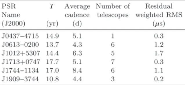
observing-Table 1. General characteristics of the IPTA DR 1.0 data (Verbiest et al. 2016) for the MSPs used in this study (note that PSR J0437−4715 was not used to derive mass limits of solar-system bodies; see Section4.1). For each pulsar we note the to-tal time-span,T, the average cadence, the number of telescopes contributing data, and the weighted root-mean-square (RMS) of the timing residuals (after subtracting the waveform of the DM variations) The residual RMS was derived using the planetary ephemeris DE421.

PSR T Average Number of Residual

Name cadence telescopes weighted RMS

(J2000) (yr) (d) (µs) J0437−4715 14.9 5.1 1 0.3 J0613−0200 13.7 4.3 6 1.2 J1012+5307 14.4 6.3 5 1.7 J1713+0747 17.7 5.1 7 0.3 J1744−1134 17.0 8.4 6 1.1 J1909−3744 10.8 4.4 3 0.2

frequency coverage which is particularly crucial in measuring chromatic noise processes related with the turbulent ionised interstellar medium. The combination of data from multiple telescopes, when available, also offers the chance to use in-dividual data sets in the same observing-frequency bands to search for noise due to systematics (Lentati et al. 2016).

The IPTA DR 1 served as a first testing ground for the use of pulsar-timing noise models that were more complex compared to previous studies such as Arzoumanian et al.

(2015), Caballero et al. (2016), or Reardon et al. (2016), which only used data from individual PTAs. It was exactly the aforementioned properties of the IPTA DR 1 that mo-tivated the inclusion of additional noise components in the noise analysis presented inLentati et al.(2016). The analy-sis was made in particular to attempt to distinguish between noise specific to each pulsar and noise due to systematics in the data of a given observing system, or noise that is associ-ated with a specific observing frequency band. The intent of introducing the latter noise term is to probe chromatic noise that does not follow the dispersive law of cold homogeneous plasma, associated with temporal dispersion measure (DM) variations (see e.g.Keith et al. 2013;Lee et al. 2014).

In the present paper we study the timing data from six MSPs in total and employed data from five of these to con-strain the masses of solar-system bodies. The MSPs were selected based on the contribution of each MSP to the over-all results as discussed in Section4.1. The key observational properties of the data for each of these pulsars are presented in Table 1. By comparison to the IPTA DR 1 data, the one change we have made is related to PSR J1713+0747. The large number of TOAs (19972) would make the current analysis significantly computationally expensive. This large number of TOAs primarily stems from NANOGrav data, which are not averaged over the observing frequency band, resulting in one TOA per frequency channel. To reduce the computational cost for PSR J1713+0747 we employed the

tempo2 _routine AverageData _{and produced an average}

TOA for each epoch per observing frequency band by sum-ming up all channels across the frequency band.

3 ANALYSIS METHODS

We have implemented two methods to study the solar system with the IPTA DR 1. Both methods rely on searching for residuals induced by the periodic oscillation of the SSB due to the presence of a mass in orbit that is not accounted for by the pulsar timing models. This mass can either be a difference from the real mass of a solar-system body to that assumed by the SSE, for which we employed the method discussed in Section3.2, or the mass of a UMO not included in the SSE, for which we employed the method discussed in Section3.3.

We clarify here, that in this study we are only mod-elling possible errors in the SSE reference masses. We do not examine the effects of positional errors. Under this model, possible small errors in orbital elements could be absorbed in the mass-error parameter. As we noted on Section1, we expect that mass errors are more likely to be detected first with pulsar timing analysis, however, sensitivity to errors in orbital elements are not excluded. The GLC18 method can also be focused on applying upper limits on orbital param-eter of UMOs, but this is beyond of the scope of this study. We discuss further work in pulsar-timing research that at-tempts to extend PTA studies to orbital elements of planets in Section5.

Prior to discussing the SSE analysis, we first give an overview of the single-pulsar timing and noise analysis.

3.1 Single-pulsar timing and noise analysis

As with other applications of PTAs, constraining the masses of known or unknown bodies in orbit around the SSB re-quires good characterisation of the noise in individual pul-sar data (see Cordes 2013; Verbiest & Shaifullah 2018, for reviews on sources of noise in pulsar timing), as noise com-ponents may have significant power at frequencies related to a planetary orbit. Insufficient accounting of the noise can lead to significant bias on the measured values of the tim-ing parameters and their uncertainties (Coles et al. 2011;

van Haasteren & Levin 2013). CHM10 pointed out these ef-fects in the context of constraining planets’ masses and specifically did not include one of the four pulsars they used, PSR J0437−4715, when estimating the mass error of Mars. Specifically, CHM10 argued that its noise model was not sufficient to account for spectral features close to the orbital frequency of Mars, and including this pulsar would thus bias the solution for the specific planet.

For the work presented in this paper, for each pulsar we created different timing and noise models for each SSE. The initial phase-coherent timing models were obtained using the timing software tempo2 _{(Hobbs, Edwards & Manchester}

2006). tempo2 uses a previously derived timing model

(which could be as simple as the pulsar discovery position and rotational frequency) and iteratively performs a least-squares fit of the model to the TOAs until the reduced chi-squared of the residuals is minimized. tempo2 applies a linearised approximation to calculate the small, linear off-sets of model parameters from the pre-fit value (see also

Edwards, Hobbs & Manchester 2006). The least-squares fit can be unweighted or weighted according to the TOA un-certainties. Throughout this work, our timing solutions use weighted fits. These initial individual pulsar-timing

mod-els do not include parameters related to errors in the SSE or any noise components. We then employed temponest

(Lentati et al. 2014) to perform a Bayesian (simultaneous) timing and noise analysis, with the same noise modelling used, for example, in Caballero et al. (2016). temponest

samples the joint parameter space of the timing and noise parameters usingMultinest_{(Feroz et al. 2009), a Bayesian}

inference algorithm based on nested sampling (seeSkilling 2004), while evaluating the timing model at each point of the parameter space using thetempo2_algorithms.

Before proceeding to the correlated-signal analysis, we produced the final noise models employing the analysis pack-age that we use to make the search for errors in the SSE in order to have a consistent mathematical noise-model parametrization. During this last stage, we performed a Bayesian noise analysis while analytically marginalising over the timing parameters, also using Multinestas the sam-pler. In brief, the noise model consists of the following com-ponents:

• Uncorrelated noise terms, modelled with a pair of cor-rections to the TOA uncertainties per observing system (white noise). The temponest _{analysis includes an EFAC}

(for Error FACtor, a multiplicative factor) and an EQUAD (for Error in QUADrature, a factor added in quadrature). The application of these terms attempts to create a timing solution where appropriate relative weights between the dif-ferent observing systems are given, since TOA uncertainties calculated via template-matching methods, do not always fully account for the TOA scatter. EFACs are used to correct underestimation of the uncertainty, for example due to low signal-to-noise ratio of the observed pulse profile, differences in the pulse profile and the template or presence of noise other than white radiometer noise in the profile, at signifi-cant levels. EQUADs are primarily used to account for addi-tional scatter in the TOAs due to physical processes such as pulse phase jitter (e.g.Liu et al. 2012;Shannon et al. 2014). The corrected TOA uncertainty,σˆ, and initial uncertainty,

σ, are then related as

ˆ

σ2=(σ·EFAC)2₊EQUAD2 (1) During the final noise analysis, we applied a ‘global’ EFAC per pulsar, to regularize the white-noise level against the other noise components.

• An achromatic (observing-frequency independent) low-frequency stochastic component (red noise) per pulsar, mod-elled as a wide-sense stationary stochastic process with a one-sided power-law spectrum of the form

S(f)= A 2 f f fc 2 ˜α , (2)

where f is the Fourier frequency, fc = 1yr−1 _{is a}

ref-erence frequency, A is the amplitude in units of time, and α˜ is the spectral index. This noise component is added to model primarily physical noise from irregulari-ties in the rotation of the pulsar, often referred to as ‘spin noise’ (e.g. Shannon & Cordes 2010; Kramer et al. 2006). In the absence of other dedicated model components (see

Lentati et al. 2016), this component will also include noise due to possible systematics in the data.

• A chromatic (observing-frequency dependent) low-frequency stochastic component (DM noise). It has the same

spectral properties as the red-noise component, but with the restriction that the induced residuals reflect TOA delays that follow the dispersive law of cold homogeneous plasma (e.g.Landau & Lifshitz 1960), i.e. the time delay of a signal at two observing frequencies,ν1andν2, along a line-of-sight

with DM value, D_l, is ∆TDl =κ Dl pc cm−3 _ν1 GHz −2 − ν2 GHz −2 , (3) where κ=4.15×10−3 s.

The power-law power spectra used to describe the stochastic noise components have sharp cut-offs at f₌1/T, withTthe data span. This cut-off reflects the fact that power at frequencies below1/T is fitted out by the timing model, as discussed in previous works (van Haasteren et al. 2009;

Lee et al. 2014). In particular, we fit for the rotational period and period derivative to remove the low-frequency power of the red noise, and the DM first and second derivatives to remove the low-frequency power of the DM-variations noise. As such, a linear and a quadratic term for DM-variations are always implemented in the (deterministic) timing mod-els used in this work.

Finally, we note that the timing model also needs to take into account the dispersive delays from the plasma of the so-lar wind (You et al. 2007). Our timing models implement the standard tempo2 _{solar-wind model (Edwards et al. 2006),}

that assumes a spherical distribution of free electrons with a nominal density of 4 cm−3 at 1 AU. Deviations of the elec-tron density distribution from this value (e.g. due to so-lar activity or deviations from the assumed electron density distribution and/or density at 1 AU) will induce additional delay signals that become significant when the line-of-sight to the pulsar is close the to the solar disc. The result is then induced residuals with annual signatures, which peak at epochs where the pulsar is at its smallest elongation. Pul-sars with low ecliptic latitudes are more susceptible to such effects (only PSR J1744−1134 falls into that category from the pulsars used in this study). Unmitigated solar-wind sig-nals have complex power spectra and show spatial corre-lations similar to that caused by SSE errors (Tiburzi et al. 2016) so that they could interfere with the sensitivity of PTA data at high frequencies. More careful modelling of the solar wind is planned for future work. Data from new observing campaigns at lower frequencies (see e.g.Tiburzi & Verbiest 2018) can provide valuable input for better modelling and mitigation of dispersive delays from the solar wind.

3.2 Analysis method for known solar-system bodies

We first discuss our approach in searching for coherent wave-forms in the MSPs from possible errors in the SSPS masses assumed in the SSE. We employ a frequentist analysis using a code that implements the method described in CHM10.

The method considers small errors,δm, in SSPS masses,

m, so thatδm≪m. Such errors will induce residuals due to periodic linear shifts in the SSB position with the period of the planetary orbit. In such a small mass-error case, we can neglect higher-order effects on the residuals due to the SSB motion. CHM10 examined the extent of secondary ef-fects using a modified version of the DE421 SSE where the

mass of Jupiter deviated the real value by 7×10−11M⊙ (an

amount compatible to the precision that current PTAs can probe the Jovian system mass, as one can see from the re-sults in the next Section) and concluded that such effects were negligible in the case of Jupiter after fitting for the tim-ing model. We further investigated these secondary effects with methods similar to the work in CHM10 and reached similar conclusions. The cases of the inner planets, Mercury and Venus, show additional complexity because of the ef-fects on the orbit of the Earth-Moon system that errors in these planetary masses would cause. The induced residuals from such effects, however, fall into different frequencies to the orbital frequencies of the inner planets. Consequently, although a fully dynamical model could make use of such signals as additional information in constraining the plane-tary masses, we have verified that these signals, if present in the data, do not affect the results and conclusions from the narrow-frequency signal search employed in this work.

In the first-order CHM10 approximation, the induced residuals from the erroneous mass are then only associated with the (solar-system related) Rømer delay, the geometric vacuum delay of the TOA at the observatory and at the SSB. The induced residuals will reflect the shift in the position of the SSB along the barycentric position vector of the SSPS,

b, associated with an error in the pulse time-of-emission. For the multi-pulsar and multi-SSPS case, this error is calculated for each time epoch as

τ_bn,k ≈ 1 cMT n,k Õ i,j δmi(bi·Rˆj), (4)

where indices i and j refer to the i-th (out ofn) SSPS and the j-th (out of k) pulsar, respectively,bis the barycentric position vector of the SSPS,Rˆ_{j is the unit barycentric}

po-sition vector of the pulsar (or pulsar binary) barycentre,c

is the speed of light and MT is the total mass of the solar

system, which was approximated byMT≈M⊙.

Since Eq. (4) is linear,τb can be directly added to the

linear timing model of tempo2. Although a single pulsar can provide measurements of the δm parameters, Eq. (4) shows how the measurement precision is dependent on the pulsar’s sky position and, therefore, better and less biased measurements can be made by fitting for these parameters simultaneously with many pulsars. In CHM10, this was per-formed usingtempo2_{, which was appropriately modified to}

allow the δm parameters to be fitted in a ‘global’ timing analysis. Such an analysis is a simultaneous fit of the timing models of various pulsars, where a subset of the parameters, which we call global, are common for all pulsars. In this example, theδmparameters are the global parameters.

The covariance matrix for each pulsar,C, is constructed using the maximum-likelihood values of the posterior distri-bution of the Bayesian noise analysis. It is defined as

C₌C_w+C_r+C_{d, (5)}

where the constituent matrices are the white-, red- and DM-noise covariance matrices.C_wis a diagonal matrix with the main diagonal populated with the variances of the TOAs (after application of EFACs and EQUADs). The red- and DM-noise covariance matrices are populated by elements

de-fined, respectively, as (Lee et al. 2014) C_{r,i j =} ∫ ∞ 1/T Sr(f)cos(2πf ti j)df,and (6) C_{dm,i j=} κ2∫₁∞_/TSd(f)cos(2πf ti j)df ν_i2ν2_j . (7)

In the above equations, theiandjindices refer to observing epochs, andνdenotes the observing frequency.

We can now proceed to search for coherent waveforms as predicted by Eq. (4) via a global timing analysis. Dur-ing our analysis, apart from the global parameters, for each pulsar we only fitted for a limited number of timing param-eters to ensure that the condition numbers of the design matrices (discussed below) were small and matrix inversions are computationally stable. The timing parameters fitted for are the rotational frequency and its derivative, the DM and derivatives (first and second included in timing models), the pulsar position and parallax. The rotational frequency, DM, and their derivatives correlate with low-frequency noise pa-rameters andδmparameters related to the planets with the longest periods. Pulsar position and parallax are also signif-icantly affected by changes to the SSEs (see also Fig. 1 in

Caballero 2018). We have done so after confirming that the timing models were not influenced by this practice.

Using standard linear-algebra methods we fitted the timing parameters denoted with the column matrix, ǫ, as

ǫ=(AT_rAr)−1ATrA

T

qC−

1

2t, (8)

and the corresponding variances are given by

σǫ2=diag(J−1), J=D

T_C−1_{D (9)}

In these equations, t is the column matrix of the timing residuals, D_{is the design matrix (calculated with} tempo2

during the individual pulsar timing analysis),Cis the covari-ance matrix andJ_{is the Fisher-information matrix.Aqand}

Arthe Q and R decompositions of matrixA=C−

1

2D, respec-tively. The T,−1 and −12 superscripts denote the transpose,

inverse and inverse of the square root of a given matrix, re-spectively. All matrices are the total matrices, for all pulsars;

t is formed by appending all pulsar timing residuals, C is the block-diagonal matrix of all pulsar covariance matrices, and D_{is formed by appending the SSPS-waveform column}

matrices to the block-diagonal matrix of all pulsar design matrices. In this way, the SSPS-waveforms act as global pa-rameters to the fit.

The columns with the global SSPSδm waveforms are calculated using Eq. (4). The position of the pulsar is known from the timing model. The position vector of the SSPS for a given observing epoch is calculated based on the information for the SSPS orbits provided by the used SSE. IMCCE and JPL provide libraries that contain modules and functions that read in the data from the ephemerides and calculate the positions and velocities of the SSPSs for given times. IMCCE and JPL provide thecalceph1 (Gastineau et al. 2015) and

1 _{http://www.imcce.fr/fr/presentation/equipes/ASD/inpop/calceph/}

spice2_{libraries respectively. Having confirmed that both}

li-braries give completely consistent results, we used the cal-ceph_{in all related work, except the calculations regarding}

mass errors of ABOs, as discussed in Section4.2.1.

3.3 Analysis method for unknown solar-system bodies

The approximation used in CHM10 can also be employed in the case where instead of errors in the SSE’s reference mass of the SSPS, we consider the mass of UMOs, for which we then also need to model the dynamics of their motion. Such an analysis is beneficial for different reasons. Firstly, it gives the potential to PTAs to probe the masses and dynamics of any object in orbit around the SSB and to impose constraints on physical parameters of proposed or hypothetical objects (see Section4.3), such as Planet Nine (Brown & Batygin 2016) or dark matter in the solar system with specified mass distributions (Loeb & Zaldarriaga 2005;

Pitjev & Pitjeva 2013;Pitjeva & Pitjev 2013). In this study we focus on a simple model which assumes small bodies in Keplerian orbits around the SSB in order to probe to first order the sensitivity of the real PTA data set to orbiting masses in the solar system. While not specifically applied in order to constraint the parameter space of specific pro-posed objects, the analysis assumes orbits that approximate those of most solar-system bodies (excluding perturbations) and the results can serve as a confirmation of our mass con-straints on known bodies and as a means to compare the different SSEs at first order.

For this analysis, we implement the algorithm presented in GLC18, which searches for coherent waveforms from bod-ies in Keplerian orbits around the SSB, in the TOAs of all pulsars. The details of the approach to search for UMOs, including the mathematical framework, the choice of prior distributions and the analysis algorithm, can be found in GLC18. The algorithm solves the dynamical problem of bod-ies in Keplerian orbits. By neglecting higher-order effects due to the SSB motion as in CHM10 and any perturbations on the UMO from any object except the Sun, the algorithm is currently restricted to searches of small objects and that are not in orbit around a major planet. The dynamical model contains seven unknown parameters, i.e. the mass of the UMO,m, and the six Keplerian orbital parameters, i.e. the semi-major axis,a, the eccentricity,e, the longitude of the ascending node,Ω, the inclination of the orbit,i, the argu-ment of perihelion, ω, and the reference phase, φ0. For a

set of values for these parameters, the model determines the barycentric position vector of the UMO,b, and uses Eq. (4) to calculate the induced signal in the TOAsS(ξ), where we useξto denote the seven unknown parameters.

The UMO-induced waveform is now an unknown wave-form in the data, and no longer part of the timing pa-rameters. The analysis now uses the reduced likelihood (van Haasteren et al. 2009), which is used when solving the problem while analytically marginalising over the parame-ters that are not of interest (often referred to as nuisance parameters). In this case, these are all the timing param-eters, ǫ. For the multi-pulsar case, where we search for a

coherent waveform S in all pulsars, the reduced likelihood function can be written as

Λ∝p 1 |CC′| × exp©­ « −1 2 Õ i,j,I,J

(t_I,i−S(ξ)_I,i)TC′I,J,i,j(tJ,j−S(ξ)J,jª®

¬ ,

(10) where the I,J indices denote pairs of pulsars, the i,j

indices denote pairs of time epochs, and C′ ₌ C−1 − C−1D(DTC−1D)−1DTC−1_{. We note that one can use the}

alternative formulation of the likelihood introduced in

Lentati et al.(2013). By applying Bayes’s theorem, one can proceed to perform Bayesian parameter estimation as

P(ζ|X) ∝P(ζ)_Λ. (11)

In this compact notation, X is the data and ζ are all the model parameter we want to sample, that is, the Keplerian orbital parameters of the UMO and the pulsar-noise param-eters we opt to fit simultaneously. Therefore, P(ζ|X) is the posterior probability distribution of the parameter(s) of in-terest, and P(ζ) is the prior probability distribution of the parameter(s). The parameter space is explored using Multi-nest.

The analysis algorithm for UMOs offers flexibility in the analysis, allowing analytical marginalization over the timing parameters and limiting the prior range of orbital parame-ters or fixing them to a given value. For the work presented in this paper, we analytically marginalize over the timing pa-rameters and simultaneously search over the UMO orbital parameters and pulsar-noise parameters.

Following the same procedure as in GLC18, we first ran an analysis using the least informative priors for the parameters in order to get the posterior distributions from which we can determine whether we have a possible detec-tion of a UMO. These priors are uniform in the log-space for the parameters with dimension and uniform for dimension-less parameters. In the non-detection case, as is the case in all our IPTA DR 1 analyses, we proceeded to a follow-up, upper-limit analysis to determine the data’s sensitivity to any given UMO mass at any semi-major axis value. For the upper-limit analysis, we changed the mass priors to uniform in linear space and performed Bayesian inference for a grid of fixed semi-major axis values. We will refer to these upper limits of the mass as a function of the semi-major axis as the mass sensitivity curves.

4 ANALYSES AND RESULTS

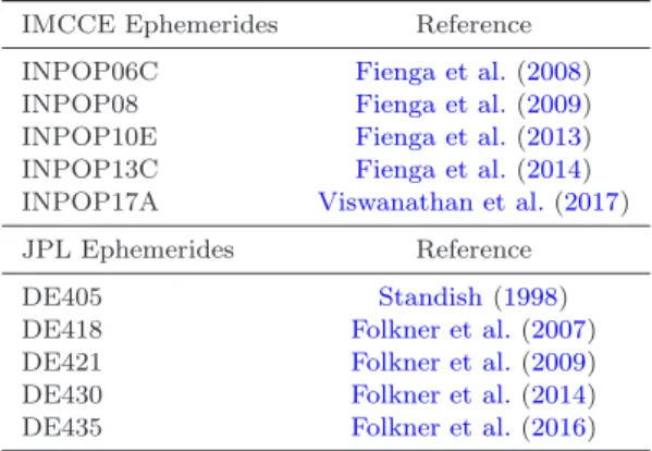
The analysis with our implementation of the CHM10 method used ten different SSEs, five from IMCCE (desig-nation “INPOP”) and five from JPL (desig(desig-nation “DE”). An overview of the SSEs we employed can be found in Table2. Before proceeding to searches for correlated SSE-error sig-nals across pulsars, we performed some preliminary searches for errors in masses of SSPSs using single-pulsar data to check the effects of the noise model we select and to com-pare the performance of our implementations of the CHM10 method with that of tempo2_{. We also made a first-order}

Table 2.List of SSEs used in the analyses. IMCCE Ephemerides Reference INPOP06C Fienga et al.(2008) INPOP08 Fienga et al.(2009) INPOP10E Fienga et al.(2013) INPOP13C Fienga et al.(2014) INPOP17A Viswanathan et al.(2017)

JPL Ephemerides Reference

DE405 Standish(1998)

DE418 Folkner et al.(2007)

DE421 Folkner et al.(2009)

DE430 Folkner et al.(2014)

DE435 Folkner et al.(2016)

comparison of the effects on pulsar timing from choosing a different SSE during the analysis.

We tested whether using the noise model described in Section 3.1 produced significantly different results than when using the more complex models published in

Lentati et al.(2016). In that work, the SSE DE421 was used, so we used this SSE for a proper comparison. We used single-pulsar constraints onδmof the SSPSs usingtempo2_{, which}

can use both types of noise models for single-pulsar cases to constrain the mass error. This test was useful for investi-gating whether any of the pulsars had such noise properties that using a simpler noise model would create a significant bias in the multi-pulsar, correlated search for errors in the SSE input masses of solar-system bodies. We did not find any statistically significant differences between theδm mea-surements using the different noise models. We then pro-ceeded to compare the single-pulsar results usingtempo2

and the algorithm described here, implementing the noise model used in this work. We found theδmmeasurements to be consistent using the two different codes.

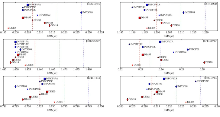
We carried out a first-order examination of the effects of our choice of SSE during the timing analysis. As the tim-ing residuals are the primary metric of the completeness of the timing model, we compared the residuals’ weighted root-mean-square (RMS) for each pulsar when using differ-ent SSEs. The results for six MSPs (see next section for the selection of pulsars) are summarized in Fig. 1. If we assume that the residual RMS will be minimal for the best-performing SSE, the SSE ranking varies for different pulsars, suggesting that the SSE performance is dependent on the sky position. It is known that the differences between the pairs of SSEs have various sky patterns, an effect that can be illustrated using simulated data (seeCaballero 2018).

It is important to keep in mind that SSE re-lated residuals can be fitted out by a number of tim-ing parameters if they have power at those frequencies (Blandford, Narayan & Romani 1984). We are aware that this happens with parameters such as the annual term of the position of the pulsar and other astrometric parameters (see e.g. Madison, Chatterjee & Cordes 2013; Wang et al., 2017). Residual signals due to possible SSE imperfections may also be covariant with pulsar noise parameters. As a result, in the absence of independent constraints on pulsar timing parameters, the SSE ranking based on the timing residuals RMS does not necessarily mean overall better ac-curacy on the data used to construct the SSE.Madison et al.

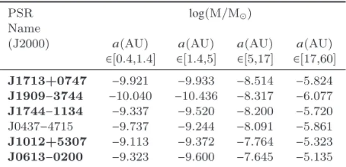
Table 3.Average sensitivity to mass of UMOs in Keplerian orbits in four ranges of the semi-major axis, a, for single-pulsar cases. The table reports the sensitivity as the logarithms of the average of the 1σ upper limits on the mass of UMOs within each semi-major axis range. The MSPs are listed in order of sensitivity (best to worse) in the intervala∈[5,17]. Given the data set’s cadence and time-span, this is the interval where the analysis performance is expected to impact mostly on our results. MSPs in boldface were selected to derive the mass constraints of SSPS, ABOs and UMOs (see discussion in main text).

PSR log(M/M⊙)

Name

(J2000) a(AU) a(AU) a(AU) a(AU)

∈[0.4,1.4] ∈[1.4,5] ∈[5,17] ∈[17,60] J1713+0747 −9.921 −9.933 −8.514 −5.824 J1909−3744 −10.040 −10.436 −8.317 −6.077 J1744−1134 −9.337 −9.520 −8.200 −5.720 J0437−4715 −9.737 −9.244 −8.091 −5.861 J1012+5307 −9.113 −9.372 −7.764 −5.323 J0613−0200 −9.323 −9.600 −7.645 −5.135

(2013) also demonstrated that the ability of the noise models included in the timing analysis to prevent leakage of residu-als in astrometric parameters depends on the total timespan of the pulsar data set. Therefore, a given SSE may perform differently in terms of the residual RMS for pulsars with dif-ferent time-spans, even when their true noise properties are similar, since de-correlating pulsar noise, SSE residuals and astrometric parameters requires sufficient data length. Ad-ditionally, a given SSE may be over- or under-performing by comparison to another SSE for different solar-system bodies when used in pulsar timing, so the data-span can further influence the overall performance of an SSE.

While at present the differences in the RMS values of the residuals using different SSEs are within the noise-fluctuation levels, it is clear that without a full account of such effects in the timing model, cross-checking our results using various SSEs makes studies such as the one presented in this paper more meticulous and robust. A direct conse-quence of the issues discussed above is that a result regarding the constraints on planetary masses becomes more reliable when using pulsars at as many sky positions as possible and with comparable timing precision and overall data quality, when possible.

4.1 Selection of pulsars for analysis

The last point to consider before proceeding to the anal-ysis is which pulsars to use. Searching correlated signals with many pulsars is a computationally intensive task. It has thus been common practice to attempt a ranking of the pulsars available, in order to choose those expected to con-tribute the most to the analysis. The type of signal sought, the noise characteristics of each pulsar as well as the details of each pulsar’s data quality (cadence, time-span, observing frequencies, etc) play crucial roles in the ranking.

We made a single ranking of the pulsars that we used for both analysis methods described in Section3so that we are able to directly compare the results of the analysis for mod-elled and unmodmod-elled solar-system objects. Our approach was to use the GLC18 Bayesian code described in Section3.3

to determine the sensitivity curves of the single-pulsar data to UMO masses. For this, we used the SSE DE421. Table3

shows a breakdown of the average sensitivity in four inter-vals of semi-major axis, chosen to be equal in logarithmic space. One can see that the relative sensitivity between pul-sars can change over the semi-major axis or equivalently over the period of the Keplerian orbit. Given that the time-spans of our pulsar data sets are between the orbital periods of Jupiter and Saturn while the cadence for all pulsars is much shorter than the period of Mercury, we anticipate that the sensitivity of the pulsars in the third semi-major axis in-terval (5< a/AU<17) is the most impactful to our results. We therefore made a priority list according to the average sensitivity in that interval. Beyond the top six pulsars, the average sensitivity drops significantly and we therefore de-cided not to use more MSPs for this work.

The set we used to derive mass limits eventually con-sisted of five pulsars (highlighted in Table 3). Despite the fact that PSR J0437−4715 is fourth in the ranking, we de-cided to not include it in this analysis. This is because ex-amination of the posterior distribution of the orbital pa-rameters from the single-pulsar Bayesian analysis for UMOs using PSR J0437−4715 revealed possible systematics in the high-frequency regime (i.e. for small values of the semi-major axis) which resulted in the calculated sensitivity curve vi-olating the analytic sensitivity curve (see GLC18 for de-tails on the analytic sensitivity curve). Our analysis revealed systematics in the range of 1<a/AU<5 which complicated the upper limit analysis, and worsen the UMO mass up-per limits when including this pulsar in the multi-pulsar analysis, in contrast to the expectation from the pulsar’s noise properties and analytical sensitivity curve. To avoid the potential effects and complications due to these sys-tematics, which we reproduced using multiple SSEs, we did not include PSR J0437−4715 in constraining masses of solar-system bodies. This pulsar is very bright and as such has very small TOA uncertainties, but it is known to suf-fer from multiple sources of time-correlated noise (see e.g.

Lentati et al. 2016), which gave significant effects on our analysis exactly because of the low TOA uncertainties. We remind the reader that, as discussed in Section3.1, CHM10 assumed their noise model for PSR J0437−4715 was not pre-cise enough around the orbit of Mars (∼ 1.5AU). We will focus on the results without PSR J0437−4715, to directly compare the results of the analysis for modelled and un-modelled solar-system objects. Examining the exact origins of the systematics is beyond the scope of this paper and is left for future work.

4.2 Constraints on masses of known solar-system bodies

We used our implementation of the CHM10 method, as de-scribed in Section3.2on the five-pulsar subset of IPTA DR 1, using the ten SSEs noted in Table 2. As explained in Section3.2, our analysis seeks possible errors in the input masses, assuming that the mass error is small such that only geometric delays of the pulse propagation due to errors in the estimated position of the SSB are significantly affecting the timing residuals. The SSE input values were taken di-rectly from the header information of the SSEs using the

0.195 0.200 0.205 0.210 0.215 0.220 0.225 0.230 0.235 RMS(µs₎ DE405 DE418 DE421 DE430 DE435 INPOP06C INPOP08 INPOP10E INPOP13C INPOP17A J0437-4715 1.185 1.190 1.195 1.200 1.205 1.210 1.215 1.220 RMS(µs₎ DE405 DE418 DE421 DE430 DE435 INPOP06C INPOP08 INPOP10E INPOP13C INPOP17A J0613-0200 1.445 1.450 1.455 1.460 1.465 1.470 1.475 1.480 RMS(µs₎ DE405 DE418 DE421DE430 DE435 INPOP06CINPOP08 INPOP10E INPOP13C INPOP17A J1012+5307 0.22 0.24 0.26 0.28 0.30 RMS(µs₎ DE405 DE418 DE421 DE430 DE435 INPOP06C INPOP08 INPOP10E INPOP13C INPOP17A J1713+0747 0.710 0.715 0.720 0.725 0.730 0.735 0.740 0.745 0.750 RMS(µs₎ DE405 DE418 DE421 DE430 DE435 INPOP06C INPOP08 INPOP10E INPOP13C INPOP17A J1744-1134 0.200 0.205 0.210 0.215 0.220 0.225 0.230 0.235 0.240 RMS(µs₎ DE405 DE418 DE421 DE430 DE435 INPOP06C INPOP08 INPOP10E INPOP13C INPOP17A J1909-3744

Figure 1.The RMS of the timing residuals of the six MSPs listed in Table1, using the ten SSEs listed in Table2. The dashed red, dotted green and dashed-dotted blue lines represent RMS values which are 10, 20, and 30 ns larger than the smallest RMS achieved for the MSP in question. Note that PSR J0437−4715 was not included when calculating mass constraints for solar-system bodies (see Section4.1).

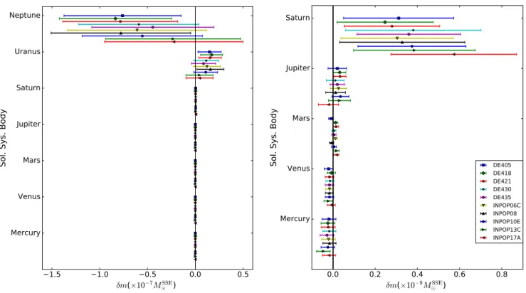
Fig.2shows the results of the analysis for all ten SSEs. The analysis included all planetary systems (excluding the Earth-Moon system). For planets with moons we refer to the position and mass of the system’s barycentre. The results from the various SSEs are statistically consistent. We also observe that despite the fact that mostδmmeasurements are consistent with zero near the 1σ level, for each planet the central values from the various SSEs are not randomly dis-tributed around zero but have consistent, systematic biases, i.e. are either positive or negative. The only exceptions are INPOP17A for Jupiter, and INPOP08 and DE405 for Mars, although this can be compensated by the very small values with respect to the uncertainties. The most likely reason for these systematic bisases is that at this given level of timing precision the results are almost completely constrained by the data, rather that from differences between SSEs within the limits of the random noise from the measurements they use as input data.

Fig. 3shows the distribution of the significance (cen-tral value divided over the 1σuncertainty) of the measure-ments. We see that 38.57 per cent of the cases (27 out of 70) show a measurement with a significance above 1σ. This distribution of errors is very close to a Gaussian distribu-tion(where the corresponding percentage would be at most 31.73). The small difference from the expected error distribu-tion can be due to correladistribu-tions of long-orbitalδmsignals and low-frequency noise, together with the fact that the analysis assumes symmetric uncertainties. That is because when a

δmsignal correlates with noise parameters, its probability distribution may in fact be asymmetric and the uncertainty would be larger on one side of the median value than the other. Full Monte-Carlo sampling of the SSE and noise pa-rameters could be implemented in future work to have a better understanding of these correlations.

Results on Saturn and the ice giants are largely incon-clusive. The orbital periods of Uranus and Neptune (84 and 165 years, respectively) are more than six times longer than the data time-span, while their masses are more than five time smaller than the mass of Saturn. It is therefore ex-pected, a priori, that our data set will be completely in-sensitive to any possible small errors in their masses. We include them nevertheless in our analysis, since the uncer-tainties ofδmfor these planets are a good indication of the goodness of the uncertainties calculated in the presence of time-correlated noise in the pulsar data and the sufficiency of the pulsar noise models we use. In the presence of low-frequency noise, if the models underestimate the noise levels, one would expect to see significant detections ofδmfor plan-ets with periods longer than the data set’s time-span. The results are as expected, with the uncertainties onδmof the ice giants being orders of magnitude larger than the rest of the planets.

Using the results of the analysis, we derived the mass constraints of the planetary systems in the solar system using the IPTA DR 1 and the ten SSEs employed in this study. The results are summarized in Table4. Since the

so-−1.5 −1.0 −0.5 0.0 0.5

δm

M

δm

M

Figure 2.The derived central values and 1σuncertainties for errors on the masses of the planetary systems with respect to each SSE’s input values, for analyses using the ten SSEs listed in Table 2. The figure on the left-hand-side includes the ice giants to emphasize the much larger uncertainties on their derived masses. The figure on the right-hand-side excludes the ice giants for clarity. TheSSE superscript is used to denote that each result is tied to the values of the Sun’s gravitational mass of the given SSE (see main text, Section4.2for details).

0.2 0.4 0.6 0.8 1.0 1.2 1.4 1.6 1.8 2.0 Significance 0.0 0.2 0.4 0.6 0.8 1.0 1.2 N 38.57%

Figure 3.The normalised histogram of the distribution of the significance (central value divided over the 1σuncertainty) of the SSPS mass measurements. 38.57 per cent of the cases show a sig-nificance over unity, compared to the 31.73 per cent expected for a Gaussian distribution. The vertical, black, dashed line indicates the significance of 1. The red, solid line shows the corresponding cumulative distribution.

lar gravitational parameter is a fitted quantity in the SSEs, and is therefore different in each case, we express all re-sults as ratios of the planetary gravitational parameters as derived using a specific SSE (superscript SSE) with

re-spect to the nominal solar gravitational parameter,GMN_{⊙ =} 1.3271244×1020m3_s−2_{, in compliance with the guidelines}

from the 2015 IAU Resolution B33 (Mamajek et al. 2015). We follow this approach in all mass constraints results we present. While at the precision of the current data set this does not cause any differences in the results within the un-certainties, we nevertheless adopt this approach to allow cor-rect comparisons with future results. A first observation is the consistency in the uncertainties, despite fluctuations in the central values ofδm. The IPTA DR 1 data set is sensitive to mass differences of a few times10−11M⊙ for systems up

to the Jovian, which constitutes a significant improvement from the approximately10−10M⊙ reported in CHM10. We

note that for the Saturnian system, this sensitivity is approx-imately 3×10−10M⊙ while for the ice giants, the sensitivity

drops significantly to approximately10−8M⊙.

To evaluate our results, we compare them with the re-sults from CHM10 and with the current best estimates4

(CBEs) adopted by the International Astronomical Union (IAU) for the planet-moons systems. The CBEs, denoted with the CBE superscript, are selected from the literature and are derived directly from spacecraft data. For the com-parison, we also expressed the CBE results with respect to the nominal solar gravitational parameter. We note again,

3 _{Available at:}

https://www.iau.org/static/resolutions/IAU2015 English.pdf

4 _{Up-to-date information at:}

that such an approach does not change our results within the uncertainties due to the current data precision, but we follow this practice to allow better comparisons with future results and follow the recommended best practices by the IAU. Compared to CHM10, the mass constraints have im-proved by factors of 5.7, 8.5, 20, 6.7 and 4 for the planetary systems of Mercury, Venus, Mars, Jupiter and Saturn, re-spectively. In Table5, we also compare our results with the IAU CBEs. The precision of the mass constraints derived in this study for planetary systems is lower by factors that range from of∼ 3for the case of Jupiter, up to∼ 103 for Mercury. In the case of Mercury, the large difference reflects the very significant improvement in the planet’s gravity field measurements by the MESSENGER spacecraft. The CBEs for Mercury’s gravitational mass (Mazarico et al. 2014) are about a factor 103 more precise than the previous CBEs (Anderson et al. 1987).

4.2.1 Asteroid-belt objects

The main asteroid belt hosts small bodies with masses that reach up to order 10−10M⊙. With the IPTA DR 1 having

sensitivity to mass errors of the order10−11M⊙−10−10M⊙

between the orbits of Mars and Jupiter (see also next sec-tion), it is logical to attempt constraining the masses of the largest bodies of the main belt. This is the first time that PTA data are used to derive mass constraints on ABOs. As our data are only beginning to be sensitive to ABO masses, in this work we perform a pilot study and use only one SSE. Future work with more sensitive data can focus more on comparisons between the pulsar-timing constraints on ABO mass using different SSEs. We employed the SSE DE435 to-gether with additional, high-precision positional data for the ABOs from theNew Horizons SPICE Data Archive5, which were used for the New Horizons spacecraft mission. These auxiliary data are provided by JPL in thespicekernel for-mat and for this reason, for this application we use thespice

library and tools.

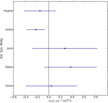
Theδmmeasurements are shown in Fig.4and Table6

presents the mass constraints derived. We produced IPTA mass constraints on the three ABOs included in the IAU body constants, namely the dwarf planet Ceres and the as-teroids Pallas and Vesta and additionally for another two large asteroids, Juno and Hygiea. For both Ceres and Pal-las, the IPTA mass constraint is only slightly over an or-der of magnitude larger than the IAU CBEs. On the other hand, the IPTA precision on the mass of Vesta is five orders of magnitude worse. This is because of a very precise new determination of the asteroid’s mass, orbital and orienta-tion parameters byKonopliv et al.(2014), which increased the precision of the mass measurement by a factor 105 _from

the previous best estimate. This was achieved by measure-ments made with radiometric tracking and optical data from the Dawn spacecraft (Russell & Raymond 2011). The Dawn space mission was specifically designed to send the space-craft in orbit around Ceres and Vesta for detailed studies. We note that although not yet adopted by the IAU, a pub-lication has recently appeared presenting results for Ceres by the Dawn mission, which has also improved the precision

5 _{https://ssd.jpl.nasa.gov/x/spk.html} −0.6 −0.4 −0.2 0.0 0.2 0.4 0.6 0.8 δm(×10−10MSSE ⊙ ) Ceres Pallas Juno Vesta Hygiea So l. Sy s. Bo dy

Figure 4.The derived central values and 1σ uncertainties for errors on the masses of five massive asteroid-belt objects with respect to the SSE’s input values, for an analysis using the DE435 SSE and updated high-precision positional data from the New Horizons SPICE Data Archive. TheSSE

superscript is used to denote that each result is tied to the values of the Sun’s grav-itational mass of the given SSE (see main text, Section 4.2for details).

of its mass measurement by a factor of 100 (Konopliv et al. 2018). For the asteroids Juno and Hygiea the uncertainty is equal or higher than the mass constraint and therefore we can only assume upper limits of 9×10−11M⊙and 6×10−11M⊙

on their masses, respectively, at the 68 per cent confidence level.

4.3 Constraints on masses of UMOs

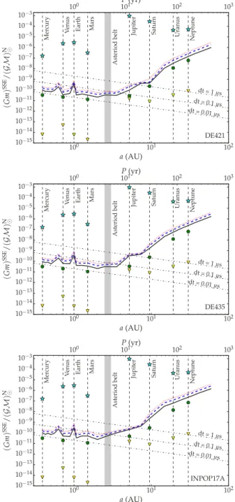
We used the same five-pulsar list as in the analysis for the SSPSs and ABOs in the previous section and employed the method outlined in Section3.3to conduct the Bayesian anal-ysis to search for UMOs. This is the first time that such an analysis has been conducted using real PTA data. Given the very high consistency in the results produced using the ten SSEs in the previous section, we opted to focus on three SSEs, namely DE421, DE435 and INPOP17A. The first was chosen for comparison reasons, since it is the SSE used in CHM10 and the IPTA DR 1 data release and noise-analysis papers (Verbiest et al. 2016;Lentati et al. 2016), while the other two were chosen because they are the latest from each SSE family among those used in this study. Table7gives an overview of the types of prior probability distributions used for the sampled parameters, as well as the ranges of their values.

We performed a blind orbital analysis, i.e. we fully searched over the UMO mass and orbital parameters. Our analysis was restricted to circular and eccentric orbits. For all three SSE cases we derived a non-detection result, and produced the mass sensitivity curves, which we present in

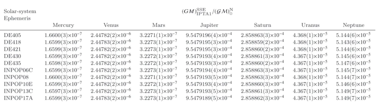
Table 4.The mass constraints on the planetary systems derived with the IPTA DR 1, using ten different SSEs, expressed as ratios of their gravitational masses to that of the nominal solar gravitational mass. (see main text, Section4.2for details). Numbers in brackets indicate the uncertainty in the last digit quoted. All results are consistent at the 1σlevel.

Solar-system (G M)SSE

IPTA1/(G M) N ⊙ Ephemeris

Mercury Venus Mars Jupiter Saturn Uranus Neptune

DE405 1.6600(3)×10−7 _{2.44782(2)×10}−6 _{3.2271(1)×10}−7 _{9.5479196(4)×10}−4 _{2.858863(3)×10}−4 _4.368(1)×10−5 _5.144(6)×10−5 DE418 1.6599(3)×10−7 _{2.44783(2)×10}−6 _{3.2273(1)×10}−7 _{9.5479195(3)×10}−4 _{2.858859(2)×10}−4 _4.368(1)×10−5 _5.143(6)×10−5 DE421 1.6599(3)×10−7 _{2.44782(2)×10}−6 _{3.2273(1)×10}−7 _{9.5479195(3)×10}−4 _{2.858860(2)×10}−4 _4.368(1)×10−5 _5.144(6)×10−5 DE430 1.6599(3)×10−7 _{2.44782(2)×10}−6 _{3.2272(1)×10}−7 _{9.5479193(4)×10}−4 _{2.858861(3)×10}−4 _4.367(1)×10−5 _5.145(6)×10−5 DE435 1.6598(3)×10−7 _{2.44782(2)×10}−6 _{3.2272(1)×10}−7 _{9.5479193(3)×10}−4 _{2.858860(2)×10}−4 _4.367(1)×10−5 _5.147(6)×10−5 INPOP06C 1.6599(3)×10−7 _{2.44782(2)×10}−6 _{3.2273(1)×10}−7 _{9.5479194(4)×10}−4 _{2.858863(3)×10}−4 _4.367(1)×10−5 _5.145(7)×10−5 INPOP08 1.6600(3)×10−7 _{2.44782(2)×10}−6 _{3.2271(1)×10}−7 _{9.5479193(5)×10}−4 _{2.858863(3)×10}−4 _4.368(1)×10−5 _5.144(7)×10−5 INPOP10E 1.6599(3)×10−7 _{2.44782(2)×10}−6 _{3.2272(1)×10}−7 _{9.5479193(4)×10}−4 _{2.858860(3)×10}−4 _4.367(1)×10−5 _5.146(6)×10−5 INPOP13C 1.6597(3)×10−7 _{2.44782(2)×10}−6 _{3.2273(1)×10}−7 _{9.5479193(5)×10}−4 _{2.858861(3)×10}−4 _4.367(1)×10−5 _5.149(7)×10−5 INPOP17A 1.6599(3)×10−7 _{2.44783(2)×10}−6 _{3.2273(1)×10}−7 _{9.5479189(5)×10}−4 _{2.858862(3)×10}−4 _4.367(1)×10−5 _5.149(7)×10−5

Table 5.Comparison between the mass constraints on the plan-etary systems from this work (IPTA1), the CHM10 results and the CBEs adopted by the IAU. Numbers in brackets indicate the uncertainty in the last digit quoted. the different results are ex-pressed in terms of the nominal solar gravitational mass (see main text, Section4.2for details). The sensitivity of the methods can be compared via the ratio of their uncertainties (σ). For IPTA values, we used the case with the highest uncertainty for each planetary system. Where multiple SSE cases gave the same uncer-tainty, we note the mass constraint derived with the most recent SSE. The IPTA and IAU have the most comparable mass uncer-tainties in the case of the Jovian system. The largest difference in the case of Mercury.

Planetary (GM)SSE

IPTA1/(GM)N⊙ σCHM10/σIPTA1 (GM)CBEIAU/(GM)N⊙ σIPTA1/σIAU System Mercury 1.6599(3)×10−7 _{5.5 1.66012099(6)×10}−7 _5.3×103 Venus 2.44783(2)×10−6 _{8.5 2.44783824(4)×10}−6 _50.0 Mars 3.2273(1)×10−7 _{20 3.2271560(2)×10}−7 _500.0 Jupiter 9.5479189(5)×10−4 _{6.7 9.54791898(16)×10}−4 _3.13 Saturn 2.858863(3)×10−4 _{4.0 2.85885670(8)×10}−4 _37.5 Uranus 4.367(1)×10−5 _{n.a. 4.366249(3)×10}−5 _333.3 Neptune 5.149(7)×10−5 _{n.a. 5.151383(8)×10}−5 _875.0

Table 6.Comparisons of the mass constraints for the five most massive ABOs derived in this work with the IAU CBEs. When IAU CBEs are unavailable (noted with⋆

superscript), we use the values fromCarry(2012). The IPTA masses were derived using the SSE DE435 and updated high-precision positional data from theNew Horizons SPICE Data Archive. For the comparison, the different results are expressed in terms of the nominal solar grav-itational mass (see main text, Section4.2for details). Numbers in brackets indicate the uncertainty in the last digit quoted.

Name Minor Planet (GM)SSE

IPTA1/(GM)N⊙ (GM)CBEIAU/(GM)N⊙ σIPTA1/σIAU Category

1 Ceres Dwarf Planet 4.8(4)×10−10 _4.72(3)×10−10 _13.3

2 Pallas Asteroid 1.4(4)×10−10 _1.03(3)×10−10 _13.3

3 Juno⋆ _{Asteroid 4(5)×10}−11 _1.37(1)×10−11 ₅₀₀

4 Vesta Asteroid 1.1(1)×10−10 _{1.3026846(9)×10}−10 _1.1×105

10 Hygiea⋆ _{Asteroid 3(3)×10}−11 _4.3(3)×10−11 ₁₀₀

Fig.5. In Fig.6we overplot the results from the three cases for direct visual comparison. The results show how the rela-tive sensitivity of the data at various distances from the SSB changes when using different SSEs. While for semi-major axis values up to the orbit of Mars the three SSEs are in very close agreement, for wider orbits the results are less consistent, with DE421 showing overall higher sensitivity,

Table 7. Prior types and ranges for the Bayesian analysis to constrain the masses of UMOs. Two sets of priors are shown, one for the blind search of UMOs and one for the mass upper limit analysis (See discussion on priors in Section3.3).

Parameter Prior range

Blind Upper-limit

search analysis

m(M⊙) log-uniform in[10−25_,10−5_{] uniform in[0,10}−5_]

a(AU) log-uniform in[0.1,10] fixed in[0.4,60]

e uniform in[0,0.99] uniform in[0,0.99] Ω uniform in [0,2π] uniform in [0,2π] i uniform in [0,π] uniform in [0,π] ω uniform in [0,2π] uniform in [0,2π] φ0 uniform in [0,2π] uniform in [0,2π]

i.e. giving the lowest upper limits. DE435 and INPOP17A show their biggest differences in the semi-major axis range 4 – 8 AU, i.e. in the asteroid belt, and around the orbit of Jupiter, and become fully consistent for distances beyond 20 AU. Table 8 presents the upper limits on the mass of UMOs at selected values of the semi-major axis, for the three SSEs used.

Direct comparison to the results for known SSPSs at the same semi-major axis values is only approximate, since this analysis assumes unperturbed Keplerian orbits, in contrast to the analysis in the previous section which follows the ex-act orbits based on observations. It is nevertheless useful to make the comparison as a cross-check, since the much larger degrees of freedom in the search for UMOs should always result in worse sensitivity by comparison to that of known bodies for the same same-major axis values. This is indeed the case in our analysis, with the upper limits from the blind search being∼2 to 14 times higher. One could also extend the upper-limit analysis to wider orbits in order to retrieve, for example, an upper limit on the mass of Planet Nine. In GLC18, the results using simulated data show that the pre-cision of the IPTA DR 1 is not sufficient to give informative constraints on the mass of Planet Nine. We therefore did not attempt this, but reserve such effort for future work.

As discussed in GLC18, the results from this type of analysis directly provide upper limits on the presence of any type of massive objects in orbit around the SSB. As such,