Bauwens, L., Koop, G., Korobilis, D., and Rombouts, J. V.K. (2015) The
contribution of structural break models to forecasting macroeconomic
series.
Journal of Applied Econometrics
, 30(4), pp. 596-620.
Copyright © 2014 John Wiley & Sons, Ltd.
A copy can be downloaded for personal non-commercial research or
study, without prior permission or charge
Content must not be changed in any way or reproduced in any format or
medium without the formal permission of the copyright holder(s)
When referring to this work, full bibliographic details must be given
http://eprints.gla.ac.uk/88962/
Deposited on: 22 June 2015
Enlighten – Research publications by members of the University of Glasgow
http://eprints.gla.ac.uk
THE CONTRIBUTION OF STRUCTURAL BREAK MODELS TO
FORECASTING MACROECONOMIC SERIES
Luc Bauwens1
, Gary Koop2
, Dimitris Korobilis3
, and Jeroen V.K. Rombouts4
July 7, 2011; revised November 7, 2013
Abstract: This paper compares the forecasting performance of different models which have been proposed for forecasting in the presence of structural breaks. These models differ in their treatment of the break process, the model which applies in each regime and the out-of-sample probability of a break occurring. In an extensive empirical evaluation involving 60 macroeconomic quarterly and monthly time series, we demonstrate the presence of structural breaks and their importance for forecasting in the vast majority of cases. We find no single forecasting model consistently works best in the presence of structural breaks. In many cases, the formal modeling of the break process is important in achieving good forecast performance. However, there are also many cases where simple, rolling window based forecasts perform well.
Keywords: Forecasting, change-points, Markov switching, Bayesian inference.
JEL Classification: C11, C22, C53.
1Universit´e catholique de Louvain, CORE, 34 Voie du Roman Pays, B-1348 Louvain-La-Neuve, Belgium; email: [email protected]; phone: 010 47 43 36; fax: 010 47 43 01.
2University of Strathclyde. 3University of Glasgow. 4ESSEC Business School.
This research was supported by the ESRC under grant RES-062-23-2646, and by the contract ”Projet d’Actions de Recherche Concert´ees” 07/12-002 of the ”Communaut´e fran¸caise de Belgique”, granted by the ”Acad´emie universitaire Louvain”.
1
Introduction
Structural breaks are commonly found to be present in many macroeconomic and financial time series (e.g. Stock and Watson (1996) and Ang and Bekaert (2002)) and to be one of the major reasons of poor forecasting performance (e.g. Clements and Hendry (1998)). This has led to several papers working with univariate forecasting methods which are robust to breaks (e.g. Pesaran and Timmermann (2007), Eklund, Kapetanios, and Price (2009) or Clark and McCracken (2009)) or formally model the break process (e.g. McCulloch and Tsay (1993), Pesaran, Pettenuzzo, and Timmermann (2006), Koop and Potter (2007), Giordani and Kohn (2008), and Maheu and Gordon (2008)). The latter class of models is typically estimated by Bayesian inference because they involve latent variables and use a specific prior specification tailored for forecasting.
It is an open empirical question as to which types of methods or models work best when dealing with the sort of structural change present in many macroeconomic series. The pur-pose of this paper is to shed light on this question. We compare empirically the forecasting performance of existing models that explicitly allow for structural breaks both in the sample period and in the forecast period. We use the models defined in Pesaran, Pettenuzzo, and Timmermann (2006), hereafter PPT, Koop and Potter (2007), hereafter KP, and Giordani and Kohn (2008), hereafter GK, and these form the main focus of our forecast evaluation. Conventional time-varying parameter (TVP) models also allow explicitly for structural breaks in-sample and out-of-sample and are also included in our forecast evaluation. In addition, we include some basic forecasting procedures based on recursive and rolling windows, and an unobserved component model with stochastic volatility.
Only a limited number of large scale forecasting exercises for macroeconomic time series exist in the literature. Meese and Geweke (1984) apply five autoregressive forecasting tech-niques to 150 quarterly and monthly series and study also the impact of preliminary data transformations. Stock and Watson (1996) consider eight univariate and eight bivariate spec-ifications, including TVP models, to forecast 76 monthly univariate series. Marcellino, Stock, and Watson (2006) focus on the more specific empirical question whether autoregressive model iterated forecasts outperform direct forecasts by considering 170 monthly series.
This is the first paper that studies the forecasting performance of state-of-the-art struc-tural break models. Our study is in the same spirit as the above large scale forecasting
exercises in the sense that we investigate the performance of various forecasting approaches at different forecast horizons in a set of macroeconomic time series using relatively simple autoregressive forecasting models. To be precise, for thirty-nine quarterly and twenty-one monthly macroeconomic series between 1959 and 2011, we consider eight break and seven1
no-break type models to produce forecasts at several horizons. We consider less series than in the studies cited above because performing our exercise for hundreds of series would be too costly in computation time. We do sensitivity analyses to investigate the forecast performance since the beginning of the great recession. In addition we check if the results depend on the choice of some prior parameters and we find little impact.
We evaluate forecast performance using two metrics. In addition to a conventional measure based on point forecasts, i.e. root mean squared forecast error (RMSE), we also use average predictive likelihoods (APL) which are based on the entire predictive density that can be easily obtained with the Bayesian estimation procedure. It turns out that the two loss functions yield substantially different conclusions. In fact, while the break type models seem to dominate no-break models in terms of RMSE, the reverse is often true in terms of APL. However, if we restrict our evaluations to the subset of break models, we find that KP and PPT models perform better on average than GK and TVP models.
Structural break models can differ in important aspects, such as the hierarchical prior specification on the conditional mean and variance and the prior on the regime duration. Furthermore, some approaches impose the restriction that a precise number of breaks occurs in-sample, whereas in others the number of in-sample breaks is treated as unknown. It is eventually an empirical matter which of these approaches works well in practice and it is possible that each approach forecasts well in some cases but not in others. KP and PPT each illustrate the performance of their approaches with a single time series and with modeling details calibrated to that particular series, while GK do the same with two series. We find that structural breaks are an important feature of most of the time series we consider. Formally modeling such breaks is shown to be an important issue for forecasting. However, we find that there is no one single method which can be recommended universally. That is, for some series PPT forecasts best, for others KP or GK do, for others simpler methods such as rolling window based forecasts perform best. We argue that this is empirically sensible and stress the
importance of tailoring forecasting models to the empirical application at hand as opposed to recommending a single approach as being universally best for all macroeconomic time series. We use autoregressive models or extensions thereof without explanatory variables. Al-though additional regressors could enhance predictability, doing so for the series used in this paper would enlarge considerably the scope of our study. It would require us to take many decisions linked to the choice of regressors and the need to forecast their future values when forming more than one-step ahead forecasts. Related to this, we also leave aside the investiga-tion of multivariate models because the break models we consider here would require nontrivial adaptations (those models have been proposed only for univariate time series) and because a large scale study would involve too many possible models. This is the reason why for example D’Agostino, Gambetti, and Giannone (2009) consider only three main macroeconomic series and a standard trivariate TVP model in their forecasting evaluation.
In Section 2, we compare in a non-technical manner the specifications of the PPT, KP, and GK models that we use in our empirical evaluation. Technical details about estimation and forecasting are provided in an online techincal appendix.2 In Section 3, we present the
estimation results of applying PPT, KP, and GK to the series we analyze using the full sample, focussing on the presence and timing of breaks in the series. In Section 4 we present our main results. Section 5 contains the results of sensitivity analyses and the last section our conclusions and future research directions.
2
Models with and without Structural Breaks
In this section, we present the break models used in the forecast evaluation exercise that is the main objective of the paper. After providing a framework for structural break models, we discuss how the parameters of different regimes are linked, how the break process is modeled, and how the number of breaks is determined in the PPT and KP models. We present the GK models that we use in subsection 2.5. In subsection 2.6, we present the ”no-break” models used in the forecast comparisons.
2.1 A Framework for Structural Break Modelling
A linear regression model framework for discussing structural break models is:
yt=Ztβst +σstεt, (1)
where yt (t = 1, . . . , T) is the dependent variable, Zt (with m elements in total) contains
lagged dependent variables or lagged exogenous variables available for forecasting yt, and εt
is i.i.d. N(0,1). Equation (1) allows for βst and σst to vary over time with st ∈ {1, .., K}
a random variable indicating which regime applies at time t. The vector βst determines the
conditional mean of ytand, thus, we will refer to them as conditional mean coefficients with σst being the volatilities.
Different structural break models vary in the way they model the break process. To be concise, we focus our exposition on βst, without repeating the arguments for σst. But we
stress that breaks in volatilities can be modeled in exactly the same manner as breaks in the conditional mean coefficients and in our empirical work we allow for breaks in volatility. Furthermore, in principle we could allow for breaks in volatility to occur independently of breaks in the conditional mean. In this case, st is a bivariate discrete random variable with
the first element controlling breaks in conditional mean and the second element controlling breaks in volatility.
2.2 Linking the Parameters in Different Regimes
It is possible to allow for βj forj = 1, .., K to be completely independent of one another, i.e.
after a break occurs, pre-break information provides absolutely no information about what likely values for the new conditional mean coefficients are. But, in practice, it is typically desirable to avoid such independence when forecasting subject to structural breaks. Suppose a break occurs during the forecast period, and the conditional mean coefficient switches from
βj to βj+1. Forecasting must be done using βj+1. If we assume complete independence of
conditional mean coefficients across regimes, then immediately after the break we have no data-based information to estimate βj+1. In a Bayesian forecasting exercise, this means the
prior for βj+1 will be used to produce forecasts. Given a common desire to use relatively
noninformative priors, this could lead to extreme and unreasonable forecasts when a break occurs. This has motivated various models which link βj and βj+1 in some manner.
In this paper, we consider two main approaches. The first approach (used in PPT) is to adopt a link of the form βj = β0 +uj for j = 1, .., K, where uj is i.i.d. Nm(0, B0) or,
equivalently, in Bayesian language, a hierarchical prior of the form βj ∼Nm(β0, B0), where
the parameters β0 andB0 are assumed unknown and can be estimated from the data. Thus, the conditional mean coefficients in each regime are drawn independently from a common distribution. This practice is commonly used in panel data models with random effects or in random coefficient models and results from that literature can easily be adapted to show that β0 and B0 reflect average values across all regimes. If a break occurs in a forecast period, this means that the new value of the conditional mean coefficients will be drawn from a distribution which reflects the values of the coefficients from all past regimes. This is an empirically sensible approach in environments where breaks occur, but in a recurrent way. It allows, for instance, for the 1950s, 1970s, 1990s and 2000’s to be different regimes, but the regime in the 2000s is just as likely to be similar to the 1950s as to more recent regimes.
The second approach, used both by PPT and KP, adopts a hierarchical prior motivated by the state space literature on TVP models. They specify random walk evolution of coefficients, sayβj =βj−1+uj, where uj is specified as above, or equivalently,βj|βj−1∼Nm(βj−1, B0).
This hierarchical prior embodies a dependence between the coefficients of successive regimes: when a break occurs, the conditional mean coefficients are drawn from a distribution centered at βj−1. Thus, it is the most recent regime which has the most influence on conditional mean
coefficients in a new regime. This is a common modelling assumption in macroeconomic models such as TVP-VARs and, indeed, the KP model is equivalent to a TVP regression model if st=tand, thus,K =T.
The difference between the dependent and the independent hierarchical priors described above vanishes if the prior covariance (B0) is large. In the hierarchical setup,B0 is a random parameter, hence ”large” means large on average. Intuitively B0 will tend to be large if the number of breaks is small, in which case the explained difference between the two priors will not affect much the posterior and predictive results.
In brief, we use the independent prior with the PPT model and the dependent prior with the KP model, both being lightly informative. For the PPT model, the prior, including the
prior hierarchy or the error variance parametersσj in (1), is defined by βj|β0, B0∼Nm(β0, B0), β0 ∼Nm(µβ, Vβ), B− 1 0 ∼Wishart ξ, B , σ−2
j |υ0, d0 ∼Gamma(υ0, d0), υ0 ∼Gamma(λ, ρ), d0 ∼Gamma(c, d).
For the forecasting evaluation in Section 4, we setµβ = 0, Vβ =Im,B = 10Im, ξ =m+ 1
(where m is the dimension of Zt),λ= 1,ρ= 0.1,c= 1, andd= 0.1.
For KP, the prior is
βj ∼Nm(βj−1, B0), β0 ∼Nm 0, Vβ , B0−1 ∼Wishart ξ, B , ωj ∼N (ωj−1, δ), ω0 ∼N (0, Vω), δ− 1 ∼Gamma κ1, κ2,
where ωj = logσj. For the forecasting evaluation in Section 4, we set Vβ = Im, Vω = 1, B = 10Im,ξ =m+ 1, andκ1=κ2 = 0.5.
Further discussion of the prior is given in Section 5.2. The online technical appendix (TA) provides details on relevant posterior and predictive simulation algorithms.
2.3 Modeling the Break Process
The break process is modeled through ST = (s1, .., sT)′ wherest∈ {1,2, .., K} are the regime
identifying (or state) variables defined previously. It is possible to use a noninformative prior which does not restrict the timing of the breaks. This is an approach developed in Koop and Potter (2009). However, unless the number of breaks is small, computation is difficult (or infeasible) due to the large number of possible configurations of K breakpoints (i.e. TK). Furthermore, when forecasting under structural breaks, it is necessary to forecast
the probability that a break occurs during the forecast period and this cannot be done using a noninformative prior for ST. This has led to an interest in informative hierarchical priors
for the break process. The most popular of these is developed in Chib (1998) and adopted by PPT. This begins by assuming a restricted Markov process forST:
Pr (st=i|st−1=i) =pi
Pr (st=i+ 1|st−1 =i) = 1−pi.
(2)
Thus, if regimeiholds at timet−1, then at timet the process can either remain in regimei
(with probabilitypi) or a break occurs and the process moves to regimei+ 1 (with probability
implies a Geometric prior distribution for the duration of regimei, denoted bydi and defined
as the number of periodst for which st=i.
KP argue that this may be restrictive in some situations. For instance, the geometric distribution is decreasing and, thus, this hierarchical prior imposes p(di)> p(di+ 1). They
suggest the use of the more flexible Poisson distribution for the durations, i.e. di −1 ∼
Poisson(λi). However, in the present paper, in order to avoid the computational complexity
inherent to the use of the Poisson prior we implement the KP approach using the Geometric prior implied by (2). The KP model of this paper is thus to be understood from here on to differ from the model of Koop and Potter (2007) in this aspect.
The same prior for pi is used in all PPT and KP models. It does not depend oniand in
practice we use a uniform distribution on the unit interval.
2.4 Choosing the Number of Breaks
Thus far, we have said nothing about choosingK−1, the number of breaks. But this raises an important issue. Note that both the Geometric and Poisson duration distributions have unbounded support. Thus, it is possible that any regime endures beyond the end of the sample. For instance, if the sample runs fromt= 1, .., T and the model has three breaks, it is possible thatsT = 1 or 2 and, thus, that the third regime has not begun before T. PPT and
KP adopt two different ways of dealing with this issue, which we describe in turn (technical details are provided in the TA).
PPT, following Chib (1998), impose additional prior information beyond (2). Intuitively, we can impose that exactly K regimes occur in sample by adding prior information of the form:
Pr[sT =K|sT−1=K] = Pr[sT =K|sT−1=K−1] = 1. (3)
Thus, if the process reaches the final regime before the end of the sample it stays there. But if it has not reached the final regime by period T −1, it must switch to the final regime. If K exceeds 2, additional restrictions are required. To express these restrictions in words, consider the case K = 3. If, in period T−1, we are not already in the third regime, then it must be the case that a regime switch occurs in period T and this must be imposed on the model. Similarly, if, in periodT−2, we are still in the first regime, then we must impose that regime switches occur in both periodsT−1 andT, in order to ensure thatK= 3. Note that,
as discussed in Koop and Potter (2009), this can lead to a pile-up of prior probability near the end of the sample, leading to a prior which is quite informative (and, thus, potentially influential) precisely at the time forecasting is being done.
KP simply recommend working with models which allow for breakpoints to occur out-of-sample. Statistically, working with such models poses no difficulties for a Bayesian using a proper prior. Consider the case where regime j occurs entirely out-of-sample. It appears that there is no data to directly estimate βj. However, Bayesian inference is still possible. If
the prior for βj were independent of the conditional mean coefficients in the other regimes,
then its posterior would simply equal its prior. Such an approach would allow for valid statistical inference but could yield poor forecasting results unless strong prior information existed about βj. However, using hierarchical priors allows for data information from
in-sample regimes to spill over into out-of-in-sample regimes and, thus, the posterior for βj will
contain data information. More importantly, allowing for regimes to occur out-of-sample allows us to estimate the number of regimes in-sample. For instance, if we allow for two breakpoints, but one of these occurs after time T, then (in-sample) this is equivalent to estimating a model with one breakpoint. This means that we can simply select a value for the maximum number of breakpoints to allow for as opposed to doing a search over all possible numbers. By contrast, with the PPT approach, marginal likelihoods are calculated for K= 1, ..Kmax and the value with the highest marginal likelihood is selected.
2.5 Mixture Innovation and TVP Models
GK follow a dynamic mixture approach, that is a state-space model where the state error is driven by a mixture distribution, in order to model the break process. We use the following form of the model:
yt = Ztβt+σtεt, (4) βt = βt−1+k1,tut, (5)
logσt = logσt−1+k2,tvt, (6)
where εt ∼ N(0,1), ut ∼ N(0, B0), vt ∼ N(0, δ0), k1,t and k2,t are each an independent
sequence of Bernoulli variables, and furthermore the two sequences are mutually independent. Using this specification, the state errors uet=k1,tut and vet=k2,tvt are mixtures of a normal
In order to explain inference using this mixture innovation assume, without loss of gener-ality, that we have a single indicator kt. It holds that kt = 1 with probability π and kt = 0
with probability 1−π.3
It is easy to verify that upon occurrence of a break (kt = 1) the
parameters evolve exactly as in KP. When kt= 0, we stay in the same regime since there is
no change in the parameters. In the extreme case where kt = 0 (kt = 1) for all t, then we
have a constant (time-varying) parameter model.
Another feature that differentiates the mixture innovation model from the ones presented so far is the way the state variables are estimated: instead of relying on the algorithm of Chib (1998), they can be estimated using state-space methods. GK rely on the efficient methods of Gerlach, Carter, and Kohn (2000) for estimating kt without having to condition on the
remaining model parameters and states.
We use two versions of this model. The first one, which is a generalization of McCulloch and Tsay (1993), is based on assuming that the prior on the regime duration is geometric with mean π/(1−π) and standard deviation p(1−π)/π, i= 1,2. The second version is closer to the original specification of KP since it assumes that the prior on the regime duration is based on the Poisson distribution with parameter λj, i.e. the priorp(dj−1) is Poisson (λj),
forj= 1, ..., K. Correspondingly, we use two sets of priors for the parameters πi.
The first one, which corresponds to the geometric regime duration, is of the form π ∼
Beta (0.1,10),i= 1,2. In the spirit of the original model of McCulloch and Tsay (1993), this prior encourages few breaks. We label this model GKxB (B for Bernouilli prior, x=1 or 4 denoting the lag order of the auroregressive part corresponding toZtβt).
The second prior is more complicated, since the probability of a break is time-varying. Denoting this probability at timetas p kt|kt′6=t
, then p kt= 1|kt′6=t = p(d1t)p(d2t), p kt= 0|kt′6=t = p(d3t),
where d1t and d2t are the number of periods (duration) between two adjacent breaks, and d3t is the number of periods between the last break before period t and the first break after
3In our implementation, we follow GK and use two separate processesk
1,tandk2,tand two probabilitiesπ1 andπ2. This implyes that we have the flexibility of estimating separate breaks in the coefficients of the mean and the variance. In that respect, the GK model is more flexible than KP and PPT. Notice however that in PPT and KP models, the state variablest is driven by a dependent process (a Markov chain), whereas in the
period t (see GK for details). Finally, adopting the Poisson prior approach of Koop and Potter (2007) , the prior for these durations is a Poisson probability mass function with the following hierarchical structure:
dit−1∼Poisson (λi), λi ∼Gamma (12, βλ), β−λ1 ∼Gamma (12,12).
We label this model GKxP (P for Poisson, x=1 or 4 indicating the lag order). The priors we use for for the other parameters in both versions are
β0 ∼ Nm(0,4Im), logσ0∼N (0,1) δ0−1∼Gamma (1,0.1), B0−1 ∼ Wishart m+ 1,(0.001
2
(m+ 1)R)−1,
where R is a diagonal matrix with elements R{1,1} = 5 for the intercept, and R{i, i}= 1/i
for lag length i= 1, ..., p.
Finally, the time-varying parameter models are obtained by setting k1,t=k2,t= 1 for all t in (5) and (6). They are labeled TVP1 (1 lag) and TVP4 (4 lags).
2.6 No-break Models
In addition to the break models described above, we consider a few other models. These models can be viewed as no-break models since they do not include a process generating the breaks.
Firstly, we estimate AR(q) models on rolling windows to generate forecasting results (with
q set to 1 and to 4). Bayesian inference is used for these models using the same prior density as in the PPT implementations if we allow for a single regime.4
For the quarterly data, we use two window sizes, with 20 and 40 observations corresponding to 5 and 10 years. For monthly data, we use 3, 5 and 10 years, corresponding to 36, 60 and 120 monthly observations. We use more than one window size to evaluate the sensitivity of the corresponding forecasts to the window size which is often an arbitrary choice in practice.5
The largest size of ten years seems reasonable since we have about twenty years available before the forecast period,
Secondly, we also compute forecasts based on the AR(1) and AR(4) models estimated recursively, i.e. with an expanding window of data.
4Bayesian inference allows us to compute APL in addition to RMSE results. RMSEs calculated using OLS, do not differ much from the Bayesian results.
5Choosing the window size optimally is discussed in Pesaran and Timmermann (2007). Their analytical results do not apply to AR models. The cross-validation procedure they propose is left for future research.
Finally we use an unobserved component model with stochastic volatility (UC-SV). We follow the formulation of Stock and Watson (2007), who specify a model with only a time-varying trend (no AR dynamics), which takes the form
yt = µt+σǫ,tεt, µt=µt−1+ση,tηt, (7)
logσǫ,t = logσǫ,t−1+ut, logση,t= logση,t−1+vt,
where in this case, (εt, ηt) ∼ N(0, I2), ut ∼N(0, γ1) and vt ∼N(0, γ2). For U.S. inflation,
Stock and Watson (2007) setγ1=γ2 = 0.2. We estimate these parameters and the priors we use to forecast with this model are
µ0 ∼ Nm(0,4), logσǫ,0 ∼N (0,1), logση,t∼N (0,1), γ1−1 ∼ Gamma (1,0.1), γ
−1
2 ∼Gamma (1,0.1).
Forecasting in the above model is similar in spirit to the TVP and KP models. We first need to simulate the future values of the time-varying parameters, and then plug in these simulated values in the first equation of (7).
Table 1 lists the models used in the forecasting evaluations, with a short definition.
3
Breaks in US Macroeconomic Series
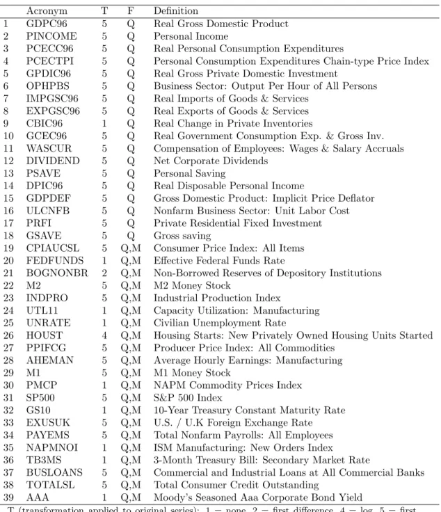
We apply the PPT and KP models to thirty-nine quarterly and twenty-one monthly series for the USA (listed in Table 2) which are among the most important macroeconomic variables. Twenty-one quarterly series are obtained by aggregation of the corresponding monthly series, The remaining eighteen quarterly series are not available at the monthly frequency. The sample period is 1959, first month (or quarter), till 2011, ninth month (or third quarter). As indicated in the table, we have transformed most series to growth rates or first differences, and in this we are proceeding as in the literature, see e.g. Stock and Watson (1996) and Bernanke, Boivin, and Eliasz (2005). We use AR(1) and AR(4) models in each regime, hence,
Ztin (1) contains an intercept and the lags of yt.
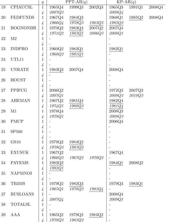
In Tables 3-5, we report the break dates found in the PPT-AR(1) and AR(4) models (called PPT1 and PPT4 hereafter), and similarly KP-AR(1) and AR(4) models (KP1 and KP4), using the complete sample. The reported break dates are medians of posterior distributions. We find no break in nine quarterly series (numbered 6, 14, 18, 22, 24, 26, 31, 35, 38) out of thirty-nine both with PPT and KP (irrespective of the lag order), in six other series
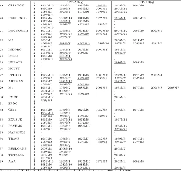
with PPT (2, 3, 5, 10, 11, 30), and in two other series (32, 39) with KP; see Tables 3 and 4. Three monthly series (26, 31, 35) out of twenty-one have no break both by PPT and KP, and one more (24) by KP. Three series (22, 24, 38) have breaks when used at the monthly frequency, but no break at the quarterly frequency. More generally, more breaks are obtained with monthly than quarterly series (compare Tables 4 and 5).
No quarterly series has more than three breaks, and few – seven by PPT, three by KP – have three breaks. On the contrary, ten monthly series have at least four breaks by one of the four models (PPT1, PPT4, KP1, KP4). PPT models generate more breaks than KP especially for the monthly series: medians of detected breaks are 3 by PPT, for both lag orders, but 1 for AR(1) and 0 for AR(4) with KP. This is due partly to the occurrence of breaks at close dates in eleven monthly series, a phenomenon observed only in two quarterly series.
For quarterly series, KP models detect more breaks towards the end of the sample than PPT: considering globally all four PPT and KP models, there are 16 such cases if we define, with some arbitrariness, a break at the end of the sample as a break occurring at any date after 2006. For the monthly series, this does not hold: there are 4 cases where a KP model detects a break after 2006 and PPT does not, and also 4 cases where PPT detects such a break but KP does not. Hence if there is a piling up problem for KP due to the use of a geometric prior (see discussion in section 2.3), it is linked to the quarterly series. It may be the case that with monthly series, break detection being more powerful due to more data, and the piling up problem is attenuated.
Several series have a break in the period 1980-1986 (see the underlined dates in the tables). These breaks correspond (for macroeconomic series) to what has been named the great moderation, with a decrease in the variance of the error term. For interest rates (series 20, 32, 36, 39), we observe breaks in 1979 (except for series 20) and at a date between 1982 and 1984; these correspond more or less to the the Volcker period at the Fed. The 1979 break for such series corresponds to a large increase in the estimated variance of the error terms.
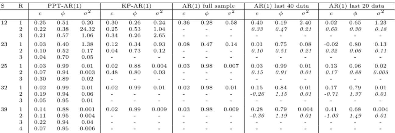
To illustrate the parameter estimates of PPT and KP models, Table 6 provides the pos-terior means of the parameters of the AR(1) equations of each regime for a few series. The table also reports the estimates when no break is allowed on the full sample, and estimates on subsamples. These results illustrate that the most sensitive parameter is the variance of
the error term. The constant term changes also as a consequence of some level changes in the data of some series. The autoregressive coefficient (φ) is more stable, with some exceptions, illustrated by series 23. For this series (the growth rate of industrial production), using the PPT results, the first regime (ending in 1960Q3) has the highest variability (σ2
), the lowest persistence and average level (estimated asc divided by 1−φ). The third regime, starting in 1983Q1, corresponds to the lowest variability, the highest persistence, and an average growth rate between those of the other two regimes. The third regime corresponds to the great moderation period, except that a break is not detected by PPT in 2008. KP finds only two regimes, with a break in 1982Q1. The estimated parameters of the second regime in KP are close to those of the third regime in PPT, and like for PPT, its error variance estimate is much lower than in the previous regime.
We do not report break dates for the GK models, since these models generate much more breaks than PPT and KP. This is mainly a consequence of using an independent Bernouilli prior for the sequence of state variables st, instead of a Markov chain structure.
In summary, there is evidence that macroeconomic series are subject to breaks since about three quarters of our series have at least one break when modeled by structural break models.
4
Results of Forecasting Evaluations
For each series listed in Table 2, we carry out a recursive forecasting exercise for the final (approximately) sixty percent of the observations: we first estimate the models with an initial sample consisting of (approximately) forty percent of the data, and we forecast at the horizons
h equal 1 and 4 for quarterly data, and 1 and 12 for monthly data. Then we add one data point, estimate and forecast again, until the end of the data. Thus for quarterly data, we have 83 in-sample observations at the start (1959Q1-1979Q4), and 127 in the forecast period, and for monthly data these numbers are 251 (1959M1-1979M12) and 381.6
For h > 1, our forecasts are iterated (see, e.g., Marcellino, Stock, and Watson (2006) for a motivation for use of iterated over direct forecasts).
Our forecast metrics are RMSE and the average of log predictive likelihoods (APL). RMSE
6Our forecast evaluation exercise requires us to estimate each model for 60 series; for 39 quarterly series, the recursive forecast evaluation requires that we estimate each model 126 times, and for 21 monthly series, 380 times, for a total of 30,360 estimations per model. For some break models, this takes a lot of time.
is based the predictive median as point forecast. The predictive likelihood is the predictive density evaluated at the observed outcome. This is estimated by a nonparametric kernel smoother using draws from the predictive simulator.
We discuss the results based on the RMSE criterion in subsection 4.1, and in subsection 4.2 the results based on the APL criterion. We are interested in three questions:
Question 1: How does the forecasting performance differ between break models and no-break models?
Question 2: How does the forecasting performance differ between break models?
Question 3: How does the forecasting performance differ between lag orders?
For each question, we shall also comment how the forecasting performance differ between quarterly and monthly series, whenever this is relevant.
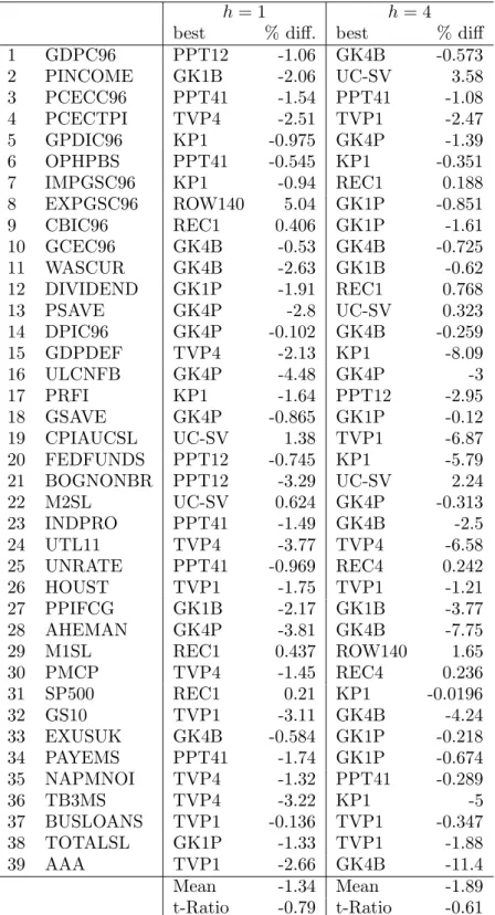
4.1 RMSE Results
We provide in Table 7 the list of the best model for each quarterly series, together with the relative performance of the best break model with respect to the best no-break model. The same type of information is provided in Table 8 for the monthly series.
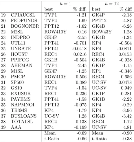
For the quarterly series: at horizon one, the break models are the best in 85 percent of all series (8 series for PPT, 3 for KP, 12 for GK, and 10 for TVP). At horizon four, the break models forecast better in 80 percent (3 series for PPT, 5 for KP, 17 for GK, and 6 for TVP). Hence, as the horizon increases, it appears that the performance of break models decreases slightly, while the KP and GK models increase their share at the expense of PPT and TVP. For the monthly series: the break models perform best in 67 percent of the series at both horizons, but the share of KP and GK models also increases with the horizon, at the expense of PPT and TVP.
Note that these scores do not take account of the magnitude of the differences of the RMSE between the different models (for this see below).
With the results in Tables 7 and 8, we can answer the three questions about the forecasting performance of the different models.
Question 1: We compare the best break model RMSE value to the best no-break model value, see columns ”% diff.” in the tables. For example, a value of -3 (+3) means that the
best break (no-break) model has its RMSE three percent smaller (larger) than the RMSE of the best no-break (break) model. Although for a high proportion of the series the differences are negative, they are nevertheless generally small, by what we mean they are less than five percent.7
Exceptions occur only for quarterly series: at horizon one, series 8 (in favor a no-break model); at horizon 4, series 15, 19, 20, 24, 36, and 39 (all in favor of break models).
Significance tests for the nullity of the mean of the differences8
are insignificant at the ten percent level for the two forecast horizons at each frequency (see reported t-statistics in the last rows of the tables). In brief, there is some weak evidence in our results that break models perform a little better than no-break models.
Question 2: The relative differences (in percent) between the RMSE of the different models for forecasts at horizons 1 and 4 (quarterly series) or 12 (monthly) are shown in Tables 5-12 of the TA. For example, the value –1.93 of quarterly series 1 for a comparison of PPT12 and KP1 at horizon 1 (see Table 5 of TA) means that PPT12 is performing better than KP1 by almost two percent.
For most series, the differences are small, but there are a few cases where they are large. For example, at horizon 1, for quarterly series 15, 30, 35 and 38, in the comparisons involving GK1B and GK4B, the ratios indicate that GK1B and GK4B is forecasting far away from the realizations; for series 21, there is also a number of large differences (around 50 percent), and the culprits are TVP1, TVP4, and KP4. For monthly series, more series have large differences, e.g. at horizon 1, series 20, 21, 25, 32, 35, 36 in comparisons involving GK1B and GK4B; series 21 in comparisons involving TVP1 and TVP4; series 36, 38, 39 in comparisons involving KP1.
Means and t-tests of significance of the means of the differences for each model comparison (like for Question 1) are given at the bottom of each column of the tables. In computing these statistics, we have eliminated the large differences (as shown in the tables)
7The choice of five percent as the frontier between small and large is of course arbitrary, and not necessarily sensible form an economic perspective. For example, for financial returns, five percent is a lot even at the quarterly frequency. Using an economic criterion to fix a threshold would require to define different criteria for different series and would render the comparison between the series difficult and also arbitrary to some extent. 8The test is based on the assumption that the 39 observed values of column 4 of Table 7 (as an example) are random draws of a common distribution with meanµ. The tested hypothesis is ”µ= 0” (versusµ6= 0). The test statistic (-0.79), equal to the sample mean (-1.34) divided by the sample standard deviation (1.69) of the 39 values, is asymptotically standard normal under the null hypothesis.
Judging by the means (at the bottom of the tables), for quarterly series, at horizons 1 (Table 5 of TA) and 4 (Table 7 of TA), KP1 performs better on average than the other models (PPT12, GK1B, GK1P, TVP1); PPT12 performs better than GK1P, GK1B, TVP1; GK1P dominates GK1B. TVP1 dominates GK1B and is dominated by GK1P at horizon 1, while at horizon 4, TVP1 surpasses GK1P and is surpassed by GK1B. For models using 4 lags, on average, at horizon 1 (Table 6 of TA) , PPT41 dominates the other models (KP4, GK4B, GK4P, TVP4); KP4 dominates TVP4, G4KB and GK4P; TVP4 performs better than both GK models and GK4P surpasses GK4B. At horizon 4 (Table 8 of TA), both GK models dominate TVP4, GK4P performs better than GK4B, PPT41 and KP4 perform quasi-equally, and both dominate the other models. However, the t-statistics are all insignificant at 10 percent in Tables 5-8 of the TA; this remains true if we do not trim the extreme values.
For monthly series, at horizon 1 (Table 9 of TA) , PPT12 performs better on average than KP1, GK1B, GK1P, TVP1; TVP1 dominates KP1, GK1P, GK1B; GK1P dominates KP1 and GK1B, and GK1B surpasses KP1. At horizon 12 (Table 11 of TA) , the results differ slightly: KP1 and GK1B dominate GK1P. For AR(4) models, at horizon 1 (Table 10 of TA), KP4 dominate the other models (PPT41, GK4B, GK4P, TVP4); PPT41 surpasses GK4B, GK4P, TVP4; TVP4 dominates both GK models, and GK4P surpasses GK4B. At horizon 12 (Table 12), TVP4 dominates the other models (PPT41, KP4, GK4B, GK4P); PPT41 surpasses KP4, GK4P and GK4B; KP4 dominates both GK models, and GK4P surpasses GK4B. Again, no
t-statistic (with or without trimming) is significant at 10 percent in Tables 9-12 of the TA. In summary, on average (across series), the results do not indicate that a subset of models performs better than the other, on the basis of thet-tests. However, judging by the average differences only, the KP, PPT and TVP models perform better than the GK models. This result holds after elimination of the large individual differences and thus are not due to the trimming we have applied. Combined with the fact that the models that provoke the large differences in some series is in almost all cases the GKxB model, we conclude that the KP, PPT and TVP models should be considered as the most useful class of break models, when evaluating forecasts by the RMSE criterion.
Question 3: The relative differences (in percent) between the RMSE of the different models for forecasts at all horizons are reported in Table 13-16 in the TA.
computed mean differences vary in sign and allt-statistics are insignificant at 10 percent. For no-break rolling window models, the computed mean differences are negative at all horizons (with two exceptions for RO110Y/RO410Y, in Tables 15 and 16 of the TA), suggesting that models with one lag tend to perform better. However, this evidence is weak, since the t -statistics reveal that the mean differences are not significant at the 10 percent level, both for quarterly and monthly series, and for all horizons.
4.2 APL Results
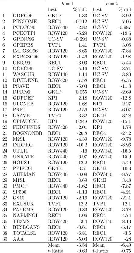
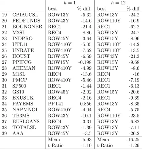
We list the best model for each quarterly and monthly series, respectively in Tables 9 and 10, together with the relative performance of the best break model with respect to the best no-break model.
For the quarterly series, at both horizons the no-break models perform better than the break models in roughly 80 percent of the series. The RO models have the highest share: 54 percent (21 series) at horizon 1 and 36 percent (14 series) at horizon 4. They are followed by the REC models (21 and 26 percent). Among the RO models, RO120 (1 lag, 20 observations per window) appears most often (12 series at horizon 1, and 10 at horizon 4). Given the dominance of RO120, models with 1 lag dominate models with 4 lags, but less so at horizon one than four.
For the monthly series, the domination of no-break models is very strong (95 percent at horizon 1, 100 at horizon 12, with a strong dominance of rolling window (RO) models at both horizons. At horizon 1, the RO models with 4 lags dominate those with one lag (12 against 2), while the reverse happens at horizon 12 (1 against 14). There is no clear pattern for the effect of the window size.
These scores do not take account of the magnitude of the differences of the APL between the different models (for this see question 1 below) but suggest that RO models are dominating the other models by far.
With the results in Tables 9 and 10, we can answer the three questions about the fore-casting performance of the different models.
Question 1: We compare the best break model APL value to the best no-break model value, see columns ”% diff.” in the tables. For example, a value of +4 (-4) means that the best break (no-break) model has its APL four percent larger than the APL of the best no-break
(break) model.
For a high proportion of the series the differences are negative, as our discussion just above has illustrated. They are larger than for the RMSE results: the average difference for quarterly data at horizon 1 is -3.5, and at horizon 4, it is -6.5. For monthly data, the mean differences are larger (-5.9 and -16.3) and also increase with the horizon. Nevertheless, the
t-statistics are insignificant at 10 percent. In brief, there is weak evidence in our results that the no-break models (especially RO) perform better than break models. Exceptions occur for the quarterly series numbered 6, 18, 27 and 33 at both horizons, and for a few other series at one horizon (series 1, 14, 16, 19, 20, 29). For monthly series, there is on exception only at horizon 1 (series 34).
Question 2: The relative differences (in percent) between the APL of the break models for forecasts at horizon one are shown in Tables 21-28 of the TA. For example, the value 28 for the quarterly series 1 (see Table 21 of TA) for the comparison GK1P/GK1B means that the APL of GK1P exceeds the APL of GK1B by 28 percent. The differences vary a lot, and there are a few cases where they are very large. The large differences occur mainly for series 21, 24-26, 30, 35 (plus 32 and 39 with monthly data) and in comparisons involving the TVP and GK models. Thus we have trimmed the statistics (as shown in the Tables) to avoid the influence of extreme values of the differences.
Judging by the means (at the bottom of the tables), for quarterly series, at horizon 1, KP1 performs better on average than the other models (PPT12, GK1B, GK1P, TVP1); PPT12 performs better than GK1P, GK1B, TVP1; GK1P dominates GK1B, and TVP1 dominates both GK models. For models using 4 lags, on average, KP4 dominates the other models (PPT41, GK4B, GK4P, TVP4); PPT14 dominates TVP4, G4KB and GK4P; TVP4 performs better than both GK models and GK4P surpasses GK4B. At horizon 4, the results are of the same kind. However, thet-statistics are insignificant at 10 percent in Tables 21-24 of the TA, except in the comparison PPT41/KP4 at horizon 4 (see Table 24 of the TA).
For monthly series, at horizon 1, PPT12 performs better on average than KP1, GK1B, GK1P, TVP1; KP1 dominates on average GK1P, GK1B, TVP1; GK1P dominates GK1B, and TVP1 surpasses both GK models. For AR(4) models, the rankings are similar, except that GK4B dominates GK4P. At horizon 12, for AR(1) models, the results differ from those for horizon 1 only by the fact that KP1 dominates PPT12. For AR(4) models, KP4 dominates
the other models, PPT41 dominates TVP4 and both GK4 models, GK4B surpasses GK4P and TVP4, and TVP4 performs better than GK4P. Again, not-statistic (after trimming) is significant at 10 percent in Tables 25-28 of the TA, but if trimming is not applied, all statistics remain insignificant.
In brief, on average (across series), the results do not indicate that a subset of models performs better than the other, on the basis of thet-tests. However, judging by the average differences only, the KP and PPT models perform better than the GK and TVP models. This result holds after elimination of the large individual differences and thus are not due to the trimming we have applied. Combined with the fact that the models that provoke the large differences in some series are in almost all cases the GK and TVP models, we conclude that the KP and PPT models should be considered as the most useful class of break models, when evaluating forecasts by the APL criterion.
Question 3: The relative differences (in percent) between the APL of the different models for forecasts at horizons 1 and 4 are reported in Tables 29-32 of the TA.
For break models, the computed mean differences do not reveal a systematic dominance (on average) of one lag order, and thet-statistics are all insignificant at the 10 percent level. The mean differences are in most cases larger at the higher horizons (4 for quarterly series, 12 of monthly).
For no-break models models, at the larger horizons, all the mean differences are positive, thus in favor of models with 1 lag, but only one is significant (see RO120/RO420 in Tables 30 of the TA). At horizon 1, no systematic pattern emerges andt-statistics are all insignificant at 10 percent.
4.3 Discussion of Previous Results
For the APL criterion, we find that the no-break models, especially rolling AR models, perform better on average than the break models. For the RMSE criterion, we find some evidence in favor of break models. Why this difference?
The APL criterion takes into account the whole shape of the predictive density. This is not Gaussian despite the assumption of normality conditional on the parameters, because it is integrated with respect to a posterior distribution that is not symmetric. However our predictive densities are very moderately skewed, especially for forecasts at short horizons.
Therefore, we can summarize the shape of our predictive by their standard deviation. The RMSE results indicate that in terms of the location of the point forecasts in the support of the predictive densities, the two kinds of models (break/no-break) are roughly equivalent on average (of course, individual exceptions occur). Thus the differences in the APL results is, at least partly, due to differences in the standard deviations of the predictive densities. *** DO WE HAVE EVIDENCE IN THE RESULTS THAT SUPPORTS OUR EXPLANA-TION? NOT FROM TABLE 6...***
5
Sensitivity Analyses
We perform two sensitivity checks. The first is with respect to the forecast period: we focus on the data starting in 2007, which corresponds more or less to the beginning of the global financial crisis, until the end of the sample (i.e. 19 observations for quarterly series, and 57 monthly observations). The second check concerns the influence of the prior used in the break models.
5.1 Forecast performance since 2007
These results were obtained with the same prior as in the previous section. For the RMSE criterion, break models perform better than no-break models in 74 percent of quarterly series at horizon 1 and 59 at horizon 4. These values are a little lower than for the corresponding results (85 and 77) reported in the previous section. The corresponding proportions are 62 (horizon 1) and 86 (horizon 12) for monthly series (versus 67 in the previous section at both horizons). The corresponding mean differences are negative but small, and the t-statistics (reported in Table 11) are insignificant, as in the previous section.
For the APL criterion, we find that no-break models perform better than break models in 63 percent of series at both horizons for quarterly series (instead of 80 in the previous section), and in 95 percent for monthly series at both horizons, much like in the previous section. The mean differences are insignificant, though for monthly series the mean differences are close to minus 10 percent and one of them is close to being significant at 10 percent.
In summary, the results for the post-2006 forecast sample are broadly similar to those for the post-1979 forecast sample.
5.2 Impact of the prior for break models
In Bayesian inference, it is good practice to assess the sensitivity of the results with respect to the informative content of the prior. Thus we have computed all the results with different sets of prior hyperparameters. One set implies a more informative prior (PRIOR M), and the other a less informative prior (PRIOR L) than our intermediate prior (PRIOR I) used for getting all the results reported in the previous (sub)sections. The parameter values of PRIOR I are given at the end of subsection 2.2. Due to space limitations, we report briefly the results for AR(1) PPT and KP models (PPT12 and KP1).
All our priors (M, I, L) imply that the unconditional prior expectations are equal to zero for the regression coefficients of the AR(1) or AR(4) equations in each regime since
E(βj) =E[E(βj|β0)] =E(β0) and the latter is set to zero. They imply non-existing second
moments for the regression coefficients because V ar(βj) =V ar[E(βj|β0)] +E[V ar(βj|β0)] = V ar(β0) +E(B0) andE(B0) is not finite due to setting the degrees of freedom of the Wishart prior to m+ 1, withm= 2 for AR(1) and 5 for AR(4). However V ar(β0) is set toVβ =cIm
withc = 1 in PRIOR I and by changing the value of c, we can change the tightness of the prior on the regression coefficients.
In PRIOR L, we setc= 100, implying standard deviations equal to 10 forβ0, that is ten times larger than the corresponding value in PRIOR I (which has c = 1). We are also less informative on error variances of AR equations by setting ρ= 0.01 and d= 0.01 (instead of 0.1 for both in PRIOR I) in the PPT model. In the KP model, we setVω = 100 (instead of 1) andκ1=κ2 = 0.01 (instead of 0.5).
In PRIOR M, we setc= 0.01Im, implying a more precise prior (with standard deviations
of 0.1) than in PRIOR I. For the other parameters of the prior, the values are the same as in PRIOR I.
Computed by simulation, the highest prior density interval of ninety percent level for each regression coefficient is equal to (−17,+17) for PRIOR L, (−3.9,+3.9) for PRIOR I, and (−2.6,+2.6) for PRIOR M. Notice that if c is set to a smaller value than 0.01, the last interval does not shrink due to the E(B0) term that is not finite. Compared to the precisions typically implied by the type of data and sample size we use, all these priors are little informative, but PRIOR L is substantially less tight than the other two, while PRIOR M is slightly more concentrated than PRIOR I. In Table 12, we summarize the difference
between the results with the three priors, for both criteria and for AR(1) specifications. For each series, horizon, and forecasting model (PPT12 and KP1), we compute the per-centage difference in each criterion value (RMSE and APL) of PRIOR M and PRIOR L relative to PRIOR I. Then we take the average of these values over all series and we test the significance of the mean. For example, thepositive mean of 0.51 for the RMSE criterion for PPT12 at horizon one indicates that on average the performance is better with PRIOR I than with PRIOR L, by half of a percent. The corresponding t-statistic (0.32) indicates that this is not significant even at the ten percent level. For the APL criterion, anegative mean such as−3.58 for KP1 at horizon one indicates a better performance with PRIOR I than PRIOR L.
For the RMSE criterion, the differences of performance are small on average, and statis-tically insignificant: the largest mean difference is at horizon 4 for PPT12 (2.21 percent in favor of PRIOR I relative to M). Except in one case, all mean differences are in favor of prior I.
For the APL criterion, all mean differences are in favor of prior I. The mean differences are small for PPT12 at both horizons in both comparisons, the largest (-1.98) being significant at 10%. For KP1, the mean differences are larger (over 3.5%), the largest one (-13.2%) being significant at 5%.
6
Conclusions
In this paper, we have compared various forecasting procedures which allow for structural breaks in a set of sixty US macroeconomic time series, quarterly and monthly. Our set of forecasting procedures is divided into two groups: ones which formally model the break process (KP, PPT , GK, and TVP) and those which do not (rolling and recursive window based forecasts, and UC-SV).
Our empirical results do not tell one single consistent story, but rather a variety of stories. Most importantly, we have added to the literature establishing the widespread existence of structural breaks in major macroeconomic time series. Our results also show the importance of using a forecasting method which allows for parameter change of some sort. However, perhaps unsurprisingly, we have not established that there is one single forecasting method that always is to be preferred. Each of our methods performs well in some cases, but not as
well in others.
In terms of RMSE, we find weak evidence in favor of a better performance of break models, with some advantage to KP and PPT. We find no evidence that these break models are harmful for individual series, so that we recommend to consider them as potentially useful forecasting models. They might also add value if forecast combination were considered, an issue that we leave for further research.
In terms of predictive likelihoods, it is often the case that rolling (fixed window) forecasts are better than approaches which formally model the break process. In Section 5.3, we have offered an explanation for this. However, it is worthwhile to expand on this finding. In an effort to produce automatic forecasting procedures, suitable for repeated use with many data sets, this paper has used very simple implementations of PPT, KP, and GK break models. In particular, for each series, we have used the same models (i.e. AR models), with the same prior (a relatively noninformative one) and the break process has been modeled in a very simple way. It is possible that these break models are not well-designed for use in such a black box fashion. For instance, we have imposed that breaks in AR coefficients and error variance occur at the same time. But in some of the series, it looks to be the case that having separate break processes for the error variance and regression coefficients would be useful (i.e. ensuring more parsimony by allowing breaks in the conditional variance but not in the conditional mean). Also, it is likely that calibrating priors on a case-by-case basis (or using more sophisticated hierarchical priors) could improve forecast performance. And, the hierarchical structures of the break models will tend to be of most use in more complicated forecasting models (e.g. involving many predictors or with VARs) where rolling or recursive forecasting methods can perform poorly (see, e.g., Korobilis and Koop (2010)) rather than simple univariate AR setups.
In sum, in this paper we have established the importance of structural breaks for fore-casting in many macroeconomic time series. However, we also recommend the careful devel-opment of appropriate structural break models on a case-by-case basis as opposed to use of an automatic procedure.
A potentially useful extension of our research will be to base the forecasts on models using other regressor variables than lags, and on multivariate models, noticing that Pettenuzzo and Timmermann (2011) have extended the PPT framework to such models.
References
Ang, A.,and G. Bekaert(2002): “Regime switches in interest rates,”Journal of Business
and Economic Statistics, 20, 163–182.
Bernanke, B., J. Boivin,andP. Eliasz(2005): “Measuring the Effects of Monetary
Pol-icy: A Factor-augmented Vector Autoregressive (FAVAR) Approach,” Quarterly Journal of Economics, 1(120), 387–422.
Chib, S. (1998): “Estimation and comparison of multiple change-point models,”Journal of
Econometrics, 86, 221–241.
Clark, T., and M. McCracken (2009): “Improving forecast accuracy by combining
re-cursive and rolling forecasts,”International Economic Review, 50, 363–395.
Clements, M.,and D. Hendry(1998): Forecasting economic time series. Cambridge
Uni-versity Press, Cambridge.
D’Agostino, A., L. Gambetti, and D. Giannone (2009): “Macroeconomic forecasting
and structural change,” ECARES working paper 2009-20.
Eklund, J., G. Kapetanios,and S. Price(2009): “Forecasting in the presence of recent
and recurring structural change,” Mimeo, Queen Mary University London, Department of Economics.
Gerlach, R., C. Carter,andR. Kohn(2000): “Efficient Bayesian Inference for Dynamic
Mixture Models,” Journal of the American Statistical Association, 95, 819–828.
Giordani, P.,and R. Kohn(2008): “Effcient Bayesian inference for multiple change-point
and mixture innovation models,”Journal of Business and Economic Statistics, 26, 66–77.
Koop, G., and S. Potter (2007): “Estimation and forecasting with multiple breaks,”
Review of Economic Studies, 74, 763–789.
(2009): “Prior elicitation in multiple change-point models,” International Economic Review, 50, 751–772.
Korobilis, D., and G. Koop (2010): “Forecasting inflation using dynamic model
Maheu, J., andS. Gordon(2008): “Learning, forecasting and structural breaks,”Journal of Applied Econometrics, 23, 553–583.
Marcellino, M., J. H. Stock, and M. W. Watson (2006): “A comparison of direct
and iterated multistep AR methods for forecasting macroeconomic time series,”Journal of Econometrics, 135, 499–526.
McCulloch, R., and R. Tsay (1993): “Bayesian Inference and Prediction for Mean and
Variance Shifts in Autoregressive Time Series,” Journal of the American Statistical Asso-ciation, 88, 968–978.
Meese, R., andJ. Geweke(1984): “A comparison of autoregressive univariate forecasting
procedures for macroeconomic time series,” Journal of Business and Economic Statistics, 2, 191–200.
Pesaran, M. H., D. Pettenuzzo, and A. Timmermann(2006): “Forecasting time series
subject to multiple structural breaks,” Review of Economic Studies, 73, 1057–1084.
Pesaran, M. H., and A. Timmermann (2007): “Selection of estimation window in the
presence of breaks,”Journal of Econometrics, 137, 134–161.
Pettenuzzo, D., and A. Timmermann (2011): “Predictability of stock returns and asset
allocation under structural breaks,”Journal of Econometrics, 164(1), 60–78.
Stock, J. H., and M. W. Watson(1996): “Evidence on structural instability in
macroe-conomic time series relations,” Journal of Business & Economic Statistics, 14, 11–30. (2007): “Why has U.S. inflation become harder to forecast?,” Journal of Money, Credit & Banking, 39, 3–33.
Table 1: Models used in the forecasting evaluations
Name Description
Break models (all series)
PPT12 PPT with geometric prior, AR(1), 2 breaks allowed in forecast period PPT41 PPT with geometric prior, AR(4), 1 break allowed in forecast period
KP1 KP with geometric prior, AR(1)
KP4 KP with geometric prior, AR(4)
GK1B Mixture innovation model, geometric prior, AR(1) GK4B Mixture innovation model, geometric prior, AR(4) GK1P Mixture innovation model, Poisson prior, AR(1) GK4P Mixture innovation model, Poisson prior, AR(4)
TVP1 Time-Varying Parameter AR(1) model
TVP4 Time-Varying Parameter AR(4) model
No-break models (quarterly series)
RO120 AR(1) estimated with rolling window of 5 years (20 observations) RO140 AR(1) estimated with rolling window of 10 years (40 observations) RO420 AR(4) estimated with rolling window of 5 years
RO440 AR(4) estimated with rolling window of 10 years
REC1 AR(1) estimated on expanding window
REC4 AR(4) estimated on expanding window
UC-SV Unobserved component model with stochastic volatility No-break models (monthly series)
RO13Y AR(1) estimated with rolling window of 3 years (36 observations) RO15Y AR(1) estimated with rolling window of 5 years (60 observations) RO110Y AR(1) estimated with rolling window of 10 years (120 observations) RO43Y AR(4) estimated with rolling window of 3 years
RO45Y AR(4) estimated with rolling window of 5 years RO410Y AR(4) estimated with rolling window of 10 years
REC1 AR(1) estimated on expanding window
REC4 AR(4) estimated on expanding window
Table 2: Variables used in forecast evaluation
Acronym T F Definition
1 GDPC96 5 Q Real Gross Domestic Product
2 PINCOME 5 Q Personal Income
3 PCECC96 5 Q Real Personal Consumption Expenditures
4 PCECTPI 5 Q Personal Consumption Expenditures Chain-type Price Index
5 GPDIC96 5 Q Real Gross Private Domestic Investment
6 OPHPBS 5 Q Business Sector: Output Per Hour of All Persons
7 IMPGSC96 5 Q Real Imports of Goods & Services
8 EXPGSC96 5 Q Real Exports of Goods & Services
9 CBIC96 1 Q Real Change in Private Inventories
10 GCEC96 5 Q Real Government Consumption Exp. & Gross Inv.
11 WASCUR 5 Q Compensation of Employees: Wages & Salary Accruals
12 DIVIDEND 5 Q Net Corporate Dividends
13 PSAVE 5 Q Personal Saving
14 DPIC96 5 Q Real Disposable Personal Income
15 GDPDEF 5 Q Gross Domestic Product: Implicit Price Deflator
16 ULCNFB 5 Q Nonfarm Business Sector: Unit Labor Cost
17 PRFI 5 Q Private Residential Fixed Investment
18 GSAVE 5 Q Gross saving
19 CPIAUCSL 5 Q,M Consumer Price Index: All Items
20 FEDFUNDS 1 Q,M Effective Federal Funds Rate
21 BOGNONBR 2 Q,M Non-Borrowed Reserves of Depository Institutions
22 M2 5 Q,M M2 Money Stock
23 INDPRO 5 Q,M Industrial Production Index
24 UTL11 1 Q,M Capacity Utilization: Manufacturing
25 UNRATE 1 Q,M Civilian Unemployment Rate
26 HOUST 4 Q,M Housing Starts: New Privately Owned Housing Units Started
27 PPIFCG 5 Q,M Producer Price Index: All Commodities
28 AHEMAN 5 Q,M Average Hourly Earnings: Manufacturing
29 M1 5 Q,M M1 Money Stock
30 PMCP 1 Q,M NAPM Commodity Prices Index
31 SP500 5 Q,M S&P 500 Index
32 GS10 1 Q,M 10-Year Treasury Constant Maturity Rate
33 EXUSUK 5 Q,M U.S. / U.K Foreign Exchange Rate
34 PAYEMS 5 Q,M Total Nonfarm Payrolls: All Employees
35 NAPMNOI 1 Q,M ISM Manufacturing: New Orders Index
36 TB3MS 1 Q,M 3-Month Treasury Bill: Secondary Market Rate
37 BUSLOANS 5 Q,M Commercial and Industrial Loans at All Commercial Banks
38 TOTALSL 5 Q,M Total Consumer Credit Outstanding
39 AAA 1 Q,M Moody’s Seasoned Aaa Corporate Bond Yield
T (transformation applied to original series): 1 = none, 2 = first difference, 4 = log, 5 = first difference of logged variable. F (frequency): Q = quarterly, M = monthly. Sample period (after data transformation): 1959M1-2011M9 (633 observations) or 1959Q1-2011Q3 (211 observations) Data source: St. Louis FRED database.
Table 3: Break dates based on full sample (quarterly data) q PPT-AR(q) KP-AR(q) 1 GDPC96 1 1983Q1 1983Q4 4 1982Q2 -2 PINCOME 1 - -4 - 2008Q3 3 PCECC96 1 - 1993Q3 4 - -4 PCECTPI 1 2006Q2 2008Q3 2010Q3 4 2007Q3 2008Q4 2010Q3 5 GPDIC96 1 - 1984Q3 2008Q3 4 - 1983Q4 6 OPHPBS 1 - -4 - -7 IMPGSC96 1 1986Q1 1986Q3 2008Q3 4 1984Q4 2007Q2 1986Q1 2008Q3 8 EXPGSC96 1 1978Q3 1979Q1 4 - 1979Q1 9 CBIC96 1 1979Q4 1977Q3 2009Q1 4 1977Q3 1980Q3 10 GCEC96 1 - 1973Q4 4 - -11 WASCUR 1 - 2000Q1 4 - -12 DIVIDEND 1 2004Q2 2005Q1 1973Q2 2004Q4 4 1990Q4 2003Q3 2004Q2 2004Q4 13 PSAVE 1 1998Q1 1998Q4 4 1996Q3 1998Q4 14 DPIC96 1 - -4 - -15 GDPDEF 1 1965Q4 1982Q2 1985Q2 4 1980Q1 1981Q2 16 ULCNFB 1 1983Q2 1999Q1 1983Q4 1999Q4 4 - -17 PRFI 1 1983Q1 2006Q1 1983Q3 2006Q2 2009Q3 4 1982Q2 2006Q1 1983Q2 2007Q1 18 GSAVE 1 - -4 -
-Break dates are defined as the first observation of the new regime, using the median of the posterior of the states. Underlined are break dates between 1980 and 1986.
Table 4: Break dates based on full sample (quarterly data) q PPT-AR(q) KP-AR(q) 19 CPIAUCSL 1 1965Q4 1999Q3 2002Q3 1965Q3 1991Q1 2008Q4 4 2007Q3 2008Q4 20 FEDFUNDS 1 1967Q4 1984Q3 1968Q1 1985Q2 2008Q4 4 1966Q4 1978Q3 1983Q3 1985Q2 21 BOGNONBR 1 1970Q2 1983Q4 2007Q2 2007Q4 4 1971Q2 1983Q1 2006Q3 2008Q1 22 M2 1 - -4 - -23 INDPRO 1 1960Q2 1983Q1 1982Q1 4 1960Q2 1981Q1 -24 UTL11 1 - -4 - -25 UNRATE 1 1983Q3 2007Q4 2008Q4 4 - -26 HOUST 1 - -4 - -27 PPIFCG 1 2006Q2 1972Q3 2007Q3 4 2007Q1 2008Q3 2010Q3 28 AHEMAN 1 1967Q2 1981Q4 1982Q4 4 1974Q1 1980Q3 1981Q4 29 M1 1 1978Q4 2008Q3 4 1978Q1 2008Q3 30 PMCP 1 - 2006Q4 4 - -31 SP500 1 - -4 - -32 GS10 1 1979Q2 1984Q2 -4 1978Q3 1983Q2 -33 EXUSUK 1 1967Q2 1967Q4 4 1966Q3 1967Q2 1970Q2 -34 PAYEMS 1 1983Q2 1984Q1 2008Q2 4 1982Q1 -35 NAPMNOI 1 - -4 - -36 TB3MS 1 1979Q2 1982Q3 1979Q3 1983Q1 4 1965Q1 1978Q2 1983Q4 -37 BUSLOANS 1 - 2008Q4 4 2007Q4 2009Q1 38 TOTALSL 1 - -4 - -39 AAA 1 1965Q2 1979Q2 1984Q2 -4 1978Q3 1983Q2
Table 5: Break dates based on full sample (monthly data) q PPT-AR(q) KP-AR(q) 19 CPIAUCSL 1 1965M10 1973M4 1973M8 1982M5 1965M9 2005M6 1 1990M9 1996M8 1999M2 2005M5 2004M12 4 1965M4 1973M1 1973M6 1990M7 2004M12 4 1998M11 -20 FEDFUNDS 1 1962M5 1966M10 1974M6 1975M2 1985M1 2008M10 1 1979M8 1982M7 1989M3 -4 1962M2 1996M7 1979M5 1982M5 -4 1987M10 -21 BOGNONBR 1 1970M1 1983M8 2001M7 2007M10 2007M12 2008M9 2009M5 4 1959M5 1969M10 1983M8 2001M4 2007M12 4 2001M8 2007M7 -22 M2 1 2000M1 2000M3 2011M7 4 1969M8 1982M8 1982M11 1999M10 1970M2 2000M5 2011M6 4 2001M1 -23 INDPRO 1 1960M1 1984M1 2008M6 2009M4 1984M3 4 1959M11 1983M9 2008M1 1982M3 24 UTL11 1 1960M3 1984M1 -4 1959M11 1982M10 -25 UNRATE 1 - 1986M3 2008M5 4 - -26 HOUST 1 - -4 - -27 PPIFCG 1 1972M10 1975M1 1981M6 2000M11 1972M10 1975M2 2000M4 4 1972M7 1974M8 1982M8 2005M3 1972M7 2005M8 28 AHEMAN 1 1968M7 1981M12 1982M5 4 1959M4 1960M3 1982M2 -29 M1 1 1965M1 1979M2 1988M5 2001M7 1965M4 1979M8 2001M8 2008M7 1 2001M10 2008M5 -4 1979M7 1981M10 2001M3 -30 PMCP 1 2004M12 2005M3 4 2004M9 -31 SP500 1 - -4 - -32 GS10 1 1965M9 1979M5 1979M8 1982M8 1966M4 1979M8 1 1982M11 1988M4 -4 1965M6 1979M4 1982M4 1982M7 -33 EXUSUK 1 1967M9 1967M12 1971M6 1967M11 4 1967M5 1967M8 1971M3 -34 PAYEMS 1 1960M4 1983M6 1983M10 1983M12 4 1960M1 1983M7 1983M12 35 NAPMNOI 1 - -4 - -36 TB3MS 1 1960M6 1966M4 1979M7 1982M8 1969M3 1979M4 4 1960M2 1966M1 1979M4 1982M4 1966M9 1973M8 4 1982M6 1985M4 -37 BUSLOANS 1 2008M8 2008M10 2008M7 4 2008M5 2008M9 -38 TOTALSL 1 2002M2 2008M3 2008M7 4 2010M9 -39 AAA 1 1959M12 1963M1 1965M10 1979M7 2002M4 2008M8 1 1982M6 1982M10 1988M4 4 1965M9 1979M4 1982M12 2002M3
Table 6: Posterior means of AR(1) models
S R PPT-AR(1) KP-AR(1) AR(1) full sample AR(1) last 40 data AR(1) last 20 data
c φ σ2 c φ σ2 c φ σ2 c φ σ2 c φ σ2 12 1 0.25 0.51 0.20 0.30 0.26 0.24 0.36 0.28 0.58 0.40 0.19 2.40 0.02 0.65 1.23 2 0.22 0.38 24.32 0.25 0.53 1.04 - - - 0.33 0.47 0.21 0.60 0.30 0.18 3 0.21 0.57 1.06 0.34 0.26 2.65 - - - -23 1 0.03 0.40 1.38 0.12 0.34 0.93 0.08 0.47 0.14 0.01 0.75 0.08 -0.02 0.80 0.13 2 0.10 0.52 0.17 0.04 0.73 0.12 - - - 0.10 0.51 0.21 0.32 0.06 0.11 3 0.04 0.70 0.05 - - - -25 1 0.03 0.99 0.01 0.02 0.88 0.004 0.03 0.98 0.007 0.03 0.99 0.01 0.13 0.96 0.02 2 0.07 0.94 0.003 0.48 0.80 0.03 - - - 0.15 0.91 0.01 0.17 0.88 0.003 3 0.30 0.89 0.02 - - - -32 1 0.02 0.99 0.01 0.02 0.99 0.01 0.02 0.98 0.01 0.15 0.84 0.01 0.17 0.79 0.01 2 0.19 0.94 0.06 - - - -0.26 1.15 0.01 -0.71 1.37 0.01 3 0.05 0.95 0.01 - - - -39 1 0.14 0.88 0.001 0.02 0.99 0.009 0.03 0.98 0.009 0.28 0.79 0.004 0.41 0.68 0.004 2 0.11 0.95 0.004 - - - -0.36 1.19 0.01 -1.03 1.49 0.01 3 0.22 0.94 0.04 - - - -4 0.07 0.95 0.006 - - -
-S = series number (see Table 2); R = regime number. Each AR(1) is writtenyt=c+φyt−1+σǫt. Two
estimations are reported in the block ”AR(1) last 40 data”: on the first row, the results are for the last 40 points of the full sample, on the second row (in italics), they are for the last 40 points ending in 1979Q4 (i.e. at 60 percent of the full sample). Similar for ”AR(1) last 20 data”.
Table 7: RMSE relative performance of best forecasting models on last sixty percent of sample (quarterly data)
h= 1 h= 4
best % diff. best % diff
1 GDPC96 PPT12 -1.06 GK4B -0.573 2 PINCOME GK1B -2.06 UC-SV 3.58 3 PCECC96 PPT41 -1.54 PPT41 -1.08 4 PCECTPI TVP4 -2.51 TVP1 -2.47 5 GPDIC96 KP1 -0.975 GK4P -1.39 6 OPHPBS PPT41 -0.545 KP1 -0.351 7 IMPGSC96 KP1 -0.94 REC1 0.188 8 EXPGSC96 ROW140 5.04 GK1P -0.851 9 CBIC96 REC1 0.406 GK1P -1.61 10 GCEC96 GK4B -0.53 GK4B -0.725 11 WASCUR GK4B -2.63 GK1B -0.62 12 DIVIDEND GK1P -1.91 REC1 0.768 13 PSAVE GK4P -2.8 UC-SV 0.323 14 DPIC96 GK4P -0.102 GK4B -0.259 15 GDPDEF TVP4 -2.13 KP1 -8.09 16 ULCNFB GK4P -4.48 GK4P -3 17 PRFI KP1 -1.64 PPT12 -2.95 18 GSAVE GK4P -0.865 GK1P -0.12 19 CPIAUCSL UC-SV 1.38 TVP1 -6.87 20 FEDFUNDS PPT12 -0.745 KP1 -5.79 21 BOGNONBR PPT12 -3.29 UC-SV 2.24 22 M2SL UC-SV 0.624 GK4P -0.313 23 INDPRO PPT41 -1.49 GK4B -2.5 24 UTL11 TVP4 -3.77 TVP4 -6.58 25 UNRATE PPT41 -0.969 REC4 0.242 26 HOUST TVP1 -1.75 TVP1 -1.21 27 PPIFCG GK1B -2.17 GK1B -3.77 28 AHEMAN GK4P -3.81 GK4B -7.75 29 M1SL REC1 0.437 ROW140 1.65 30 PMCP TVP4 -1.45 REC4 0.236 31 SP500 REC1 0.21 KP1 -0.0196 32 GS10 TVP1 -3.11 GK4B -4.24 33 EXUSUK GK4B -0.584 GK1P -0.218 34 PAYEMS PPT41 -1.74 GK1P -0.674 35 NAPMNOI TVP4 -1.32 PPT41 -0.289 36 TB3MS TVP4 -3.22 KP1 -5 37 BUSLOANS TVP1 -0.136 TVP1 -0.347 38 TOTALSL GK1P -1.33 TVP1 -1.88 39 AAA TVP1 -2.66 GK4B -11.4 Mean -1.34 Mean -1.89 t-Ratio -0.79 t-Ratio -0.61
See Table 1 for model definitions. The ”%diff” are computed as [(small-est RMSE across the break models/small[(small-est RMSE across the no-break models)-1]x100. Results computed from Tables 1 and 2 of the TA.