QR DECOMPOSITION FRAMEWORK FOR EFFICIENT IMPLEMENTATION OF LINEAR SUPPORT VECTOR MACHINES USING DUAL ASCENT
A Thesis by
VENKATA NAGA SAI PRITHVI SAKURU
Submitted to the Office of Graduate and Professional Studies of Texas A&M University
in partial fulfillment of the requirements for the degree of MASTER OF SCIENCE
Chair of Committee, Rabi N Mahapatra Co-Chair of Committee, Raktim Bhattacharya Committee Member, Vivek Sarin
Head of Department, Dilma Da Silva
August 2016
Major Subject: Computer Science
ABSTRACT
Support Vector Machines (SVMs) is a popular method to solve standard machine learning tasks like classification, regression or clustering. There are many algorithms to solve the linear SVM classification problem. However, only a few algorithms are optimized on both per iteration cost and convergence. While fast convergence is essential for solving any optimization problem, per iteration cost is critical in resource-limited environments like dedicated embedded solutions for machine learn-ing problems. In this thesis, we propose a novel approach to solve large-scale linear SVM classification problems. The proposed algorithm has low per iteration cost and also converges faster than existing state-of-art solvers.
There are two significant contributions from this thesis. First, we analyzed and improved the performance of the dual ascent (DA) algorithm, which would serve as the optimizing engine for solving SVM classification problem. An analytical model to evaluate the optimum step size and synchronization period for solving a generic quadratic programming optimization problem using DA is presented. Second, we implement SVM using the improved Dual Ascent algorithm. We also introduce a novel approach to tackle low dimensional classification problems of large data sizes via QR decomposition technique.
ACKNOWLEDGEMENTS
First and foremost I would like to express my gratitude to my advisor Dr. Rabi Mahapatra for the continuous support and motivation throughout the course of re-search. His experience and knowledge has taught me a lot and made be a better researcher. Besides my advisor, I would like to thank my committee co-chair Dr. Raktim Bhattacharya and committee member Dr. Vivek Sarin for their valuable ideas and inputs without which this research would not have been possible.
I would like to specially thank my fellow labmate Jyotikrishna Dass for all the stimulating discussions, long meetings relating to the research. These discussions prompted me to widen my research from various perspectives. Special thanks to Dr. Kooktae Lee for his insightful thoughts on the research and his motivating interactions.
I would also like to ackowledge Texas A&M High Performance Research Com-puting (http://hprc.tamu.edu/) for the comCom-puting platform and the resources used in performing necessary experiments.
Last but not the least I would like to express my heartfelt thanks to my parents, my sister and my friends for their love, encouragement and support throughout.
NOMENCLATURE
ADMM Alternating Method of Multipliers AWS Amazon Web Services
DA Dual Ascent Algorithm DCD Dual Coordinate Descent EC2 Elastic Cloud Compute HPC High Performance Computing IB InfiniBand interconnect IoT Internet of Things LAN Local Area Network
LSDA Lazy Synchronized Dual Ascent MPI Message Passing Interface QP Quadratic Programming QR QR decomposition
SMO Sequential minimization optimization SVM Support Vector Machines
TABLE OF CONTENTS Page ABSTRACT . . . ii ACKNOWLEDGEMENTS . . . iii NOMENCLATURE . . . iv TABLE OF CONTENTS . . . v
LIST OF FIGURES . . . vii
LIST OF TABLES . . . x
1. INTRODUCTION . . . 1
2. RELATED WORK . . . 4
2.1 Lazily Synchronized Dual Ascent . . . 4
2.2 QR-SVM Framework . . . 5
3. LAZILY SYNCHRONIZED DUAL ASCENT . . . 7
3.1 Introduction - Dual Ascent . . . 7
3.1.1 Dual Decomposition . . . 8
3.1.2 Quadratic Programming Using Dual Ascent . . . 9
3.2 Proposed - Lazily Synchronized Dual Ascent . . . 11
3.2.1 Stopping Criteria of LSDA . . . 12
3.2.2 Stability of LSDA . . . 13
3.2.3 Convergence of LSDA . . . 14
3.2.4 Optimal Synchronization Period . . . 15
3.2.5 Theoretical Speedup of LSDA . . . 18
3.2.6 LSDA in a Single Processor Environment . . . 20
3.3 Experimental Results . . . 21
3.3.1 Implementation . . . 21
3.3.2 Experimental Setup and Hardware . . . 22
3.3.3 Results and Discussion . . . 23
4. QR - SVM . . . 34
4.1 Introduction - Support Vector Machines . . . 34
4.1.1 Mathematical Formulation . . . 36 4.2 Linear SVM . . . 40 4.2.1 Challenges . . . 42 4.3 Proposed QR-SVM . . . 42 4.3.1 Motivation . . . 42 4.3.2 QR-SVM Formulation for L2-SVM . . . 43 4.3.3 Benefits of QR-SVM . . . 44
4.4 Optimization Using Dual Ascent . . . 46
4.4.1 Optimal Step Size of Optimization Algorithm . . . 49
4.5 Complexity Analysis . . . 51
4.6 Experiments . . . 51
4.6.1 Results and Discussion . . . 52
4.7 Conclusion . . . 58
5. CONCLUSION AND FUTURE WORK . . . 59
5.1 Future Scope . . . 59
REFERENCES . . . 61
APPENDIX A. QR DECOMPOSITION . . . 67
LIST OF FIGURES
FIGURE Page
3.1 Process distribution of a separable QP problem. . . 10 3.2 Distribution of iterations of dual ascent algorithm with a
synchroniza-tion period P . . . 12 3.3 Optimal synchronization period, P∗ as derived in equation (3.16).
Here, A1 = |1−λ(M)P| and A2 = |1−λ¯(M)P|. . . 17 3.4 Theoretical speedup of LSDA when compared with conventional DA
algorithm. . . 20 3.5 Block schematic of EOS cluster. Source: Texas A&M High-Performance
Research Computing (http://hprc.tamu.edu/) . . . 24 3.6 Variation of number of iterations to converge with synchronization
period. . . 25 3.7 Convergence of LSDA algorithm and DA algorithm. LSDA algorithm
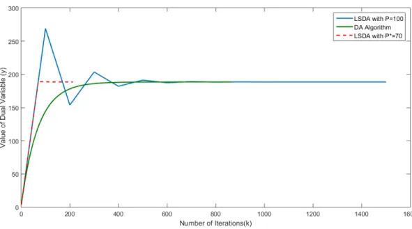
approaches the solution significantly faster than DA algorithm. . . 25 3.8 Convergence of LSDA algorithm with synchronization periods
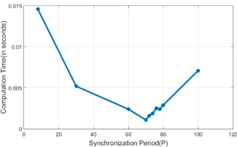
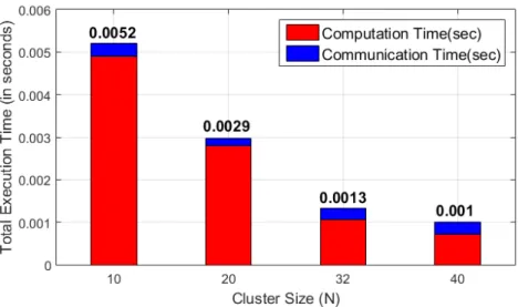
70(op-timal) and 100. It was observed that for synchronization period 100, the convergence is slower than DA algorithm. . . 26 3.9 Variation of computation time and synchronization period . . . 27 3.10 DA algorithm in AWS platform: total execution time i.e., sum of
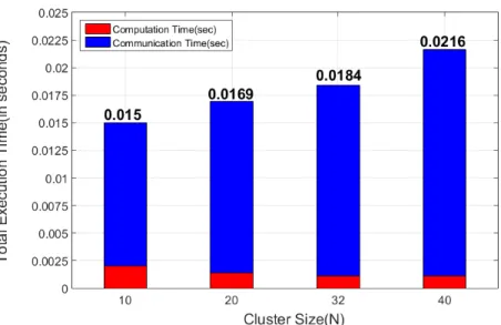
computation time and communication time vs cluster size. . . 28 3.11 LSDA Algorithm in AWS platform: total execution time i.e., sum of
computation time and communication time vs cluster size. . . 28 3.12 Variation of computation time with cluster size (N) and
synchroniza-tion period (P) . . . 29 3.13 DA algorithm in HPC platform: total execution time i.e., sum of
3.14 LSDA Algorithm in HPC platform: total execution time i.e., sum of
computation time and communication time vs cluster size. . . 31
3.15 Speedup(AWS) of overall execution time of LSDA with respect to DA algorithm. . . 32
3.16 Speedup(HPC cluster) of overall execution time of LSDA with respect to DA algorithm. . . 32
4.1 Illustration of SVM classifier. . . 35
4.2 Illustration of generic classifiers. . . 35
4.3 Illustration of soft margin SVM. . . 38
4.4 QR-SVM technique on L2-SVM transforms a 6×6 dense and non-separable coefficient matrix into a sparse block diagonal matrix, where, the first 2 × 2 block is full rank and the second 4× 4 block is a diagonal submatrix. Dense regions are colored. The two blocks in the transformed matrix on the right are outlined in blue. Here,n= 6 and d= 2. . . 45
4.5 QR-SVM framework comprises of two main stages, namely, 1. QR de-composition of the original input matrix ˆXinto Householder reflectors and a matrix R, and 2. Dual Ascent method to solve the QR-SVM problem for obtaining the normalwto the hyperplane and identifying set of support vectors. . . 47
4.6 QR-SVM scales linearly with number of instances, n in the dataset. A synthetic dataset with fixed dimensionality,d=18 and increasing n was used to test scalability with number of instances. . . 54
4.7 QR-SVM scales quadratically with dimensionality, d of the dataset. A synthetic dataset with fixed number of instances, n=100,000 and increasing d was used to test scalability with dimensionality. . . 54
4.8 Comparision of performance of QR-SVM and LIBLINEAR with di-mensionality. A synthetic dataset with number of instances fixed at 100,000 and varying dimensionality was used to make this compari-sion. QR-SVM outperforms LIBLINEAR till a dimensionality of 700. 55 4.9 Convergence of QR-SVM for HIGGS dataset: using QR-SVM we con-verge to a reasonable value of the optimal cost within 20 iterations. . 55
4.10 Convergence rates of QR-SVM vs LIBLINEAR. QR-SVM converges relatively faster compared to LIBLINEAR. Here, we illustrate for 250 iterations. LIBLINEAR was not able to converge to the optimal cost value in 1500 iterations while QR-SVM converged to the optimum in 80 iterations. . . 56 A.1 Sparsity map of QR decomposition. . . 68 A.2 Householder transformation on a vector in 2D space. . . 69
LIST OF TABLES
TABLE Page
4.1 QR-SVM training time details . . . 56 4.2 Comparison - QR-SVM and LIBLINEAR . . . 57
1. INTRODUCTION
With the advancement in computing systems, several industries and organiza-tions started to invest heavily in data analytics to develop data-driven soluorganiza-tions to problems such as expenditure balancing, real-time solutions to customer problems, business intelligence and also to explore new horizons to expand businesses. Ma-chine learning has also interleaved itself into other areas of science and engineering. For example, genetic engineers extensively use data analytics for pattern recognition and gene modeling[22]. Computer architecture community is nowadays adopting machine learning techniques for branch prediction[13] and malware detection [15]. Hence, there is a constant need to improve the performance of such data analytic tasks either from an algorithmic perspective or through dedicated computing re-sources.
Large-scale optimization algorithms are the crux of many statistical and machine learning problems. Many of the optimization algorithms used in SVM modeling are iterative in nature. Several researchers target different aspects of the algorithm to improve the performance further. The classic trade off is the per-iteration cost and rate of convergence [11]. Most of the existing algorithms fall at the two extremities of this paradigm. The low per-iteration cost algorithms are used only for developing an approximate yet reasonable model while the fast convergence algorithms which can generate highly accurate models require powerful computing systems to deal with high computation costs. Hence, new algorithms are needed which can both reduce the per-iteration cost as well as have a quick rate of convergence.
A general shift towards dedicated hardware is observed in the recent years to fur-ther improve the performance of the optimization algorithms and fur-thereby providing
real-time solutions to these data-intensive problems [2, 27]. While a majority of them target a particular application, a few like [35] target a generic optimization engine and build a framework for modeling hardware. With the increasing computing power and rise in popularity of the Internet of Things (IoT), embedded data processors on smart devices are the need of the future. Such embedded data processors can be used to obtain meaningful information from the raw data collected by IoT sensor devices. Smart filtering mechanisms [3] are required in such scenarios to remove un-necessary/obvious data and only send important data points to the centralized IoT server. These filters can easily be modeled using embedded data processors. Such requirements reinforce the need for algorithms with low computation costs and good convergence rates based on which dedicated hardware can be built.
The future of computing systems is moving from today’s symmetric multiproces-sors to tightly integrated heterogeneous processor systems and further into exascale computing [19, 31]. The algorithms should, therefore, be adaptable to distribution, decomposition and parallelization with each task solving a subproblem in various multiprocessor architectures. These distributed algorithms rely on synchronization between processors to maintain consensus and this synchronization accounts for the majority of communication overhead in the form of idling across processors. This synchronization overhead in distributed optimization problems can sometimes ac-count for almost 60% of the total execution times[32] and hence, become a bottleneck when scaled to a large number of processors. We present a relaxed synchronization approach to alleviate this communicate bottleneck and thereby improving the per-formance in distributed environments. As this relaxed synchronization methodology is generic and at an algorithmic level, distributed environments ranging from massive supercomputing clusters to small embedded multiprocessors can leverage its benefits. In this thesis, we explore the capabilities of relaxed synchronization in case of
distributed optimization using dual ascent algorithm. This distributed optimization framework will serve as the computing engine to solve an SVM classification problem. Based on the need and the nature of the problem, the distributed optimization framework can be scaled from a single processor to as large as the hardware can support. In case of single processor system, this relaxed synchronization methodology manifests itself as a technique to compute the optimal step size.
The main contributions of this thesis are:
1. Formulation of lazily synchronized dual ascent algorithm(LSDA) for solving a large-scale quadratic programming problem.
2. Experimental validation of the theoretical results to show that the number of it-erations, and thereby execution time, can be significantly reduced using optimal step size for an optimization problem. Experimental results from two environ-ments, 1) cloud cluster on Amazon web services(AWS) and 2) supercomputing cluster courtesy of Texas A&M High-Performance Research Computing, are be presented.
3. A novel QR decomposition approach to model the quadratic programming problem in linear large-scale SVM classifications (QR-SVM) and its solution via LSDA algorithm formulated in step (1).
4. Analytical derivation of optimal step size for solving QR-SVM in a single pro-cessor environment.
5. Comparision of performance and accuracy of the newly proposed QR-SVM with existing state of the art solver using standard, publicly available benchmarks.
2. RELATED WORK
2.1 Lazily Synchronized Dual Ascent
Dual Ascent is a standard approach for solving constrained optimization problem which dates back to 1960s. Recently, due to the advances in computing systems, there is a renewed interest in proximal techniques like dual ascent(DA), alternating direction method of multipliers(ADMM), Dykstra’s alternating projections method and others[9] to solve large distributed optimization problems. Dual Decomposition is a powerful extension of DA algorithm which distributes the optimization problem into sub-problems. These sub-problems take the form of broadcast-gather archi-tecture. Dantzig et.al [14] popularized dual decomposition methods for large-scale linear programming problems. Nedi´c et.al [36] discussed this approach in their recent survey on distributed techniques. Augmented Lagrangian and method of multipli-ers improve the dual ascent algorithm making it more robust to solve optimization problems which are not strictly convex[9]. ADMM is a manifestation of the method of multipliers which has been used in several fields to solve distributed optimization problems including SVM [45]. Goldstein et.al. [23] proposed some extensions and pa-rameter selection techniques to improve the performance of ADMM and Alternating Minimization Algorithms(AMA).
The traditional dual decomposition method of dual ascent does distribute the op-timization problem. However, it requires us to synchronize after every iteration step. Lazily Synchronized Dual Ascent(LSDA) relaxes this constraint by synchronizing at an interval of P, thereby reducing the communication between processor nodes. Our experiments show that we can reduce the communications up to almost 90% when dealing with well-conditioned optimization problems. While the LSDA algorithm is
developed in the spirit of distributed systems, we can extend the same analytical results even for a non-distributed, single processor systems. It can be shown that the analytical derivations in such single processor systems lead to optimal step size selection (analogous to optimal synchronization period in distributed systems) for the optimization problem.
In this thesis, we provide analytical derivation to obtain the optimal synchro-nization period P for the LSDA algorithm and empirically validate these results in a distributed environment with varying cluster sizes.
2.2 QR-SVM Framework
Support Vector Machines(SVM) close to the current form was introduced by Boser, Guyon and Vapnik [7] in 1992. Over the next few years, the model was devel-oped by introducing the kernel trick, loss functions and slack variables to improve the performance and robustness of the classifiers[5]. However, with the growing dataset sizes, the performance of SVM solvers hit a snag. To counter these performance issues, Vapnik [12] suggested a chunking approach to reducing the dataset sizes by purging non-support vector data points from the training sets. Osuna et.al [18] pro-posed operating on subsets individually one at a time, while rest of the data points and their weights are left unchanged. One of the most prominent contributions on algorithmic enhancements for SVMs was the sequential minimization optimization (SMO) by Platt [37] which takes the decomposition method proposed by Osuna to the extreme and optimizes only two points at a time. LIBSVM, which incorporates SMO, is a popular machine learning library targeted mainly for beginners in the field of machine learning [10]. There have been several extensions and hybrids of SMO improving the performance and stability further. One of the prominent modifications widely used was proposed by Keerthi et.al. [30].
Recently, much of the research in this area is targetted towards solving linear SVM classifiers rather than non-linear classifiers. As clearly explained in [44], for large scale SVM problems, training a non-linear classifier is a tedious and time-taking process. It has been observed that for several rich dimensional datasets, the accuracy of linear SVM classifiers is on par with that of non-linear SVM models. Also, training linear classifiers is much faster as it does not involve kernel transformations on the data points. Bottou [8] presented a stochastic gradient descent approach for solving linear SVM. Joachims [28] introduced a cutting plane method for solving large-scale linear SVM problems. SV Mperf is an implementation of this cutting plane technique. Hsieh et.al [25] presented a coordinate decent approach for solving the dual problem of SVM and showed that they outperform other classifiers when dealing with high dimensional datasets. LIBLINEAR [20] is the publicly available library which implements this dual coordinate descent (DCD) method. However, it was found that the dual coordinate descent method is not stable for non-document datasets especially when the number of dimensions is low [11].
In this thesis, we present a novel QR-SVM approach to solving the dual SVM problem targeting problems which cannot be solved using DCD method, i.e., datasets with low dimensionality.
3. LAZILY SYNCHRONIZED DUAL ASCENT*
3.1 Introduction - Dual Ascent
Dual Ascent(DA) is an algorithm to solve linear constrained convex optimization problems. Consider a convex optimization problem
min
x f(x)
subject toAx=b
(3.1)
where x∈Rn is the primal variable which minimizes the objective functionf while satisfying the constraint Ax=b where A ∈ Rm×n and b ∈
Rn. It should be noted that the functionf :Rn →
Ris a strict convex function and hence any local minimum is in fact a global minimum.
The Lagrangian for problem (3.1) is given as
L(x,y) =f(x) +yT(Ax−b) (3.2)
where y ∈ Rm is the Lagrangian or dual variable. The size of dual variable y is dependent on the number of constraints in the original optimization problem, m.
Solving the optimization problem in (3.1) is equivalent to solving its dual problem as given below: max y inf x L(x,y) (3.3) Ify∗is the optimal solution to the dual problem (3.3) and assuming strong duality
*Part of the content in this chapter is reprinted with permission from “A relaxed
synchroniza-tion approach for solving parallel quadratic programming problems with guaranteed convergence” by Kooktae Lee, Raktim Bhattacharya, Jyotikrishna Dass, V N S Prithvi Sakuru, and Rabi N
holds, the optimal primal variable x∗ can be obtained by solving
x∗ =argmin
x L(x,y
∗ )
Finally, to solve the optimization problem for x∗ and y∗ the following gradient steps can be used:
xk+1 = arg min
x L(x,y
k) yk+1 =yk+ηk(Axk+1−b)
(3.4)
whereηk >0 is the step size for the kth iteration. These update steps are
contin-ued till the dual variable yconverges to an -accurate solution i.e., |yk+1−yk| ≤ . Notice that the optimization problem considered is an equality constrained problem. By ensuring each of the dual variableyi is greater than or equal to 0, the dual ascent algorithm can be extended to inequality constrained (Ax ≤ b) optimization prob-lem i.e., the update steps for an inequality constrained optimization probprob-lem are as follows: xk+1 =argmin x L(x,y k) yki+1 =max(0,yˆki+1) (3.5) where ˆyk+1=yk+ηk(Axk+1−b). 3.1.1 Dual Decomposition
Dual Decomposition is a powerful extension of dual ascent algorithm used to distribute the optimization problem into sub-problems each of which can be solved in parallel. If the convex function f in (3.1) is separable, then the objective of the
minimization problem can be written as
f(x) = X i
fi(xi)
where primal variable x = (x1;x2;...xi;...). Each partitioned sub-vector xi can be updated in parallel without any dependency on other sub-vector partitions.
The coefficient matrix in the constraint equation is trivially separable and can be written as
A = [A1, A2, ...Ai, ...]
Hence, the update steps in case of dual decomposition can be formulated as: xki+1 =argmin xi Li(xi,yk) yk+1 =yk+ N X i=1 ηikAixki+1− b N (3.6)
where N is the number of sub-vector partitions of variable x. As clearly observed in (3.8), each of the x update can be done in parallel by independent worker nodes. However, for dual variable update, the components of xfrom each individual worker nodes should be gathered. The newly updated value of dual variable should then again be broadcasted to the worker nodes for the next iteration. Hence, dual decom-position clearly follows a broadcast-gather architecture in distributed environments.
3.1.2 Quadratic Programming Using Dual Ascent
This section explores a specific example of dual ascent; solving a quadratic pro-gramming problem using dual ascent. A quadratic propro-gramming (QP) problem is an optimization problem which minimizes or maximizes a quadratic objective function subject to linear constraints. A standard QP problem can be formulated as
Figure 3.1: Process distribution of a separable QP problem. min x 1 2x TQx+cTx subject toAx=b (3.7)
The update steps for solving the QP problem (3.7) using dual ascent are
xk+1 =argmin
xi
Li(xi,yk) = −Q−1(ATyk+c)
yk+1 =yk+ηk(Axk+1−b)
To apply dual decomposition, the objective function f should be separable. The objective function in (3.7) is separable if the Q matrix is block diagonal. A block diagonal matrix Q would imply that the components of x pertaining to one block are independent of the components in the other block and hence can be solved in
parallel. The update steps in case of a block diagonal Qmatrix are xki+1 =−Q−i 1(ATi yk+ci) yk+1 =yk+h N X i=1 ηi Aixki+1− b N i (3.8)
whereQi is the ith block in the block diagonal matrixQ. Figure 3.1 pictorially shows this distribution.
3.2 Proposed - Lazily Synchronized Dual Ascent
This section details the proposed lazy synchronization technique and provides the analytical analysis of the algorithm for Quadratic Programming (QP) problems. From equations in (3.8), it is observed that the update equation of y can be in-terpreted as part of a discrete-time system and the convergence of the iterations is dependent on the stability of this system. Such analogy between discrete-time systems and iterative algorithms can be observed in Lee et.al. [33].
In a typical implementation of equation (3.8), x-updates are computed in parallel and then synchronized to calculate the y-update. This sequence is carried out for every iteration. Lazy synchronization strategy relaxes this requirement and the x-updates are synchronized only at certain time period P. Hence, the update equation of the dual variable y can now be written as
yk+1 =yk+h N X i=1 ηi AixtPi +1− b N i (3.9) where tP ≤k <(t+ 1)P, t∈N0
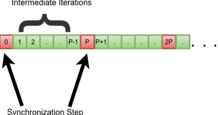
Figure 3.2: Distribution of iterations of dual ascent algorithm with a synchronization period P
steps as shown in figure 3.2. So, for a given intermediate iteration i.e., tP ≤ k <
(t+ 1)P, yupdate is carried out with the most recently updated values ofxi,xtPi +1. On reaching the next synchronization step, (t+ 1)P, each individualxi is computed and communicated across nodes, and the updated values i.e., x(it+1)P+1 are now used for the subsequent y updates during the itermediate iterations.
3.2.1 Stopping Criteria of LSDA
The algorithm is bound to terminate when change in the dual variable is small defined by
||yk+1−yk||2 ≤
where is the stopping threshold. From equation (3.9), it can be observed that during intermediate iterations that the change in the dual variable is a constant determined by xtP+1. Hence, the stopping criterion of the LSDA algorithm can be
redefined as N X i=1 ηi AixtPi +1− b N 2 ≤ (3.10)
Note that the convergence is bound to occur only on the synchronization steps when xtP+1 changes to x(t+1)P+1, as x is the only variable in equation (3.10). The
error during the intermediate iterations is fixed and same as that of the error at the last synchronization step.
3.2.2 Stability of LSDA
Stability of LSDA determines the algorithms ability to converge to the optimal solution. Increasing the synchronization period, P decreases the amount of commu-nication between iterations. However, if the period P crosses a certain threshold, then dual variable y will start to diverge and the algorithm will fail to converge to the optimum value. The below lemma 1 establishes the stability of LSDA algorithm. Lemma 1 [32] The dual variable y update for LSDA algorithm is stable if and only if ρI−P N X i=1 ηi(AiQ−i 1A T i ) <1 (3.11)
where ρ(·) represents the spectral radius.
Proof: Consider a discrete-time dynamic system of the form yk+1 = Ayk +b, where A is a time-invariant matrix and b is a constant vector. The stability of such a system is determined by the spectral radius of the matrix A. yk converges to y∗ if and only if the spectral radius of A is less than 1 i.e., ρ(A)<1.
From equation (3.8), xtPi +1 =−Q−i 1(AT
i ytPi +ci). Subsituting xtPi +1 in equation (3.9), the dual variable update equation can be written as
yk+1 =yk+ N X i=1 ηi −AiQ−i 1(A T i y tP +c i)− b N where tP ≤k <(t+ 1)P
Towards the end of the iterations in a synchronization period i.e. k = (t+1)P−1, the y update can be analytically written as
y(t+1)P =ytP +P N X i=1 ηi −AiQ−i 1(A T i y tP +c i)− b N (3.12) =ytP +P N X i=1 ηi −AiQ−i 1A T i y tP+P N X i=1 ηi −AiQ−i 1ci− b N =ytP −P N X i=1 ηi AiQ−i 1A T i ytP −P N X i=1 ηi AiQ−i 1ci+ b N ⇒y(t+1)P =I−P N X i=1 ηi(AiQ−i 1A T i ) ytP −P N X i=1 ηi AiQ−i 1ci+ b N (3.13) From the above equation (3.13), the stability of LSDA algorithm can be deter-mined as ρI−P N X i=1 ηi(AiQ−i 1A T i ) <1 3.2.3 Convergence of LSDA
While the stability analysis in section 3.2.2 ensures convergence of LSDA algo-rithm, convergence to the same optimal solution as that of the conventional dual ascent algorithm can be proved through the following proposition.
Proposition 1 [32] Given a QP problem and ensuring the stability of LSDA as defined in lemma 1 for that QP problem, the dual variable y of LSDA algorithm
converges to the same optimal value as that of conventional DA algorithm.
Proof: As the stability condition for LSDA algorithm is satisfied, it is bound to converge to a certain value of dual variable yas t→ ∞
y∗ = lim t→∞y (t+1)P From equation (3.13) ⇒y∗ =I−P N X i=1 ηi(AiQ−i 1A T i ) y∗−P N X i=1 ηi AiQ−i1ci + b N ⇒P XN i=1 ηi(AiQ−i1A T i ) y∗ =−P N X i=1 ηi AiQ−i 1ci+ b N ⇒ N X i=1 ηi(AiQ−i 1A T i ) y∗ =− N X i=1 ηi AiQ−i 1ci+ b N ⇒y∗ =− N X i=1 ηi(AiQ−i 1A T i ) −1XN i=1 ηi AiQ−i 1ci+ b N (3.14)
A similar analysis of dual update equation of conventional DA algorithm shown in (3.8) would result in the same optimal value of dual variabley∗. Hence, it can be concluded that both LSDA and conventional DA algorithms converge to the same optimal value of dual variable y∗.
While a direct analytical result of y∗ can directly be obtained from (3.14) itera-tion are often preferred as calculaitera-tion of inverse might be expensive and practically infeasible for large QP problems.
3.2.4 Optimal Synchronization Period
Optimal Synchronization Period,P∗ corresponds to that synchronization period with would minimize the communication between the nodes while also ensuring fast
convergence of the algorithm. Consider the matrix M = PN
i=1ηiAiQ
−1
i ATi . From lemma 1, it has been established that the stability of the LSDA is dependent on the spectral radius of M and that the spectral radius should be less than 1. It follows that, lower the spectral radius of matrix (I−M P), higher is the stability of the LSDA algorithm and hence, the algorithm is bound to converge faster. Hence, the optimal synchronization period of LSDA is that period P∗ where the spectral radius is minimum. It should be noted that the domain of P is the set of Natural numbers i.e., P ∈N and ifP∗ = 1 then the LSDA algorithm behaves similar to the conventional DA algorithm.
Theorem 1 [32] For a given separable QP problem, the optimal synchronization period P∗ for LSDA algorithm is given as
P∗ = max arg min
P∈N max{|1−λ(M)P|,|1− ¯ λ(M)P|} (3.15) where M =PN i=1ηiAiQ −1
i ATi , λ(·) and nλ¯(·) represent the minimum and maximum eigenvalues of the matrix respectively.
Proof: The optimal synchronization periodP∗ corresponds to the minimal spec-tral radius of matrix (I−M P). This can be analytically written as
P∗ = arg min
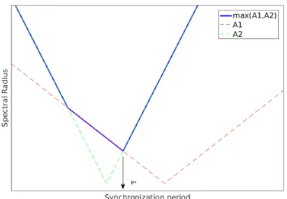
Figure 3.3: Optimal synchronization period, P∗ as derived in equation (3.16). Here,
A1 = |1−λ(M)P| and A2 =|1−λ¯(M)P|.
From the definition of spectral radius,
P∗ = arg min P∈N max v vT(I −M P)v ||v||2 = arg min P∈Nmaxv 1− vT(M P)v ||v||2 = arg min P∈N max v 1− vTMv ||v||2 P
wherevis the eignevector of the matrix (I−M P). Given the symmetric semi-positive definite matrix M, the below expression is valid
λ(M)≤ v TMv ||v||2 ≤λ¯(M) ⇒λ(M)P ≤ v TMv ||v||2 P ≤¯λ(M)P
P∗ = arg min
P∈N max{|1−λ(M)P|,|1− ¯
λ(M)P|} (3.16)
The maximum of the possible synchronization period is chosen in such cases to ensure least amount of communication. Figure 3.3 is a graphical presentation of the expression in (3.16).
3.2.5 Theoretical Speedup of LSDA
To determine the theoretical speedup of LSDA algorithm we use the below defi-nitions
• kDA∗ : the total number of iterations up to termination of Dual Ascent algorithm.
• kLSDA∗ : the total number of iterations up to termination of LSDA algorithm.
• tpDA: computation time per iteration of Dual Ascent algorithm.
• tpLSDA: computation time per iteration of LSDA algorithm.
• tc
DA: communication time per iteration of Dual Ascent algorithm.
• tc
LSDA: communication time per iteration of LSDA algorithm.
• TDA: Total execution time of Dual Ascent algorithm.
• TLSDA: Total execution time of LSDA algorithm.
The total execution time of conventional dual ascent algorithm is given as
TDA =kDA∗ (t p DA+t
c DA)
and the total execution time of LSDA algiorithm is given as
TLSDA =kLSDA∗ tpLSDA+ t c LSDA P∗
We divide the per iteration communication time by the synchronization periodP∗
because out of the total number of iteration we communicate only at time intervals of P∗. Hence, the speedup is given as
Speedup = TDA TLSDA = k ∗ DA(t p DA+tcDA)
k∗LSDAtpLSDA+tcLSDA
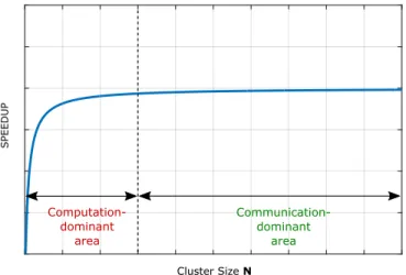
P∗ (3.17) Substituting rk = k∗DA/k ∗ LSDA, rp = tpDA/tpLSDA, rDA = tcDA/t p DA and rLSDA = tc LSDA/t p LSDA in (3.17) Speedup =rkrp 1 +rDA 1 + rLSDA P∗ ! (3.18) From equation (3.18), it can be observed that with an increase in the synchro-nization period, the speedup also increases assuming the ratio of the number of iterations rk is fixed with the change in synchronization period. Cluster size N de-fines the number of subproblems the original QP problem is divided into. With an increase in the cluster size, the amount of computation required on each cluster node decreases while the communication increases as now we need to synchronize between larger number of nodes. Hence, the ratio of communication time to computation time for both DA algorithm (rDA) and LSDA algorithm (rLSDA) increases. But due to the factor P∗, it is observed that the speedup tends to increase with cluster size
N as long as the computation time is dominant over communication time. But at a certain cluster size, communication time dominates over the computation time and the speedup thereafter tends to flatten out. This trend can be observed in figure 3.4.
Computation-dominant area Communication-dominant area Cluster Size N SPEEDU P
Figure 3.4: Theoretical speedup of LSDA when compared with conventional DA algorithm.
3.2.6 LSDA in a Single Processor Environment
The idea of lazy synchronization is presented mainly targeting distributed en-vironments where the cluster sizes are greater than 1. However, the concept of minimum spectral radius for fast convergence can also be applied to dual ascent al-gorithm in single processor environments. From equation (3.12), substitutingN = 1 we get y(t+1)P =ytP +P η1 −A1Q−11(A T 1y tP +c 1)−b (3.19) Redefining Q1 as Q, A1 as A, c1 as c and considering P η1 as ¯η, equation (3.19) is
analogus to a conventional DA update step with a step size of ¯η
y(t+1)P =ytP + ¯η−AQ−1(ATytP +c)−b
By computing the optimal synchronization period as discussed in section 3.2.4 in this setting, we would obtain optimal step size for the dual ascent algorithm in the
form of η∗ =P∗η.
3.3 Experimental Results
The experiments to validate the analytical results of LSDA algorithm were per-formed on two different platforms with varying cluster sizes N = {10,20,32,40}. The QP problem was fixed throughout the experiments. First, the tests were run on Amazon Cloud Compute cluster platform with conventional gigabit interconnect. This platform was close to everyday commodity computers connected with gigabit ethernet connections. The second set of tests were performed in HPC cluster plat-form which supports InfiniBand Communication. Both LSDA and DA algorithms converge to the same solution of the dual variable on termination. Irrespective of cluster size and platform LSDA algorithm consistently outperformed DA algorithm while converging to the same -accurate solution.
3.3.1 Implementation
The LSDA and DA algorithms were implemented in C++11 supported by Ar-madillo(v5.4002) [39] linear algebra library. The Communication across nodes was handled via Message Passing Interface (MPICHv3)[42]. Algorithm 1 shows the pseu-docode for the proposed LSDA algorithm.
The AllReduce method is used for synchronization between the nodes. This AllReduce operation uses the SUM operator to combine multiple sumLocals to compute sumGlobal. AllReduce is a blocking operation which implies all the in-dividual nodes wait till the AllReduce operation is complete, thereby ensuring guaranteed synchronization when invoked. As clear from the pseudocode line 11, termination of LSDA algorithm is only dependant on the sumGlobal value which changes only when the iteration k = tP, where t = 0,1,2,3.... Hence, the LSDA terminates only during a synchronization step (k =tP) and not during intermediate
Algorithm 1 LSDA algorithm 1: function LSDA(Qi,Ai,ci,b,P,,ηi) 2: y ←y0;error ← ∞;k= 0; 3: sumLocal ←¯0;sumGlobal←0;¯ 4: while error > do 5: if k%P == 0 then 6: xi =−Q−i 1(ATi y+ci) 7: sumLocal=ηi(Aixi+Nb)
8: AllReduce(sumLocal, sumGlobal)
9: y=y+sumGlobal
10: error=|sumGlobal|2
11: k+ = 1
iterations (tP < k <(t+ 1)P).
3.3.2 Experimental Setup and Hardware
Synthetically generated random matrices with values uniformly distributed be-tween [-1,1] were used as input datasets for QP problem. The problem specifics are
1. Number of instances, n = 200,000. 2. Step size,η = 0.27.
3. Optimal Synchronization Period, P∗ = 70. 4. Stopping threshold, = 1e-5.
5. Cluster Size, N ={10,20,32,40}
Cluster sizes were chosen such that the data can be evenly distributed among the cluster nodes i.e., factors of n.
The experiments were run on two different hardware platforms − 1) Amazon Cloud Platform and 2) HPC Cluster Platform.
3.3.2.1 Amazon Cloud Platform
40 node Amazon Web Services(AWS) Elastic Cloud Compute(EC2) instances were used[26]. The EC2 instances were created using the t2.micro configuration with each instance backed by Intel Xeon processors with a clock speed of 3.33GHz. Each instance was supported by 8GB disk memory with 1GB main memory. The instances were connected using gigabit ethernet and originated from the same data center in Oregon. This hardware platform was aimed to mimic the commodity computers connected using basic LAN.
3.3.2.2 HPC Cluster
EOS supercomputing cluster provided by Texas A&M High Performance Research Computing consists of 8-core 64-bit Nehalem processor. The nodes were connected by InfiniBand (IB) interconnect with a duplex speed of up to 5 GiB/s. Intel MPI was used in this case rather than MPICH as it supports IB interconnect. Though the EOS cluster offers computer nodes up to 314, we restricted the experiments to 40 nodes to ensure a fair comparison with AWS platform. Figure 3.5 shows a block schematic of the EOS cluster.
3.3.3 Results and Discussion
Results include analysis of 1) Synchronization Period, 2) Computation Time, 3) Communication Time and 4) Speedup with varying cluster sizes to compare the performance of LSDA algorithm against DA algorithm.
3.3.3.1 Synchronization Period
The number of iterations skipped between two successive inter-node communica-tion is defined by the synchronizacommunica-tion period P.
Figure 3.5: Blo ck sc hematic of EOS cluster. Source: T exas A&M Hig h-P erformance Researc h Computing (h ttp://hprc.ta m u.edu/)
Figure 3.6: Variation of number of iterations to converge with synchronization period.
Figure 3.7: Convergence of LSDA algorithm and DA algorithm. LSDA algorithm approaches the solution significantly faster than DA algorithm.
Figure 3.8: Convergence of LSDA algorithm with synchronization periods 70(opti-mal) and 100. It was observed that for synchronization period 100, the convergence is slower than DA algorithm.
It was observed that synchronization period was the only factor effecting the number of iterations when stopping threshold () and step size (η) are fixed. The cluster size should have no effect on the termination of LSDA algorithm as expected. This is becausesumGlobal in Algorithm 1 would remain the same irrespective of the number of cluster nodes. Figure 3.6 shows the variation of the number of iterations to converge with cluster size. This is close to the theoretical result shown in figure 3.3. It is observed that for the synthetic dataset considered the optimal Synchronization period is 70. Also, from theoretical derivation, it was found that the matrix M for this dataset (from section 3.2.4) is a scalar value of 0.0143 which leads to optimal synchronization period to be 70. This validates the theoretical results on optimal synchronization period.
Figure 3.9: Variation of computation time and synchronization period
DA algorithm. The algorithm converges to the optimal solution y∗ in 211 iterations while DA took 868 iterations. This behavior validates that LSDA algorithm is both numerically stable and accurate even with the relaxed synchronizations. Figure 3.8 shows that for synchronization periods much larger than the optimal period, the conventional DA algorithm might perform better than LSDA algorithm.
3.3.3.2 Computation Time
The time spent in calculations other than theAllReduce step in Algorithm 1 is considered as Computation time.
Variation with Synchronization Period: For a given cluster size and chang-ing synchronization period, we observe that computation time follows the similar trend as that of the number of iterations. This is evident from figures 3.9 and 3.6. The minimum computation time occurs at a synchronization period of 70 (optimal value). The variation of computation time with cluster size and synchronization period can be seen in figure 3.12.
Figure 3.10: DA algorithm in AWS platform: total execution time i.e., sum of com-putation time and communication time vs cluster size.
Figure 3.11: LSDA Algorithm in AWS platform: total execution time i.e., sum of computation time and communication time vs cluster size.
Figure 3.12: V ariation of computation tim e with cluster size (N) and sync hronization p er io d (P)
Variation with Cluster Size: Given that the optimal synchronization period
P is 70, the computation time was analyzed with changing cluster sizes at this value of P. As the cluster size increases, the data load on each cluster minimizes and hence the computation time decreases as cluster size increases. This is a trend which can be seen both in LSDA and DA algorithm as shown in 3.10 and 3.11. When compared with the computation time of DA algorithm, we see a significant decrease. This decrease is mainly attributed to reduced number of iterations. This trend is observed irrespective of the platform used as evident from figures 3.13 and 3.14.
3.3.3.3 Communication Time
The time spent in the inter-node communication, i.e. synchronization in case of LSDA and DA algorithms, is defined as Communication Time.
Figure 3.11 shows communication time of LSDA algorithm with increasing clus-ter size N. However, this trend is not strictly followed due to other traffic and noise on the network which is non-deterministic. In HPC platform, we see that the com-munication time is closer to the expected behavior yet not strictly followed. Figures 3.13 and 3.14 show the communication time in HPC cluster platform.
3.3.3.4 Speedup
Figure 3.15 shows the speedup of execution time which is the sum of computation time and communication time achieved by LSDA algorithm over the DA algorithm. We see that a speedup of around 160×(±12.5) is obtained in case of AWS platform. It should be noted that the speedup is almost constant. Such flattened speedup is the theoretically expected trend as observed in section 3.2.5. The flattening of speedup shows that the cluster sizes selected fell in the communication dominant region. In the case of HPC cluster platform, we observe a stark difference as the computation time dominates over the communication time. This domination of the computation
Figure 3.13: DA algorithm in HPC platform: total execution time i.e., sum of com-putation time and communication time vs cluster size.
Figure 3.14: LSDA Algorithm in HPC platform: total execution time i.e., sum of computation time and communication time vs cluster size.
Figure 3.15: Speedup(AWS) of overall execution time of LSDA with respect to DA algorithm.
Figure 3.16: Speedup(HPC cluster) of overall execution time of LSDA with respect to DA algorithm.
time over the communication time is mainly due to the high performance computing flavored InfiniBand(IB) interconnect used in the HPC platform for communication. Figure 3.16 shows the speedup of LSDA algorithm over DA algorithm solving the same problem as that of AWS cluster in an HPC cluster platform. The speedup tends to increase as we fall in the computation dominant region, evident from figure 3.14. This validates our theoretical results on speedup in section 3.2.5.
3.4 Conclusion
In this chapter, we introduced a lazy synchronization technique to solve quadratic programming problem using dual ascent algorithm. Analytical proofs show that this approach ensures faster convergence of the optimization problem than conventional DA algorithm. We both analytically and empirically prove that communication time is greatly reduced using LSDA algorithm. For the experimental data used, we show that empirically communication time is reduced by almost 99% as we synchronize only three times in case of LSDA algorithm rather than 868 times in case of DA algorithm. With the optimal synchronization period, we also reduce the total number of iteration to converge to an -accurate solution. In addition, we also prove both analytically and empirically that irrespective of the cluster size we would still attain a constant speedup.
4. QR - SVM
4.1 Introduction - Support Vector Machines
Support Vector Machines (SVMs) is a popular machine learning classification technique first introduced by Boser, Guyon and Vapnik [7]. The primary objective of an SVM model is to maximize the separation margin between the data points of different classes thereby forming the best possible separation hyperplane. Hence,
d-dimensional data points are separated by a (d−1)-dimensional hyperplane. This method is a form of supervised learning where the class label of each of the data points is available before the training phase begins. The original SVM was designed for a binary classification problem. To solve a multivariate (more than 2 classes) classifi-cation problem two commonly used strategies are one-versus-one and one-versus-all [6, 17] techniques where multiple SVM models are trained either sequentially or in parallel.
Though SVM is commonly used to solve classification problems, the idea, i.e. optimal margin, is not restricted to supervised classifiers alone. There are several variations like support vector clustering [4], support vector regression [16] and one-class SVM [40] which solve clustering, regression modelling and anomaly detection problems respectively.
Figure 4.1 illustrate a simple SVM model of 2-dimensional data where H1 denotes the 1-dimensional maximal margin hyperplane classifying the data. In figure 4.2, hyperplanes H2 and H3 also classify the data; however, they are not the best possible solution with least generalization error. Generalization error in a supervised learning context indicates the accuracy of the model in predicting the results of unseen data i.e., out-of-sample error [1].
Figure 4.1: Illustration of SVM classifier.
The advantages of using SVM as a classification technique apart from the math-ematical simplicity are:
1. Low generalization error is observed as the model tries to find the maximum separation margin. This also accounts for robust results as compared against other classifiers.
2. SVM models can easily handle non-linear data spread using the kernel trick. 3. The support vectors (points which lie on the boundary and determine the
hy-perplane) can be used to differentiate between “interesting” and “non-interesting” points. These support vectors essentially carry most of the information in the dataset and can be used in incremental learning [41].
4.1.1 Mathematical Formulation
Given n training data points in d-dimensional space belonging to two classes
{−1,+1}i.e., given data points (x1, y1),(x2, y2). . .(xi, yi). . .(xn, yn) where eachxi ∈ Rd and yi ∈ {−1,1}.The objective is to find a vector w and a bias b such that
wTx+b= 0 (4.1)
is the maximal margin hyperplane.
The valueswand bare normalized such that the support vectors (data points on the boundary) satisfy the equation
|wTx+b|= 1 (4.2)
The modulus in equation (4.2) is necessary so that the support vectors from both the classes are considered. Given this normalization, the margin between the
hyperplane in (4.1) and support vectors reduces to 1
||w||2 2
. Hence, the SVM can now be formulated as a maximization problem:
max w 1 ||w||2 2 subject to yi(wTxi+b)≥1 forn = 1,2, ...n
The above quadratic optimization can be re-written in a more standard mini-mization problem as min w 1 2w Tw (4.3) subject to yi(wTxi+b)≥1 forn = 1,2, ...n
The biasb which is typically associated with the hyperplane can be induced into the vector w by adding an additional dimensionality to the input data pointxi
xi ←[xi; 1] =⇒ w←[w;b]
Eq (4.3) is often referred to as hard margin SVM where the data points are linearly separable in the d-dimensional space. However, this is not the case in most of the real-world classification problems. Hence, hinge loss is introduced into the objective function to penalize the misclassifications. Such objective functions are called soft margin SVM. In the case of hard margin SVM (eq (4.3)), there are no misclassifications to begin with, and hence, no loss function is needed.
A soft margin SVM problem is now an unconstrained minimization problem given as
Figure 4.3: Illustration of soft margin SVM. min w 1 2||w|| 2 2+C n X i=1 ξi(w;xi;yi) (4.4) where ξi(w;xi;yi) represents the loss function associated with the optimization problem and C represents the penalty parameter i.e., how much is a data point penalized for a classification error. Hence, when the penalty parameter C is increased the classifier becomes more strict. Figure 4.3 illustrates the use of soft margin SVM. For a low penalty parameter C, the classifier considers the best margin solution even though there are some data points within the margin. If the penalty parameter was high, the SVM model would not have allowed such points within the margin.
The common loss functions(ξi) used in SVM training are l1-loss(L1-SVM) or l2
l1-loss:
max(0,1−yiwTxi)
l2-loss:
max(0,1−yiwTxi)2 The dual form of optimization problem in (4.4) is
min α 1 2α TZˆα+eTα subject to L≤αi ≤U (4.5)
where ˆZ =Z +D, e is a vector with of negative ones, L is the lower bound of the dual variable and U is the upper bound. Zij =yiyjk(xi,xj) where k represents the kernel function. For linear-SVM, the kernel function k is the dot product of the vectors xi and xj. Diagonal matrix D, lower bound L and upper bound U are dependent of the type of loss function associated with the SVM problem. In case of L1-SVM, D = 0n, L = 0 and U = C while for L2-SVM, D =diag(1/2C)n, L = 0 and U =∞.
The dual form in (4.5) might not be as intuitive as the primal SVM. However, there are several advantages of solving the dual form of SVM over the primal SVM. The dual variableαdenotes the hidden weight of each data point in determining the classifier. If αi is zero, it indicates that the data point xi is towards the interior and away from the margin and if αi is greater than zero, it shows that xi is a support vector and is either on or close to the margin. As explained earlier, these support vectors are useful in decomposition algorithms [43, 24], incremental learning [38, 41]. Another reason for solving the dual problem is to leverage the kernel trick for
non-linear classifiers. SVM is essentially a linear classifier. If the data is not linearly separable, then its mapped to a higher dimensional space where it can be linearly separable and then an SVM model is trained in that high dimensional space. It is not easy to transform data to higher dimensional space and sometimes there can even be infinite number of dimensions. Using the kernel trick, a kernel function k
can be found, such that
k(xi,yi) =hϕ(xi), ϕ(xj)i
where h·,·i represents the inner product and ϕ is the transformation to higher dimensional space ϕ : Rd →
RD. Hence, even without explicit knowledge about ϕ a non-linear classifier can still be trained by using the function k on the original set of data points X in the d dimensional space. Though kernel trick is very useful, for large scale datasets calculating the SVM problem turns computationally infeasible. Hence, we prefer either solving a linear SVM problem in such cases.
4.2 Linear SVM
Linear SVM involves finding the maximal margin hyperplane in the original input data space. The kernel function in the dual form of linear SVM in (4.5) takes the form
k(xi,xj) =hxi,xji
We can rewrite equation (4.5) specific to linear SVM forl1-loss and l2-loss as
l1-loss:
min α
1 2α
Tdiag(y)XXTdiag(y)Tα+eTα
l2-loss:
min α
1 2α
Tdiag(y)XXTdiag(y)Tα+1 2α T 1 2CIn α+eTα subject to 0≤αi ≤ ∞ where X = [xT
1;xT2;xT3...xTn], y = {yi ∈ {−1,1}|i = 1...n} and C is the penalty parameter. Substituting ˆX =diag(y)X,
l1-loss: min α 1 2α TXˆXˆTα+eTα (4.6) subject to −In In α≤C 0n 1n l2-loss: min α 1 2α Tˆ XXˆTα+ 1 2α T 1 2CIn α+eTα (4.7) subject to −Inα≤0n
L2-SVM provides a simpler constraint formulation which specifies eachαi corre-sponding to each dataxi must be non-negative. Moreover, the optimization problem in L2-SVM is strongly convex and smooth when compared to L1-SVM, which makes it easier to solve. For these specific reasons we elaborate proposed QR-SVM mainly for L2-SVM, however, the similar methodology can be extended to L1-SVM as well.
4.2.1 Challenges
Matrices X and ˆX are based on the input of SVM classification problem. The dimension of these matrices is (n ×d) where n is the number of input instances and d is the dimensionality of each data point. In a majority of SVM classification problems, the number of instances is much larger than the dimensionality of a data point, i.e. d n. The ˆXXˆT in equations (4.6) and (4.7) is a dense (n ×n) matrix which is tightly coupled and hence can’t be decomposed into independent sub-problems of smaller size trivially. Working on the whole (n×n) data matrix not only leads to high computational complexities but also loading this O(n2) matrix to
memory is practically infeasible. Also, the quadratic coefficient matrix ˆXXˆT is also rank deficient and hence non-invertible. This makes the dual ascent algorithm highly unstable. To address the above issues, we propose QR-SVM framework comprising of a) QR decomposition technique to efficiently transform the dense coefficient matrix into a sparse form and b) dual ascent method to solve the above optimization problem relatively faster than the state of the art solver.
4.3 Proposed QR-SVM
Some basic preliminary concepts of QR decomposition and various algorithms used to for this decomposition are detailed in appendix A. In this section we first present the motivation for using QR decomposition in Linear SVM, followed by the formulation and benefits of proposed QR-SVM framework for L2-SVM.
4.3.1 Motivation
In a majority of SVM classification problems, the number of instances is much larger than the dimensionality of a data point, i.e. dn. For such SVM problems, the input data setX and the corresponding ˆX are tall skinny matrices. On applying
QR decomposition on ˆX we get
ˆ
Xn×d=Qn×nRn×d
TheRmatrix from QR decomposition, is an upper triangular matrix of sizen×d. The maximum number of possible non-zero elements in this R matrix is d(d+ 1)/2 making it highly sparse when compared to the original matrix ˆX with a maximum of
ndnon-zero elements asdn. So, if we transform the vectorα(equations (4.6) and (4.7)) from the original vector space of the SVM problem to a vector space with basis defined by the orthogonal matrix Q, i.e. αˆ =QTα, we will be dealing with a much smaller data matrix in terms of R. This transformation of vector spaces will thereby sparsify the computations involved in solving the transformed SVM problem. As the data size reduction is dependent on the ratio of d : n, tall-skinny SVM problems yield high computation benefits from this QR decomposition approach.
4.3.2 QR-SVM Formulation for L2-SVM
QR decomposition on a TS-dense ˆX factorizes it into two matrices, namely, Q
and R i.e., ˆX = QR. Here, Q is an orthogonal matrix of size n×n and R is a upper triangular matrix of size n×d. The quadratic programming (QP) problem in equation (4.7) now becomes
1 2α Tˆ XXˆT α+1 2α T 1 2CIn α+eTα (4.8) = 1 2α TQRRTQTα+ 1 2α T 1 2CIn α+eTα = 1 2(α TQ)RRT(QTα) + 1 2α T 1 2CIn α+eTα
On substituting QTα= ˆα, cost function of L2-SVM QP problem formulates to 1 2αˆ T RRTαˆ +1 2αˆ T QT 1 2CIn Qαˆ + (QTe)Tαˆ (4.9) subject to −Qαˆ ≤0n
Defining ˆe=QTe and using QTQ=I n, 1 2αˆ T RRT + 1 2CIn ˆ α+ (ˆe)Tαˆ (4.10) subject to −Qαˆ ≤0n
The QP problem in (4.10) can be interpreted as a combination of two QP problems where the first QP problem deals with the first d components of the vector αˆ and the second QP problem targets the next n−d components of the vectorαˆ.
4.3.3 Benefits of QR-SVM
From (4.10), it can be observed that by transforming the basis of αto αhat, we were able to move the problem to a vector space where the
In equation (4.10), RRT is a symmetric sparse matrix of size n where the first
d×d submatrix is dense while rest of the elements in the matrix are all zeros. In other words, coefficient matrix of the quadratic term in equation (4.10) is a block diagonal matrix comprising of two diagonal blocks: 1) a d×d symmetric and dense submatrix, (RRT)
d+(1/2C)Idand 2) a diagonal submatrix (1/2C)In−d. The benefits of the proposed QR-SVM formulation are listed below.
1. Sparsity: We have transformed a dense n ×n quadratic coefficient matrix ˆ
XXˆT + (1/2C)In in equation (4.8) to a sparse matrix as in equation (4.10) which consists of a small dense d×d block, as illustrated in Figure 4.4. The
Figure 4.4: QR-SVM technique on L2-SVM transforms a 6 × 6 dense and non-separable coefficient matrix into a sparse block diagonal matrix, where, the first 2×2 block is full rank and the second 4×4 block is a diagonal submatrix. Dense regions are colored. The two blocks in the transformed matrix on the right are outlined in blue. Here, n = 6 andd= 2.
sparse coefficient matrix in the proposed QR-SVM consumes (d2 + 1)/(n2) fraction of the memory assigned to the original dense coefficient matrix.
2. Separability: We have also rendered the aforementioned non-separable quadratic coefficient matrix into a block separable form by using the proposed QR-SVM formulation. One can exploit this separability to independently solve the two sub-problems in parallel at each iteration dual ascent algorithm.
3. Invertibility: On applying QR-SVM, thelow-rank quadratic coeffcient matrix becomes block-separable where the two sub-blocks are now invertible. The first block (RRT)
d+ (1/2C)Id isfull-rank in d and the second block (1/2C)In−d is trivially invertible. The invertibility of the quadratic coefficient matrix makes the dual-ascent algorithm stable by allowing the computation of the minimiza-tion step in equation (4.12).
The proposed QR-SVM formulation can be implemented without any additional memory compared to the original problem in equation (4.8). The given input data
ˆ
ma-trix R, which together occupy the same nd− memory space as ˆX. In addition, it is observed that one can recover the values of α (to identify corresponding support vectors) from αˆ by simply pre-multiplying αˆ with series of d− Householder reflec-tors with a computational cost of O(nd). This cost is a lot cheaper compared to the O(n2) computational cost incurred if one directly pre-multiplied the matrix Q
instead. Finally, one can efficiently compute the normal w to the linear classifier by directly pre-multiplying RT to αˆ. It is worth noticing that calculation of RTαˆ can be simplified to RTdαˆd i.e. O(d2), given the special structure of matrix R. The QR-SVM process workflow is illustrated in Figure 4.5.
4.4 Optimization Using Dual Ascent
As detailed in chapter 3, Dual Ascent (DA) algorithm can be used to solve Quadratic Programming optimization problems if the quadratic coefficient matrix is invertible. Both the standard SVM problem in (4.8) and QR-SVM in (4.10) are QP problems. However, it is not possible to solve the standard SVM problem ((4.8)) directly as quadratic coefficient matrix ˆXXˆT + (1/2C)I
n is rank deficient and not invertible. In case of QR-SVM, the quadratic coefficient matrix in QR-SVM is in-vertible and hence can be solved by LSDA algorithm. The Lagrangian L of QP problem in equation (4.10) is written as follows
L( ˆα, β) = 1 2αˆ TRRT + 1 2CIn ˆ α+ (ˆe)Tαˆ+βT(−Qαˆ) (4.11)
where, β ≥0n is the Lagrangian dual variable. Dual ascent update steps for QR-SVM are
4.5: QR-SVM framew ork comp rises of tw o main stages, namely , 1. QR de comp osition of the original input matrix ˆin to H o useholder reflectors and a matrix R, and 2. Dual Asc ent metho d to solv e the QR-SVM proble m for obtaining normal w to the h yp erpla ne and iden tifying set of supp ort v ectors.
Step 1: Minimization of Lagrangian ˆ αk+1 = arg min ˆ α L( ˆα, β k ) =−RRT + 1 2C ×In −1 (−QTβk+ ˆe) (4.12)
Step 2: Dual variable update
βk+1 =βk+η(−Qαˆk+1) (4.13)
whereη >0 is the step size and the superscript k= 0,1,2...is the iteration counter.
β0 is initialized to0
n. To satisfy the inequality constraint on each of the dual variable
βi being non-negative ,βi is replaced with max(0, βi) during every iteration.
While the above update equation (4.12) appear as a single operation to calculate ˆ
α, the actual computation can be distributed among available computation nodes and calculated in parallel independent of each other. Given the block diagonal struc-ture of matrix RRT + 1
2C ×In
, the update equation (4.12) can be split into two major subproblem where subproblem 1 computes the first d elements of αˆ and sub-problem 2 computes the rest of then−delements ofαˆ. Hence, the update equations of the dual ascent algorithm now become
Step 1: Minimization of Lagrangian ˆ αk1+1 =−RRTd + 1 2C ×Id −1 (−QT1βk+ ˆed) ˆ αk2+1 =−2C(−QT2βk+ ˆen−d) (4.14)
Step 2: Dual variable update
where αˆ = [αˆ1;αˆ1] and Q = [Q1;Q2]; Q1 ∈ Rn×d and Q2 ∈ Rn×(n−d). The update equation of αˆ2 in is a simple vector arithematic with can be further distributed
trivially.
4.4.1 Optimal Step Size of Optimization Algorithm
The update steps of the dual ascent algorithm in (4.12) and (4.13) can be opti-mized with respect to step size based on the LSDA formulation based on derivations in Chapter 3, section 3.2.6. The below lemma and corollary will provide the deriva-tion for the optimal step size η∗ used in (4.13).
Lemma 2 (Scaling factor for optimal step size) To ensure the minimum number of iterations involving sequential dual variable update step, the scaling factor P? for optimal step size is obtained by
P? = max arg min
P∈Nmax{|1−λmin(M)P|,|1−λmax(M)P|} (4.16) where, M :=ηRRT + 1
2CIn −1
, η > 0 is step size and λmin(·) and λmax(·) denote the smallest and the largest eigenvalues of the square matrix M, respectively.
On solving equation (4.16), we get the following result.
Corollary 1 For any η >0 , the optimal step size η? can be computed using
η? =P?η, P? ∈N (4.17) where, P? = 1 if 0<¯λ−1 <2 ¯ λ−1 if λ¯−1 ≥2
and λ¯= (λmax(M) +λmin(M))/2
Proof:
On plotting the functionsf1(P) =|1−λmin(M)P| and f2(p) = |1−λmax(M)P|, we can observe that the intersection of the above two functions occurs at point
A(¯λ−1, λ maxλ¯−1−1). max{f1(P), f2(P)}= 1−λmin(M)P if 0< P ≤Ax λmax(M)P −1 if P > Ax ,where, Ax = ¯λ−1
Minimum value of max{f1(P), f2(P)} occurs at point of intersection A. In other
words,
arg min max{f1(P), f2(P)}=Ax. Since, P? ∈
N as per Lemma 2, we must ensure that for 0< Ax <2, optimal scaling factor P? = 1. When A
x ≥ 2, P? is assigned the highest integral value lesser than
Ax, i.e., P? = ¯
λ−1.
This value which is lesser than Ax ensures that the scaling factor is optimum,
P?, and will result in optimal step size, η?, leading to stability and convergence of dual ascent method. It is worth noting that given the special structure of M
comprising of inverse of a block separable sparse matrix (positive semi-definite),
λmin(M) = 2ηC/(1 + 2Cλmax(RRT)) and λmax(M) = 2ηC . For practical values of C in the proposed formulation, λmax(M)λmin(M). Hence, ¯λ−1 ≈1/(ηC) can be used as a good approximation for faster convergence of the dual ascent method.
4.5 Complexity Analysis
The cost of a single iteration of QR-SVM is the combined computation cost of the two update steps defined in equations (4.12) and (4.13). Premultiplying Q (or
QT) to a vector v by using Householder reflectors requires O(nd) operations, where
n is the size of vectorv and d is the number of Householder reflectors [29]. The cost of computing each of (−QTβk) in equation (4.12) and (−Qαˆk+1) in equation (4.13) is O(nd). Given the block diagonal structure of RRT + 21CIn, the computation in equation (4.12) can be split into following:
Subproblem 1: The first d components of ˆαk+1 are computed by solving a
system with the d×d coefficient matrix RRT d +
1
2CId. By computing and storing Cholesky factors of this matrix before starting the iterations, the system can be solved in O(d2) operations. Cholesky factorization of the coefficient matrix is one time calculation that is carried out in the beginning of the dual ascent algorithm at cost of O(d3).
Subproblem 2: Calculation of the remaining (n−d) components of ˆαk+1requires O(n−d)≈O(n) operations since dn.
The overall computation cost of update equation (4.12) is O(nd +d2). Also,
the computation cost of equation (4.13) is trivially O(nd). Combining the above two computation cost for equations (4.12) and (4.13) and including the initial QR decomposition cost, we see that QR-SVM using dual ascent method requiresO(nd2+
knd) operations where k is the number of iterations. The trend is empirically validate in section 4.6.1.2.
4.6 Experiments
The experiments of QR-SVM were performed on a uniprocessor system with LSDA algorithm optimized to work with optimal step size as discussed in sections