issn0092-2102|eissn1526-551X|00|0000|0001 °c0000 INFORMS
Optimizing Highway Transportation at the United
States Postal Service
Anthony Pajunas
US Postal Service, 475 L’Enfant Plaza, SW, Washington D.C., 20260, USA, [email protected], www.usps.gov
Edward J. Matto
IBM Global Business Services, 12902 Federal Systems Park Drive, Fairfax, VA 22033, USA, [email protected], http://www-1.ibm.com/services/us/index.wss
Michael Trick
Tepper School of Business, Carnegie Mellon University, 5000 Forbes Avenue, Pittsburgh, PA 15213, USA, [email protected], http://mat.tepper.cmu.edu/trick
Luis F. Zuluaga
Faculty of Business Administration, University of New Brunswick, PO Box 4400, Fredericton, NB E3B–5A3, CANADA, [email protected], http://www.unbf.ca/business/faculty/luis zuluaga.php
The United States Postal Service (USPS) delivers more than 200 billion items per year. Transporting these items in a timely and cost-efficient way is a key issue if USPS is to meet its service and financial goals. The Highway Corridor Analytic Program (HCAP) is a tool that aids transportation analysts in identifying cost saving opportunities in the USPS surface transportation network. Use of this tool is resulting in millions of dollars of annual savings.
Key words: parcel industry; transportation network; large-scale integer programming; decision support system.
History:
1.
Introduction
The transportation network of the United States Postal Service (USPS) is extremely large and complex, and accordingly the transportation planning process is an important and challenging component of USPS Logistics. The Highway Corridor Analytic Program (HCAP) has recently been developed to assist in the transportation planning process. HCAP is an analytical model intended to aid transportation analysts in identifying cost savings opportunities within the USPS surface transportation network. The HCAP model is designed to solve the Vehicle Routing Problem with Pickups and Deliveries (VRP/PD), utilizing mixed integer programming as the underlying opti-mization engine. The HCAP model also incorporates a graphical user interface to facilitate the modeling process at USPS. HCAP was designed to use existing data sources so the HCAP model can be used for near-term identification of savings opportunities. The HCAP model has been fully developed and tested, and has been deployed to USPS transportation analysts in USPS Head-quarters and in the regional Area offices. Many of the recommendations that have been developed from HCAP model results have been implemented, resulting in annual transportation savings of over $5 million already being realized at USPS during the early stages of HCAP deployment, with additional savings identified and currently under review.
2.
Background
The USPS operates one of the largest and most complex logistics networks in the world, deliver-ing more than 200 billion pieces of mail each year. The USPS surface transportation network is
actually comprised of many different networks, each designed for specific purposes. USPS delivers many different types of mail, including letters, flats (e.g, large envelopes for unfolded documents), parcels, and periodicals. Different types of mail have different characteristics which determine the processing requirements. For example, letters, flats, and parcels all have different sizes, shapes, and weights, resulting in the need for specialized processing operations to accommodate those dif-ferences. USPS also offers several different mail classes, including Priority, First Class (overnight, 2-day, and 3-day), and Standard mail classes. Each mail class has specific service standards that define the overall delivery timeframe for that mail class. To accommodate the wide range of mail type and mail class options available to USPS customers, USPS has established many different transportation networks. For example, the bulk mail network transports bulk mail (e.g, standard parcels, periodicals, and other bulk mail) through Bulk Mail Centers (BMCs); the Surface Transfer Center (STC) network is a transportation network that consolidates mail through STC facilities for purposes of aggregating volumes; inter-plant transportation carries mail among Processing and Distribution Centers (P&DCs); priority mail is often trucked to Priority Mail Processing Cen-ters (PMPCs) for priority mail processing; and time-critical mail (e.g., Express mail and some First Class and Priority mail) is trucked from P&DCs to Air Mail Centers (AMCs) to enter the air transportation network. Each of these transportation networks was designed to serve a par-ticular purpose, but each network does not operate in isolation. Rather, significant overlap and redundancies exist among the various surface transportation networks. For example, inter-P&DC transportation may stop at a BMC en-route between P&DCs, to get bulk mail from the origin P&DC into the bulk mail network. Similarly, STC transportation may additionally stop at P&DCs to pick-up and drop-off inter-P&DC mail along the STC route. These multiple, intertwined trans-portation networks create significant complexities and challenges in USPS transtrans-portation planning. The vast size of the USPS transportation network further complicates the planning process. On an average weekday, for example, USPS may dispatch over 75,000 trips among over 30,000 facilities (including processing facilities, post offices, and other facilities) in the highway transportation net-work. USPS employs a variety of advanced analytical tools and techniques to address the challenges of managing such a large and complex network. The HCAP model was developed to serve as a robust analytical tool to assist in the transportation planning process.
3.
Objectives
The HCAP model was developed to assist USPS in analyzing surface transportation routing and scheduling. The model serves as an analytical tool with which USPS can identify opportunities to reduce surface transportation costs while maintaining on-time delivery. The model is intended to be sufficiently flexible so USPS can apply it to a wide range of components of the USPS transportation network. For example, the HCAP model may be applied to problem sets that include BMCs, STCs, P&DCs, AMCs , and a variety of other transportation applications. The model could also be applied to individual geographic regions of the nation (e.g., all processing facilities in the northeast corridor), or the model could be applied to a single transportation network nationwide (e.g., all BMCs ), provided that the size of the network being considered is suitable for the HCAP model (see Section 4 for details).
Although the HCAP model is designed to be applicable to a wide variety of transportation net-works, there is a standard problem definition that the model is designed to solve. Each problem must be defined by a set of delivery requirements among a set of facilities, and a set of trans-portation resources feasible to transport those deliveries. The HCAP model then optimizes the transportation of the given set of delivery requirements, considering the potential transportation options that can fulfill those delivery requirements. Therefore it is necessary to define, for each problem application, the specific delivery requirements and potential transportation options avail-able. Delivery requirements may include both pickup and delivery requirements among a set of facilities, involving multiple types of mail with various service commitments.
The HCAP model is intended to optimize existing transportation; that is, the model identifies opportunities to modify existing USPS transportation to reduce costs. Although it is not intended as a means to completely self-generate new transportation networks, new transportation options can be considered by the model. For that purpose, it is possible to generate new transportation alternatives using heuristics or operational insights, and incorporate them as potential options that the HCAP model may select when optimizing the network. The solution to the HCAP model will then identify the optimal set of transportation resources based on all options provided as inputs into the model, including existing transportation and any new transportation alternatives provided.
4.
Modeling and Solution Approach
The HCAP model is intended to optimize the use of a wide variety of components of the USPS transportation network. For that purpose, the HCAP model is designed to solve aVehicle Routing Problem with Pickups and Deliveries (VRP/PD) model, a special instance of the more general
Vehicle Routing Problem(VRP) model (see Bodin and Golden (1981) for a classification of various VRP problems). VRP models intend to identify the optimal plan for routing deliveries among facilities. The underlying structure of the model consists of three primary components that can be described as follows:
• Facilities: are the (generally physical) places in the transportation network. In the HCAP model, the locations represent the places at which mail pickups and deliveries occur. For example, these can be P&DC’s, STCs, AMCs and BMCs .
• Deliveries:are the items to be delivered between facilities. In the HCAP model, the deliveries represent the volume of mail that requires transportation from an origin facility to a destination facility in a specific time window (i.e., the time between the moment the mail becomes available at the origin facility and the time the mail is required to be delivered at the destination facility). Each delivery may likely represent a specific mail class, having a certain service standard between the origin and destination (e.g., First Class 3-day mail from New York to San Francisco). Two different types of deliveries are considered in the HCAP model.Splitabledeliveries are those whose associated volume can be divided into different parts for delivery. Conversely,Unsplitabledeliveries are those whose associated volume cannot be divided into different parts for delivery.
• Trips:are the mechanisms (routes) for moving deliveries. In the HCAP model, the trips repre-sent the different means that can be used to transport volume of mail from the origin facility to the destination facility within the required time window. Routes may be direct (from the origin directly to the destination), or multi-stop (stopping at one or more facilities en route from the origin to the destination). Each multi-stop route may pickup and/or deliver mail at any of the facilities along its path. The definition of a trip includes every aspect of the trip: the size (capacity) of the truck, the time at which it arrives and departs at each stop, and the cost of the trip. It is important to note that the trips are defined prior to using HCAP. The set of trips is based on the existing highway transportation network which is primarily contracted from independent contractors.
• Legs:Each trip consists of series of legs between consecutive facilities visited by the trip. Direct trips have only one leg, directly from the origin facility to the destination facility. Multi-stop trips have more than one leg, with each leg connecting two facilities along the route’s path.
Due to the nature of the USPS business, facilities can serve as both origin facilities and destination facilities, and it is therefore possible (and almost always the case) that a single facility may need to both dispatch mail and receive mail. Accordingly, trips may include both pickups and deliveries along the trip, and thus the VRP/PD model is appropriate. Specifically, the HCAP VRP/PD model objective is to assign deliveries to trips such that:
• Assignment Constraints:The total volume of every delivery must be routed on one or (if the delivery is splitable) more of the trips in which the delivery can be routed; that is, the trips that can take the delivery from the delivery’s origin facility to the delivery’s destination facility during the delivery’s time window.
• Capacity Constraints:For every leg of every trip, the total volume associated with the deliveries routed through a trip leg must be less than or equal to the leg’s capacity; that is, the maximum volume that can be routed. In the HCAP model, the legs of a single trip are allowed to have different capacities. This allows the USPS to take into account in the model, the fact that, by choice, some volume of mail (not included as deliveries in the model) will be routed through some trip legs included in the model. For example, in a model of the southwest area, the modeler may desire to consider any excess capacity on trucks that start in the eastern area and pass through the southwest en-route to California. Mail volumes that originated in the eastern area should not be represented as deliveries within the model because they are outside the model scope (since this example is a southwest area model), but the excess capacity of trucks entering the southwest area could be modeled by using the capacity constraints at the leg level, to reflect that some of the capacity must carry the mail volumes that originate in the eastern area and are destined for various stops along the trip to California.
• Minimal Cost:The total cost of routing the deliveries on the available trips is minimized over all the feasible assignments of deliveries to trips; that is, that satisfy both the assignment and capacity constraints. This cost includes the fixed cost incurred for the use of any trip, and the variable cost incurred for routing the volume of the deliveries on particular legs of the trips. The HCAP VRP/PD model can be mathematically formulated (see Appendix for details) as a
Mixed Integer Program (cf. Nemhauser and Wolsey (1988)). In this model, the key decisions to be made are whether to use or not use each trip, and how much of each delivery is to be placed on each accepted trip. This differs from many vehicle routing applications where the trips are not pre-defined. In such cases, models need to combine legs to create trips, which is a much more complicated process. The HCAP integer program is much closer to a facility location model (see, for instance, Drezner (1995) for a survey). This model is also very similar to the master problem in column generation models like that of M. Desrochers (1992)
There are a number of methods for finding an optimal or near optimal solution for a VRP/PD model; for example, commercial routing software, routing-specific software libraries, heuristic approaches, and optimization software libraries. To choose among these methods, the following main requirements that the HCAP model was designed to fulfill, were used to evaluate the alter-natives on a number of dimensions.
1. Solution time: The HCAP model should produce optimal or near optimal solutions quickly. The metric used for speed is solution time within several minutes, or seconds for smaller problems; the goal for “near optimality” is within one percent or so of optimal.
2. Optimality:Solutions need to be optimal or near optimal. If not optimal, solutions should not have any “obvious” improvements.
3. Expandability: While initial efforts are aimed at problems with a few thousand trips, the model must be able, with further development, to handle millions of trips.
4. Flexibility: While the VRP/PD forms the core of the modeling approach, it is inevitable that there will be additional requirements on the model. For instance, after discussions with USPS, the feature ofpreferred tripfor some of the deliveries was added to the original model; this means that if a particular trip, say trip A is used, then the deliveries that have tripA as their preferred trip, should be routed through that trip. This particular feature can be added to the model through additional constraints in the corresponding VRP/PD model. Therefore, the solution method must be able to handle a reasonably rich set of additional constraints.
5. Availability: Initial solutions for a representative model were desired within four months of the beginning of the project.
In view of these requirements, it was decided to use the optimization software library ILOG CPLEX to solve the HCAP VRP/PD model. The specific data needed to construct the HCAP VRP/PD model for any of the different components of the USPS transportation network is described in the following section.
5.
HCAP Model Implementation
We now discuss in more detail how the HCAP model is implemented. In particular, we discuss the specific input data required to construct the HCAP model described in Section 4, and how this input data is obtained from the available USPS information. Similarly, we discuss the specific output data obtained from solving the HCAP model, and how this information is processed to leave it ready for analysis by USPS decision makers.
5.1. Preprocessing
There are many different ways in which the problem instance for the HCAP model can be defined. For example, the problem instance can be defined by a set of different mail processing centers that are geographically close to each other. Also, the problem instance can be defined by a single particular network such as the BMC network. Once the problem instance is identified, and prior to running the optimization model, it is necessary to transform the initial data into the data sets required as inputs for the optimization model. This preprocessing step involves analysis and cleans-ing of the data, and prepares the input data files accordcleans-ing to the optimization model requirements for content, structure, and format. The data is thoroughly examined during preprocessing, and inaccuracies and inconsistencies are identified and corrected. The preprocessing step is a critical step in model development, as model input data directly impacts the model output results. This section briefly describes the preprocessing that is done for the information concerning the deliveries, and the trips considered in a particular instance.
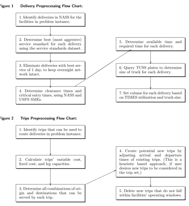
• Deliveries:The goal of the deliveries preprocessing step is to identify the parameters necessary for defining a delivery, and output a standardized data set for use in the optimization model (cf. Section 5.2). In order to obtain all the parameters, data is pulled from USPS systems (e.g., the National Air and Surface System (NASS), the Transportation Information Management Evaluation System (TIMES), and the Transportation Contract Support System (TCSS); see http://www.
usps.com/foia/majorsys/networkop1.htm for details) as well as manually collected from USPS
Subject Matter Experts (SME). Figure 1 gives a summarized flow chart of the process done to complete the deliveries preprocessing.
• Trips: The goal of the trips preprocessing step is to identify the parameters necessary for defining a trip (cf. Section 5.2), and output a standardized data set for use in the optimization model. The trips can be either existing or newly created trips. In order to satisfy all the parameters, data is pulled from USPS systems (NASS, TIMES, and TCSS), as well as manually collected from USPS SMEs. Figure 2 gives a summarized flow chart of the process done to complete the trips preprocessing.
• Deliveries - Trips Crosswalk: Prior to running the optimization model, it is necessary to con-duct a preprocessing step to identify which trips are feasible for which deliveries. This is completed for each individual delivery, to identify the specific trips that are viable options from which the optimization can choose to transport that delivery. A trip is deemed feasible if it departs the origin facility at or after the delivery’s available time and arrives at the required destination facility at or before the delivery’s required time.
Figure 1 Delivery Preprocessing Flow Chart: 1. Identify deliveries in NASS for the facilities in problem instance.
²
²
2. Determine best (most aggresive) service standard for each delivery using the service standards dataset.
²
²
5. Determine available time and required time for each delivery.
²
²
3. Eliminate deliveries with best ser-vice of 1 day, to keep overnight net-work intact.
²
²
6. Query TCSS plates to determine size of truck for each delivery.
²
²
4. Determine clearance times and critical entry times, using NASS and USPS SMEs.
8
8
7. Set volume for each delivery based on TIMES utilization and truck size.
Figure 2 Trips Preprocessing Flow Chart: 1. Identify trips that can be used to route deliveries in problem instance.
²
²
2. Calculate trips’ variable cost, fixed cost, and leg capacities.
²
²
4. Create potential new trips by adjusting arrival and departure times of existing trips. (This is a heuristic based approach, if user desires new trips to be considered in the trip set.)
²
²
3. Determine all combinations of ori-gin and destinations that can be served by each trip.
6
6
5. Delete new trips that do not fall within facilities’ operating windows.
5.2. Optimization Model Inputs
As previously discussed, the three underlying components of the HCAP model structure are facil-ities, deliveries (i.e., mail volumes between pairs of facilities), and trips among the facilities. The optimization model (cf. Section 4) requires the following specific inputs to define an instance of the HCAP model.
• List of facilities:The facility list identifies all facilities that will be included in the analysis. The HCAP model can handle many different types of facilities, such as PDCs, BMCs, PMPCs, AMCs, STCs, major mailers, and others. The set of facilities included within a single analysis, however, should be selectively chosen such that it represents a logical component of a transportation network. In other words, the pickup and delivery relationships between all facilities in the facility list should make sense, and the inter-relationships among facilities should be well-defined. Depending on the nature of the transportation network, each facility may serve as an origin facility, a destination
facility, or both. The characteristics that differentiate between origin and destination facilities are specified in the data inputs for deliveries between facility pairs.
• List of deliveries between facility pairs: The HCAP model optimizes the selection of trips among facilities to minimize the total transportation costs while meeting all delivery requirements. Each delivery is defined as a specific volume of mail that requires transport from an origin facility to a destination facility. The following characteristics of the deliveries are used in the HCAP model:
— The origin facility (the location at which the mail is to be picked up). — The time at which the mail is available at the origin facility.
— The destination facility (the location to which the delivery must be delivered). — The time at which the delivery is required at the destination facility.
— The volume of the delivery.
— Whether or not the delivery is splitable (cf. the deliveries item in Section 4).
Notice that, in practice, different mail classes may have different available times or different delivery time requirements. In that case, separate deliveries may be defined for each mail class. For example, for the mail going from a single origin facility to a single destination facility one may define different deliveries for First Class mail, Priority mail, Standard mail, and Packaged Services mail. However, it may be possible (and preferable) to combine multiple mail classes into a single delivery in cases where they share the same availability time and the same required delivery time for a specific origin-destination pair.
• Feasible trips among facilities: Each delivery specifies a volume of mail that must be trans-ported from a specific origin facility to a specific destination facility, within a certain time window. For each delivery, there are certain existing trips and a potential number of new (but defined) trips that could transport the mail from the origin facility to the destination facility. These trips may travel directly from the origin to the destination (i.e., a one leg trip), or they could stop at one or more other facilities along the way (i.e., a trip with various legs). For each delivery, a set of
feasible trips must be specified; that is, the set of all possible trips in which the delivery can be transported from the origin to the destination within the delivery’s time window. For each of these feasible trips, the following characteristics must be provided:
— The origin facility. — The destination facility.
— All stops (i.e., legs) along the trip between origin and destination. — The transportation capacity on each leg along the trip.
— The fixed transportation cost of the trip.
— The variable transportation cost (i.e., cost per unit of volume) on each leg along the trip. Trips generally will have the same capacity on all legs along the trip, as the truck size will remain unchanged. However, as previously discussed (see Capacity Constraints item in Section 4), different leg capacities might be used to take into account mail deliveries (not in the model) that have been already assigned to some of the trip legs. Variable cost may also be the same on all legs along the trip, or variable cost may often be zero if the cost structure is such that the trip incurs a single fixed cost (possibly based on mileage of the trip) for utilizing the trip.
5.3. Solution of HCAP VRP/PD model
A C++ program was developed that reads the information in the optimization model inputs to construct the HCAP VRP/PD MIP (cf. Section 4) such that it can be solved by the CPLEX optimization library. This code also generates the relevant optimization model outputs from the CPLEX solution information.
5.4. Optimization Model Outputs and Postprocessing
The optimization model identifies the optimal set of trips that can satisfy all delivery requirements. The output from the optimization model is therefore the subset of trips that should be utilized in an optimized scenario, and the optimal assignment of each delivery to the appropriate trip(s). The optimization model also returns the total transportation cost for the optimal assignment. The HCAP model post-processes this raw output information to produce several final reports for the analysis of USPS decision makers. In addition to the optimization model inputs and outputs, mapping files are used to associate the deliveries and trips with NASS specific information and to link the deliveries to their assigned trips.
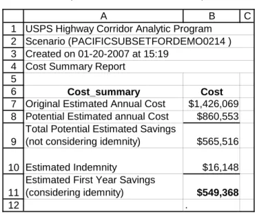
• Cost Summary Report: The Cost Summary Report summarizes the potential cost savings that USPS could realize by implementing the optimized trip recommendations identified by the HCAP model. These cost savings represent the potential annual decrease in transportation costs for the set of transportation modeled, resulting from trip consolidation opportunities. A sample Cost Summary Report is provided in Figure 3.
Figure 3 Sample Cost Summary Report (formatted for display purposes):
1 2 3 4 5 6 7 8 9 10 11 12 A B C Cost_summary Cost
Original Estimated Annual Cost $1,426,069 Potential Estimated annual Cost $860,553 Total Potential Estimated Savings
(not considering idemnity) $565,516 Estimated Indemnity $16,148 Estimated First Year Savings
(considering idemnity) $549,368
. USPS Highway Corridor Analytic Program Scenario (PACIFICSUBSETFORDEMO0214 ) Created on 01-20-2007 at 15:19
Cost Summary Report
In particular, this report presents the annual transportation costs associated with the baseline scenario, the annual costs associated with the optimized set of transportation, and the corre-sponding annual savings that could be attained by implementing the model recommendations. The indemnity cost is the penalty that USPS would have to pay for early termination of established contracts; this penalty is considered within the HCAP optimization when identifying the optimal solution. The Estimated First Year Savings represents the expected annual savings considering any penalty costs for indemnity.
• Operational Summary Report:The Operational Summary Report presents information about the number of trips included in the scenario. This report shows the number of trips in the scenario, the number of trips recommended for elimination (by consolidating their mail volumes onto other trips) and the number of remaining trips that have mail added to them (from the eliminated trips). Sample information from this report is provided in Figure 4.
Similar to the Cost Summary Report, these numbers are calculated by comparing the trips in the baseline set with the trips in the optimization results, to determine the number of trips that could be eliminated through consolidation opportunities.
Figure 4 Sample Operational Summary Report (formatted for display purposes): 1 2 3 4 5 6 9 13 14 16 17 B C D Operational_Summary Trips Total Number of Trips in Scenario 46 Number of Trips Recommended for Elimination 16 Number of Trips with Volume Added 14 Number of Trips Not Adjusted in Model Run 16 USPS Highway Corridor Analytic Program
Scenario (PACIFICSUBSETFORDEMO0214 ) Created on 01-20-2007 at 15:21
Operational Summary Report
• Utilization Summary Report:The Utilization Summary Report displays the change in average trip utilization that would result by implementing the optimization results. Increased utilization is typically desirable, since low utilization often indicates excess capacity that is paid for but is not being used to transport mail volumes. By consolidating mail onto fewer trips through optimization the average utilization on the trucks being used typically increases, and this report presents that information. A sample Utilization Summary Report is provided in Figure 5.
Figure 5 Sample Utilization Summary Report (formatted for display purposes):
1 2 3 4 5 6 7 8 10 11 12 13 A D E Utilization_Summary
Original Average Utilization 63% New Potential Average Utilization 85% Number of Trips with an Increase in Utilization 13 Number of Trips with a Decrease in Utilization 0 Number of Trips with No Change in Utilization 17
. USPS Highway Corridor Analytic Program
Scenario (PACIFICSUBSETFORDEMO0214 ) Created on 01-20-2007 at 15:20
Utilization Summary Report
The calculation for Original Average Utilization in this report is based on dividing the mail volumes on current (baseline) trucks into the capacities of those trucks, and the New Potential Average Utilization is calculated for the optimized set of trucks, similarly, by dividing the assigned volumes by capacities for that optimal set of trucks.
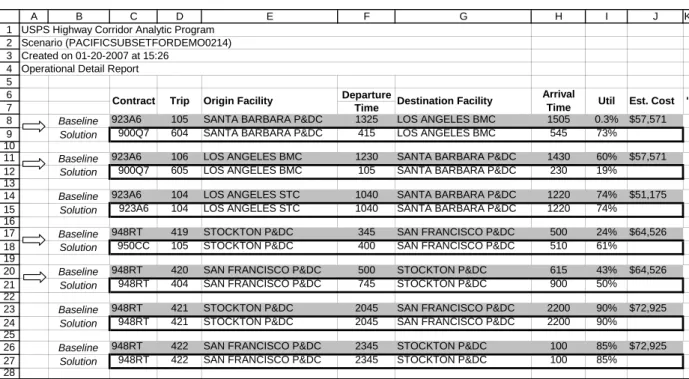
• Operational Detail Report: While the summary reports present information about overall statistics such as potential annual costs savings, trip elimination counts, and average utilization improvement percentages, the Operational Detail Report details how the transportation special-ists would actually implement the results recommended by the optimization output. This report displays each existing truck (from the baseline) side-by-side with the optimal assignment (i.e., how
specifically the mail that is currently being transported on that truck should be transported within the optimized condition). In many cases, the current truck remains within the optimized set and the optimal recommendation is merely to continue transporting that truck’s volume on that truck. In other cases, the truck can be eliminated and its mail can be consolidated onto another truck that has excess capacity, in which case the new truck assignment is indicated in the right side of the report, replacing the existing truck that is presented in the left side. Sample information from a subset of the Operational Detail Report is provided in Figure 61. (For purposes of displaying the
report information here, the report is reformatted such that the current trip is displayed in gray and the recommended trip is displayed in white below the current trip, rather than to the right of the current trip. The consolidation opportunities are highlighted with arrows in this figure.)
Figure 6 Sample Operational Detail Report (formatted for display purposes)
1 2 3 4 5 6 7 8 9 10 11 12 13 14 15 16 17 18 19 20 21 22 23 24 25 26 27 28 A B C D E F G H I J K Departure Time
Baseline 923A6 105 SANTA BARBARA P&DC 1325 LOS ANGELES BMC 1505 0.3% $57,571
Solution 900Q7 604 SANTA BARBARA P&DC 415 LOS ANGELES BMC 545 73%
Baseline 923A6 106 LOS ANGELES BMC 1230 SANTA BARBARA P&DC 1430 60% $57,571
Solution 900Q7 605 LOS ANGELES BMC 105 SANTA BARBARA P&DC 230 19%
Baseline 923A6 104 LOS ANGELES STC 1040 SANTA BARBARA P&DC 1220 74% $51,175
Solution 923A6 104 LOS ANGELES STC 1040 SANTA BARBARA P&DC 1220 74%
Baseline 948RT 419 STOCKTON P&DC 345 SAN FRANCISCO P&DC 500 24% $64,526
Solution 950CC 105 STOCKTON P&DC 400 SAN FRANCISCO P&DC 510 61%
Baseline 948RT 420 SAN FRANCISCO P&DC 500 STOCKTON P&DC 615 43% $64,526
Solution 948RT 404 SAN FRANCISCO P&DC 745 STOCKTON P&DC 900 50%
Baseline 948RT 421 STOCKTON P&DC 2045 SAN FRANCISCO P&DC 2200 90% $72,925
Solution 948RT 421 STOCKTON P&DC 2045 SAN FRANCISCO P&DC 2200 90%
Baseline 948RT 422 SAN FRANCISCO P&DC 2345 STOCKTON P&DC 100 85% $72,925
Solution 948RT 422 SAN FRANCISCO P&DC 2345 STOCKTON P&DC 100 85% USPS Highway Corridor Analytic Program
Scenario (PACIFICSUBSETFORDEMO0214) Created on 01-20-2007 at 15:26
Operational Detail Report
Arrival
Time Util Est. Cost ' Contract Trip Origin Facility Destination Facility
In the particular report shown in Figure 6, the optimization identified the opportunity to con-solidate Trip #105 of Contract 923A6 onto Trip #604 of Contract 900Q7. Elimination of that trip would save the annual cost of $57,571 (minus any applicable indemnity penalty).
6.
Results
HCAP has been fully developed and tested, and has been deployed to transportation analysts at USPS Headquarters and in the USPS Area offices. These transportation analysts are currently using HCAP to optimize transportation subsets throughout the U.S. to identify cost savings oppor-tunities. Each analyst is provided the flexibility within the HCAP model to define specific scenarios of interest, set the business constraints and model parameters, and analyze the results to develop recommendations for implementation. Several sample HCAP scenarios have already been com-pleted at USPS Headquarters and in the Area offices, and many of the recommendations from those scenarios have been implemented or are in the process of being implemented.
USPS Headquarters, the Pacific Area office, and IBM worked together during HCAP develop-ment to model the Pacific Area transportation network including transportation among P&DCs, BMCs, AMCs, and STCs. Many of the recommendations from this model run have already been implemented, resulting in approximately $3.7 million annual savings to-date. These savings rep-resent 24% of the cost of transportation that was eligible for elimination within the optimization model run. (In each model run, a portion of the trips are eligible for elimination and the rest are not. Eligibility depends on trip data availability and user-specified parameters.)
A separate scenario was developed for inbound and outbound transportation at an STC in the Midwest. The implementation of recommendations from that model run has resulted in approxi-mately $1.3 million annual savings to-date. The HCAP model was also recently used in the Eastern Area, as HCAP was adapted to model local transportation at a North Carolina P&DC and was used to model STC transportation in Pennsylvania. HCAP was responsible for helping identify approximately $400,000 annual savings in those efforts. Several other scenarios are currently in development at various other Area offices as well as at USPS Headquarters. In these scenarios, transportation analysts are exploring many different applications of the HCAP model, including using HCAP for renewal period to identify which trips should be renewed and which trips may be consolidated with other trips, planning for the holiday peak season, and helping identify alternative solutions in STC transportation planning.
7.
Conclusion
USPS operates an extremely large and complex transportation network and, accordingly, trans-portation planning is a critical yet challenging facet of USPS Logistics. USPS is proactively devel-oping a comprehensive set of analytic capabilities using advanced modeling techniques, to assist in the transportation planning process. HCAP is an optimization model that USPS and IBM designed and developed to identify savings opportunities in USPS highway transportation. The HCAP model has been fully developed, tested, and deployed to transportation analysts at USPS Headquarters and in the regional Area offices. HCAP has been used to model many different subsets of USPS highway transportation, and many of the model results have been implemented, resulting in annual savings already being realized by USPS.
Appendix. Mathematical Formulation of the USPS HCAP problem
The HCAP mathematical programming formulation uses the following basic model variables and param-eters:
Index Sets
I set of all deliveries,
R set of all trips,
Kr set of all legs on tripr∈ R,
U set of all unsplitable deliveries (i.e., deliveries that have to be routed on a single trip). Parameters
Vi volume of deliveryi∈ I, Fr fixed cost for using tripr∈ R,
Crk cost per unit of volume routed on legk∈ Kr of tripr∈ R, Srk capacity (in units of volume) of legk∈ Kr of trip r∈ R, Air
½
1 if deliveryi∈ I can be routed on tripr∈ R, 0 otherwise,
Birk ½
1 ifAir= 1 and deliveryi∈ I uses legk∈ Kr of tripr∈ Rwhen routed on tripr, 0 otherwise.
yr ½
1 if tripr∈ Ris used, 0 otherwise,
xir proportion of delivery’si∈ I volume that is routed using trip r∈ R. Basic MIP formulation
Minimize X r∈R Ã Fryr+X k∈Kr X i∈I BirkCrkVixir ! subject to X r∈R Airxir= 1 ∀i∈ I, (C.1) X i∈I
BirkVixir≤Srkyr ∀r∈ R,∀k∈ Kr,(C.2)
xir≤yr ∀r∈ R,∀i∈ I, (C.3)
0≤xir≤1 ∀r∈ R,∀i6∈ U, (C.4)
yr∈ {0,1}, xir∈ {0,1} ∀r∈ R,∀i∈ U. (C.5)
(1)
The objective of this MIP formulation is to minimize the total cost of routing the deliveries on the available trips. This cost includes the fixed cost incurred for the use of any trip, and the variable cost incurred for routing the volume of the deliveries on particular legs of the trips. Constraint (C.1) ensures that 100% of every delivery’s volume is routed on one or (if the delivery is not unsplitable) more of the trips in which the delivery can be routed. Constraint (C.2) ensures that the total volume routed on all legs of the used trips (i.e., whenyr= 1) is less than or equal to the capacity of the legs. The right hand side of (C.2) makes the capacity of legs in unused trips (i.e., whenyr= 0) equal to zero. The multiplication of the leg capacities by the trip variables in the right hand side of (C.2) is simply done to strengthen the MIP formulation of the problem. Constraint (C.3) ensures that deliveries (or percentages of deliveries) are routed only on used trips. Strenghtening constraints
In order to further strengthen this MIP formulation, two major types of constraints are incorporated to the formulation:
1. Symmetry breaking constraints: To construct the MIP formulation (1), it is necessary to generate the trips in advance (as opposed to other vehicle routing applications that generate trips as needed, like that of M. Desrochers (1992)). Given that it is unclear exactly what trips are needed in the formulation, it is likely that multiple, similar trips will be added to the formulation. These trips can hopelessly slow down a MIP solver by burdening it to explore and eliminate many alternative equivalent solutions, so-called symmetric solutions (cf. Sherali and Smith (2001)). To avoid this problem, we rank trips as follows: Consider two specific trips; for example, tripAand tripB. If
(a) the fixed cost of tripAis less than or equal to the fixed cost of tripB, and
(b) the variable cost (per unit of volume routed) of each leg of tripAis less than or equal to the variable cost of tripB, and
(c) the set of deliveries that can be routed on tripBis a subset of those that can be routed on tripA, then it is considered that trip A dominatestrip B. If tripA dominates trip B, and tripB dominates trip A, then tripsAandBareequivalent. If tripAdominates tripB, we can add the constraint
yA≥yB
to the basic MIP formulation of the problem (1) without deleting any optimal solutions. In doing so, we remove the symmetry between tripAand tripB, making the solution process much more efficient. If tripsA
andBare equivalent, we can break the tie arbitrarily, as long as it is done consistently. In practice we break ties in order of appearance in the input data file.
2. Knapsack constraints:Consider any set of deliveries D ⊆ I. LetR(D) be the set of trips in which at least one of the deliveries in D can be routed. For each trip r in R(D), let S∗
of any leg of tripr that can be used by a delivery inD. Then, the knapsack constraint(cf. Nemhauser and Wolsey (1988)) X r∈R(D) S∗ ryr≥ X i∈D Vi
is a valid constraint for this problem. As given, this constraint does not strengthen the formulation. However, modern integer programming optimizers recognize the form of this constraint and are able to add cover inequalities (cf. Nemhauser and Wolsey (1988)) and other constraints to strengthen the integer program. These redundant constraints generally create models that are easier to solve (see, e.g., Aardal (1998)). There are a number of choices to construct sets D; for example D can be the set of all deliveries that have the same origin and destination. In practice, we add a knapsack constraint to the basic MIP formulation of the problem (1) for every setDcorresponding to a pair of origin–destination in the problem.
The computational testing we did confirms the findings of Aardal (1998): it is the addition of these seemingly redundant constraints that is key to the effective solution to this model.
References
Aardal, K. 1998. Reformulation of capacitated facility location problems: How redundant information can help. Annals of Operations Research 82(1) 289–309.
Bodin, L., B. Golden. 1981. Classification in vehicle routing and scheduling. Networks 11(2) 97–108. Drezner, Z. 1995. Facility Location: A Survey of Applications and Methods. Springer.
M. Desrochers, M. Solomon, J. Desrosiers. 1992. A new optimization algorithm for the vehicle routing problem with time windows. Operations Research 40(2) 342–354.
Nemhauser, G. L., L. A. Wolsey. 1988. Integer and combinatorial optimization. John Wiley and Sons. Sherali, H. D., J. Cole Smith. 2001. Improving discrete model representations via symmetry considerations.