The Wealth-Consumption Ratio
∗
Hanno Lustig
UCLA Anderson and NBER
Stijn Van Nieuwerburgh
NYU Stern, NBER, and CEPR
Adrien Verdelhan
MIT Sloan and NBER
∗Lustig: Department of Finance, UCLA Anderson School of Management, Box 951477, Los Angeles,
CA 90095; [email protected]; Tel: (310) 206-6077;http://www.anderson.ucla.edu/x18962.xml. Van Nieuwerburgh: Department of Finance, Stern School of Business, New York University, 44 W. 4th Street, New York, NY 10012; [email protected]; Tel: (212) 998-0673; http://www.stern.nyu.edu/~svnieuwe. Verdelhan: MIT Sloan, [email protected]; http://web.mit.edu/adrienv/www/. The authors would like to thank Dave Backus, Geert Bekaert, John Campbell, John Cochrane, Ricardo Colacito, Pierre Collin-Dufresne, Bob Dittmar, Greg Duffee, Darrell Duffie, Robert Goldstein, Lars Peter Hansen, John Heaton, Dana Kiku, Ralph Koijen, Martin Lettau, Francis Longstaff, Sydney Ludvigson, Thomas Sargent, Kenneth Singleton, Stanley Zin, and participants of the NYU macro lunch, seminars at Stanford GSB, NYU finance, BU, the University of Tokyo, LSE, the Bank of England, FGV, MIT Sloan, Purdue, LBS, Baruch, Kellogg, Chicago GSB, Wharton, and conference participants at the SED in Prague, the CEPR meeting in Gerzensee, the EFA meeting in Ljubljana, the AFA and AEA meetings in New Orleans, the NBER Asset Pricing meeting in Cambridge, and the NYU Five Star Conference for comments. This work was supported by the National Science Foundation [grant number 0550910].
Abstract
We derive new estimates of total wealth, the returns on total wealth, and the wealth effect on consumption. We estimate the prices of aggregate risk from bond yields and stock returns using a no-arbitrage model. Using these risk prices, we compute total wealth as the price of a claim to aggregate consumption. We find that U.S. households have a surprising amount of total wealth, most of it human wealth. This wealth is much less risky than stock market wealth. Events in long-term bond markets, not stock markets, drive most total wealth fluctuations. The wealth effect on consumption is small and varies over time with real interest rates.
The total wealth portfolio plays a central role in modern asset pricing theory and macroe-conomics. Total wealth includes real estate, non-corporate businesses, other financial assets, durable consumption goods, and human wealth. The objective of this paper is to measure the amount of total wealth, the amount of human wealth, and the returns on each. The conventional approach to approximating the return on total wealth is to use the return on an equity index. Our approach is to measure total wealth as the present discounted value of a claim to aggregate consumption. The discount factor we use is consistent with observed stock and bond prices. Our preference-free estimation imposes only the household budget constraint and no-arbitrage conditions on traded assets. According to our estimates, stock market wealth is only 1% of total wealth while all non-human wealth only 8%. Moreover, the returns on the vast majority of total wealth differ markedly from equity returns; they are much lower on average and have low correlation with equity returns. Thus, our results challenge the conventional approach.
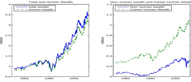
Our main finding is that households in the United States have a surprising amount of total wealth, $3.5 million per person in 2011 (in 2005 dollars). Of this, 92% is human wealth, the discounted value of all future U.S. labor income. Our estimation imputes a value of $1 million to an average career spanning 35 years. The high value of total wealth is reflected in a high average wealth-consumption ratio of 83, much higher than the average equity price-dividend ratio of 26. Equivalently, the total wealth portfolio earns a much lower risk premium of 2.38% per year, compared to an equity risk premium of 6.41%. Total wealth returns are only half as volatile as equity returns. The lower variability in the wealth-consumption ratio indicates less predictability in total wealth returns. Unlike stocks, most of the variation in future expected total wealth returns is variation in future expected risk-free rates, and not variation in future expected excess returns. The correlation between total wealth returns and stock returns is only 27%, while the correlation with 5-year government bond returns is 94%. Thus, the destruction and creation of wealth in the U.S. economy are largely disconnected from events in the stock market and are related to events in the bond markets instead.
Between 1979 and 1981 when real interest rates rose, $318,000 of per capita wealth was destroyed. Afterwards, as real yields fell, real per capita wealth increased steadily from $860,000 in 1981 to $3.5 million in 2011. Total U.S. household wealth was hardly affected by the spectacular declines in the stock market in 1973-1974, 2000-2001, and 2007-2009. The main message from these results is that equity is quite different from the total wealth portfolio.
A simple back-of-the-envelope Gordon growth model calculation helps explain the high wealth-consumption ratio. The discount rate on the consumption claim is 3.51% per year (a consumption risk premium of 2.38% plus a risk-free rate of 1.49% minus a Jensen term of 0.37%) and its cash-flow growth rate is 2.31%. The Gordon growth formula delivers the estimated mean wealth-consumption ratio: 83 = 1/(.0351−.0231).
In addition to the low volatility of aggregate consumption growth innovations, the reason that total wealth resembles a real bond is that the value of a claim to aggregate risky consumption is similar to that of a claim whose cash flows grow deterministically at the average consumption growth rate. The latter occurs because innovations to current and future consumption growth carry a small market price of risk according to our calculations. This is not a foregone conclusion because the market prices of risk are estimated to be consistent with observed stock and bond prices. The finding that current consumption growth innovations are assigned a small price is not a complete surprise. That is the equity premium puzzle. But, we also know that traded asset prices predict future consumption growth. This opens up the possibility that shocks to future consumption demand a high risk compensation. A key finding of our work is that this channel is not strong enough to generate a consumption risk premium that resembles anything like the equity risk premium. Discounting consumption at a low rate of return implies that the present discounted value of the stream (total wealth) is high, arguably higher than commonly believed.
Our methodology also produces new estimates of the marginal propensity to consume out of wealth. We find that the U.S. consumer spent only 0.76 cents out of the last dollar
of wealth, on average over our sample period. The marginal propensity to consume tracks interest rates: It peaks in 1981 at 1.4 cents per dollar and bottoms out in 2010 at 0.6 cents per dollar. The 50% drop in the marginal propensity to consume out of wealth occurred because the newly created wealth between 1981 and 2010 reflected almost exclusively lower discount rates rather than higher future consumption growth. We estimate that all variation in the wealth-consumption ratio is due to variation in discount rates.
A key assumption in the paper is that stock and bond returns span all priced sources of risk. We verify that our unspanned consumption growth innovations are essentially acyclical and serially uncorrelated. In addition, we check whether the pricing of consumption inno-vations that are not spanned by innoinno-vations to bond yields or stock returns can overturn our results. Even if we allow for unspanned priced risk that delivers Sharpe ratios equal to four times the observed Sharpe ratio on stocks, the consumption risk premium remains 2.5 percentage points below the equity risk premium. In the Online Appendix, we show that our valuation procedure is appropriate even in an economy with heterogeneous agents who face uninsurable labor income risk, borrowing constraints, and limited asset market participation. To derive our wealth estimates, we use a vector auto-regression (VAR) model for the state variables as in Campbell (1991, 1993, 1996). We combine the estimated state dynamics with a no-arbitrage model for the stochastic discount factor (SDF). As in Duffie and Kan (1996), Dai and Singleton (2000), and Ang and Piazzesi (2003), the log SDF is affine in innovations to the state vector while market prices of aggregate risk are affine in the same state vector. We estimate the market prices of risk by matching salient features of nominal bond yields, equity returns and price-dividend ratios, and expected returns on factor-mimicking portfolios, linear combinations of stock portfolios that have the highest correlations with consumption and labor income growth. This approach is similar to that in Bekaert, Engstrom, and Xing (2009), Bekaert, Engstrom, and Grenadier (2010), and Lettau and Wachter (2011), who use affine models to match features of stocks and bonds. By using precisely-measured stock and bond price data, our approach avoids using data on housing, durable, and private business
wealth from the Flow of Funds. These wealth variables are often measured at book values and with substantial error.
Our approach also avoids making arbitrary assumptions on the expected rate of return (discount rate) of human wealth, which is unobserved. In earlier work, Campbell (1993), Shiller (1995), Jagannathan and Wang (1996), and Lettau and Ludvigson (2001a, 2001b) all make particular, and very different, assumptions on the expected rate of return on human wealth. In a precursor paper, Lustig and Van Nieuwerburgh (2008) back out human wealth returns to match properties of consumption data. Bansal, Kiku, Shaliastovich, and Yaron (2012) emphasize the role of macro-economic volatility in a related exercise. Using market prices of risk inferred from traded assets, we obtain a new estimate of expected human wealth returns that fits none of the previously proposed models. We estimate human wealth to be 92% of total wealth. This estimate is consistent with Mayers (1972), who first pointed out that human capital forms a major part of the aggregate capital stock in advanced economies, and with Jorgenson and Fraumeni (1989), who also calculate a 90% human wealth share. Our result is also consistent with the share of human wealth obtained by Palacios (2011) in a calibrated version of his dynamic general equilibrium production model.
Our results differ from earlier attempts to measure the wealth-consumption ratio and the return to total wealth. Lettau and Ludvigson (2001a, 2001b) estimate cay, a measure of the inverse wealth-consumption ratio. Their wealth-consumption ratio has a correlation of 24% with our series. Alvarez and Jermann (2004) do not allow for time-varying risk premia and measure total wealth returns as a linear combination of equity portfolio returns. They estimate a smaller consumption risk premium of 0.2%, and hence a much higher average wealth-consumption ratio.
Our paper connects to the literature that studies the valuation of an asset for which one only observes the dividend growth and not the price. The retirement and social security literature studies related questions when it values claims to future labor income (e.g. De Jong 2008, Geanakoplos and Zeldes 2010, Novy-Marx and Rauh 2011).
Our paper also contributes to the large literature on measuring the propensity to consume out of wealth. The seminal work of Modigliani (1971) suggests that a one dollar increase in wealth leads to a five-percent increase in consumption. Similar estimates appear in text-books, models used by central banks, and in monetary and fiscal policy debates [see Poterba (2000) for a survey]. A wealth effect of five cents on the dollar implies a wealth-consumption ratio that is four times lower than our estimates, or equivalently, a consumption risk premium as high as the equity risk premium. Our first contribution to this literature is to propose a wealth effect on consumption that is much smaller than previously thought. Second, we are the first to provide an estimate consistent with the budget constraint and no-arbitrage restrictions.1 Third, we find that the dynamics of this wealth effect relate to the bond mar-ket rather than stock marmar-ket dynamics. This would explain the modest contraction in total wealth and aggregate consumption in response to the large stock market wealth destruction of 1973-1974 (e.g. Hall 2001). Our results are consistent with Bernanke and Gertler’s (2001) suggestion that inflation-targeting central banks should ignore movements in asset values that do not influence aggregate demand. We find that traded assets amount to a relatively small share of total wealth. As a result, their price fluctuations do not affect much consumer spending, the largest component of aggregate demand.
Finally, our work contributes to the consumption-based asset pricing literature. It offers a new set of moments to evaluate their empirical performance. Too often, such models are evaluated on their implications for equity returns. But the models’ primitives are the preferences and the dynamics of aggregate consumption growth. Moments of returns on the consumption claim are the most primitive asset pricing moments and should be the most informative for testing these models. In contrast, the dividend growth dynamics of stocks can be altered without affecting equilibrium allocations or prices of traded assets other than stocks; modeling them entails more degrees of freedom. This paper carries out a comparison
1
Ludvigson and Steindel (1999) and Lettau and Ludvigson (2004) start from the household budget con-straint but do not impose the absence of arbitrage, and assume a constant price-dividend ratio on human wealth.
of two leading endowment economy models: the external habit model of Campbell and Cochrane (1999) and the long-run risk model of Bansal and Yaron (2004). Our work also has implications for production-based asset pricing models. As Kaltenbrunner and Lochstoer (2010) point out, such models usually generate the prediction that the claim to dividends is less risky than the claim to consumption. Our results indicate that this is counterfactual and that stocks are special. Modeling realistic dividend dynamics (by introducing labor income frictions, operational leverage, or financial leverage) is necessary to reconcile the low consumption risk premium with the high equity risk premium.
The rest of the paper is organized as follows. Section 1 describes our measurement approach conceptually. Section 2 shows how we estimate the risk price parameters and Section 3 describes the results from that estimation. Section 4 investigates what features of the model are responsible for which results and investigates an annual instead of a quarterly version of our model. Section 5 studies the economic implications of our measurement exercise for the cost of consumption risk and the propensity to consume out of wealth. It also shows that our conclusions remain valid when there is priced unspanned consumption risk. Section 6 compares the properties of the wealth consumption ratio in the long-run risk and external habit models to the ones we estimate in the data. Finally, Section 7 concludes. An Online Appendix describes our data, presents proofs, details the robustness checks, and shows that our valuation approach remains valid in an incomplete markets model.
1
Measuring the Wealth-Consumption Ratio in the Data
Section 1.1 describes the framework for estimating the wealth-consumption ratio and the return on total wealth. Section 1.2 presents two methodologies to compute the wealth-consumption ratio.
1.1
Model
The model consists of a state evolution equation and a stochastic discount factor.
1.1.1 State evolution equation
We assume that the N ×1 vector of state variables follows a Gaussian first-order VAR:
zt= Ψzt−1+ Σ
1 2ε
t, (1)
withεt∼i.i.d.N(0, I) and Ψ is aN×N matrix. The vectorz is demeaned. The covariance
matrix of the innovations is Σ; the model is homoscedastic. We use a Cholesky decomposition of the covariance matrix, Σ = Σ12Σ
1
2′, which has non-zero elements only on and below the
diagonal. We discuss the elements of the state vector in detail below. Among other elements, the state zt contains real aggregate consumption growth, the nominal short-term interest
rate, and inflation. Denote consumption growth by ∆ct = µc +e′czt, where µc denotes the
unconditional mean consumption growth rate and the N ×1 vector ec is the column of a N×N identity matrix that corresponds to the position of ∆cin the state vector. Likewise, the nominal 1-quarter rate is y$
t(1) =y$0(1) +e′ynzt, where y$0(1) is the unconditional average and eyn the selector vector. Similarly,πt=π0+e′πzt is the (log) inflation rate between t−1
and t. All lowercase letters denote logs. The next section contains details on the estimation of the VAR and Appendix A describes the data sources and definitions in detail.
1.1.2 Stochastic discount factor
We specify a stochastic discount factor (SDF) familiar from the no-arbitrage term structure literature, following Ang and Piazzesi (2003). The nominal pricing kernelM$
t+1 = exp(m$t+1) is conditionally log-normal: m$t+1 = −y$t(1)− 1 2Λ ′ tΛt−Λ′tεt+1. (2)
The real pricing kernel is Mt+1 = exp(mt+1) = exp(m$t+1 +πt+1); it is also conditionally Gaussian.2 The innovations in the vector ε
t+1 are associated with a N ×1 market price of risk vector Λt of the affine form:
Λt = Λ0+ Λ1zt,
The N ×1 vector Λ0 collects the average prices of risk while the N ×N matrix Λ1 governs the time variation in risk premia.
1.2
The wealth-consumption ratio
We explore two methods to measure the wealth-consumption ratio. The first one uses con-sumption strips and avoids any approximation while the second approach builds on the Campbell (1991) approximation of log returns.
1.2.1 Consumption strips
A consumption strip of maturityτ pays realized consumption at periodτ, and nothing in the other periods. Under a no-bubble constraint on total wealth, the wealth-consumption ratio is the sum of the price-dividend ratios on consumption strips of all horizons (Wachter 2005):
Wt Ct =ewct = ∞ X τ=0 Ptc(τ), (3) where Pc
t(τ) denotes the price of a τ period consumption strip divided by the current
con-sumption. Appendix B proves that the log price-dividend ratio on consumption strips are affine in the state vector and shows how to compute them recursively.
If consumption growth were unpredictable and its innovations carried a zero risk price, then consumption strips would be priced like real zero-coupon bonds.3 The consumption
2Note that the consumption-CAPM is a special case of this, wherem
t+1= logβ−αµc−αηt+1andηt+1
denotes the innovation to real consumption growth andαthe coefficient of relative risk aversion.
3First, if aggregate consumption growth is unpredictable, i.e.,e′cΨ = 0, then innovations to future
con-sumption growth are not priced. Second, if prices of current concon-sumption risk are zero, i.e.,e′cΣ12Λ
1= 0 and
strips’ dividend-price ratios would equal yields on real bonds (with the coupon adjusted for growth µc). In this special case, all variation in the wealth-consumption ratio would be
traced back to the real yield curve.
1.2.2 Total wealth returns
Consumption strips allow for an exact definition of the wealth-consumption ratio, but they call for the estimation of an infinite sum of bond prices. A second approximate method delivers both a more practical and elegant definition of the wealth-consumption ratio. In our empirical work, we check that both methods deliver similar results.
In our exponential-Gaussian setting, the log wealth-consumption ratio is an affine func-tion of the state variables. To show this result, we start from the aggregate budget constraint:
Wt+1 =Rct+1(Wt−Ct). (4)
The beginning-of-period (or cum-dividend) total wealth Wt that is not spent on aggregate
consumption Ctearns a gross returnRct+1 and leads to beginning-of-next-period total wealth
Wt+1. The return on a claim to aggregate consumption, the total wealth return, can be written as: Rct+1 = Wt+1 Wt−Ct = Ct+1 Ct W Ct+1 W Ct−1 .
We use the Campbell (1991) approximation of the log total wealth return rc
t = log(Rct)
around the long-run average log wealth-consumption ratio Ac
0 ≡E[wt−ct],4
rtc+1 ≃κc0+ ∆ct+1+wct+1−κc1wct. (5)
The linearization constants κc
0 and κc1 are non-linear functions of the unconditional mean 4
wealth-consumption ratio Ac0: κc1 = e Ac 0 eAc 0 −1 >1 and κ c 0 =−log eA c 0 −1+ e Ac 0 eAc 0 −1A c 0. (6)
Proposition 1. The log wealth-consumption ratio is approximately a linear function of the (demeaned) state vector zt:
wct≃Ac0+Ac1′zt,
where the mean log wealth-consumption ratio Ac
0 is a scalar and Ac1 is the N ×1 vector, which jointly solve:
0 = κc0 + (1−κc1)Ac0+µc−y0(1) + 1 2(ec +A c 1)′Σ(ec+Ac1)−(ec+Ac1)′Σ 1 2 Λ0−Σ 1 2′e π (7) 0 = (ec +eπ +Ac1)′Ψ−κc1A1c′−e′yn −(ec +eπ +Ac1)′Σ 1 2Λ 1. (8)
The proof in appendix B conjectures an affine function for the log wealth-consumption ratio, imposes the Euler equation for the log total wealth return, and solves for the coefficients of the affine function as verification of the conjecture. The resulting expression for wctis an
approximation only because it relies on the log-linear approximation of returns in equation (5). This log-linearization is the only approximation in our procedure. Once we estimate the market prices of risk Λ0 and Λ1 below, equations (7) and (8) allow us to solve for the mean log wealth-consumption ratio (Ac
0) and its dependence on the state (Ac1).5
5Equations (7) and (8) form a system ofN+ 1 non-linear equations inN+ 1 unknowns. It is a non-linear
1.2.3 Consumption risk premium
Proposition 1 and the total wealth return definition in (5) jointly imply the following log total wealth return:
rtc+1 = r0c+ [(ec +Ac1)′Ψ−κc1Ac1′]zt+ (e′c +Ac1′)Σ
1 2ε
t+1, (9)
r0c = κc0+ (1−κc1)Ac0+µc, (10)
where equation (10) defines the unconditional mean total wealth returnrc
0. The consumption risk premium, the expected log return on total wealth in excess of the log real risk-free rate
yt(1) corrected for a Jensen term, follows from the Euler equation Et[Mt+1Rct+1] = 1:
Et rc,et+1 ≡Et rc t+1−yt(1) +1 2Vt[r c t+1] = −Covt rc t+1, mt+1 (11) = (ec+Ac1)′Σ 1 2 Λ0−Σ 1 2′e π + (ec +Ac1)′Σ 1 2Λ 1zt.
The first term on the last line is the average consumption risk premium. This is a key object of interest, which measures how risky total wealth is. The second (mean-zero) term governs the time variation in the consumption risk premium.
1.2.4 Growth conditions
Given the no-bubble constraint, there is an approximate link between the coefficients in the affine expression of the wealth-consumption ratio and the coefficients of the strip price-dividend ratios Pc t(τ) = exp(Ac(τ) +Bc(τ)′zt): exp(Ac0)≃ ∞ X τ=0
exp(Ac(τ)) and exp(Ac1)≃
∞
X τ=0
exp(Bc(τ)). (12)
A necessary condition for this first sum to converge and hence produce a finite average wealth-consumption ratio is that the consumption strip risk premia are positive and large
enough in the limit (as τ → ∞): (ec+Bc(∞))′Σ 1 2 Λ0−Σ 1 2e π > µc−y0(1) + 1 2(ec+B c( ∞))′Σ (ec+Bc(∞)).
We refer to this inequality as the growth condition. Because average real consumption growth
µc exceeds the average real short ratey0(1) in the data, the right-hand side of the inequality is positive. When all the risk prices in Λ0 are zero, this condition is obviously violated. It implies a lower bound for the consumption risk premium.
1.3
Human wealth
The same way we priced a claim to aggregate consumption, we price a claim to aggregate labor income. Human wealth is the present value of the latter claim. We impose that the conditional Euler equation for human wealth returns is satisfied and obtain a log price-dividend ratio, which is also approximately affine in the state: pdl
t = Al0 +Al1zt. (See
Proposition 2 in Online Appendix B.1.) By the same token, the conditional risk premium on the labor income claim is affine in the state vector (see equation B.5 in Online Appendix B.1).
2
Estimating the Market Prices of Risk
In order to recover the dynamics of the wealth-consumption ratio and of the return on wealth, we need to estimate the market prices of risk Λ0 and Λ1. This section details our estimation procedure. Section 2.1 describes the state vector. Section 2.2 lists the additional restrictions we impose on our framework. Section 2.3 describes the estimation technique.
To implement the model, we need to take a stance on what observables describe the aggregate dynamics of the economy. The de minimis state vector contains the nominal short rate, realized inflation, and the cash flow growth dynamics of the two cash flows this paper sets out to price: consumption and labor income. In this section, we lay out our
benchmark model, which contains substantially richer state dynamics than contained in these four variables. The richness stems from a desire to infer the market prices of risk from a model that accurately prices the bonds of various maturities, the equity market, and that takes into account some cross-sectional variation across stocks. Section 4 explores special cases of the benchmark model, with fewer state variables, in order to understand what elements are crucial for our main findings.
2.1
Benchmark state vector
Our benchmark state vector is:
zt= [CPt, yt$(1), πt, yt$(20)−y$t(1), pdmt , rtm, r f mpc
t , r
f mpy
t ,∆ct,∆lt]′.
The first four elements represent the bond market variables in the state, the next four represent the stock market variables, the last two variables represent the cash flows. The state contains in order of appearance: the Cochrane and Piazzesi (2005) factor (CP), the nominal short rate (yield on a 3-month Treasury bill), realized inflation, the spread between the yield on a 5-year Treasury note and a 3-month Treasury bill, the price-dividend ratio on the CRSP stock market, the real return on the CRSP stock market, the real return on a factor-mimicking portfolio for consumption growth, the real return on a factor-mimicking portfolio for labor income growth, real per capita consumption growth, and real per capita labor income growth. We recall that lower-case letters denote natural logarithms. This state vector is observed at quarterly frequency from 1952.I until 2011.IV (240 observations). In a robustness check, we also consider annual data from 1952 to 2011. The Cholesky decomposition of the residual covariance matrix, Σ = Σ12Σ
1
2′, allows us to interpret the shock
to each state variable as the sum of the shocks to all the preceding state variables and an own shock that is orthogonal to all previous shocks. Consumption and labor income growth are ordered after the bond and stock variables because we use the prices of risk associated
with the first eight innovations to value the consumption and labor income claims.
The goal of our exercise is to price claims to aggregate consumption and labor income using as much information as possible from traded assets. Thus, the choice of state variables is motivated by a desire to capture all important dynamics of bond and stock prices. Many of the state variables have a long tradition in finance as predictors of stock and bond returns.6
2.1.1 Expected consumption growth
Equally important is a rich specification of the cash flows we want to price: consump-tion and labor income growth. First, our state vector includes variables like interest rates (Harvey 1988), the price-dividend ratio, and the slope of the yield curve (Ang, Piazzesi, and Wei 2006) that have been shown to forecast future consumption growth. The predictability of future consumption growth by stock and bond prices whose own shocks carry non-zero prices of risk results in a risk premium to future consumption growth innovations and thus to create a wedge between the risky and the trend consumption claims. Having richly spec-ified expected consumption growth dynamics alleviates the concern that the model misses important (priced) shocks to expected consumption growth. Second, the modest correlation (29%) of the aggregate stock market portfolio with consumption growth motivates us to use additional information from the cross-section of stocks to learn more about contemporane-ous shocks to consumption and labor income claims. We use the 25 size- and value-portfolio returns to form a consumption growth factor-mimicking portfolio (FMP) and a labor income growth FMP. The consumption (labor income) growth FMP has a 36% (36%) correlation with actual consumption. Pricing these FMP well alleviates the concern that our model misses important shocks to current consumption innovations.
Our state variables zt explain 29% of variation in ∆ct+1. The volatility of annualized expected consumption growth is 0.49%, more than one-third of the volatility of realized 6For example, Ferson and Harvey (1991) study the yield spread, the short rate, and consumption growth
as predictors of stocks, while Cochrane and Piazzesi (2005) emphasize the importance of the CP factor to predict bond returns.
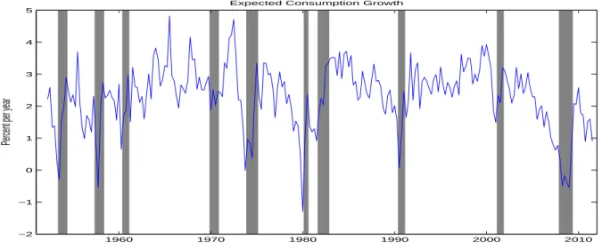
consumption growth, while the first-order autocorrelation of expected consumption growth is 0.70 in quarterly data. This shows non-trivial consumption growth predictability, in line with the literature. Figure 1 plots the (annualized) one-quarter-ahead expected consump-tion growth series implied by our VAR. The shaded areas are NBER recessions. Expected consumption growth experiences the largest declines during the Great Recession of 2007.IV-2009.II, the 1953.II-1954.II recession, the 1957.III-1958.II recession, the 1973.IV-1975.I reces-sion, the double-dip NBER recession from 1980.I to 1982.IV, and somewhat smaller declines during the less severe 1960.II-1961.I, 1990.III-1991.I, and 2001.I-2001.IV recessions. Hence, the innovations to expected consumption growth are highly cyclical. That cyclical risk, alongside the long-run risk in expected consumption growth implied by the VAR, should be priced in asset markets. Finally, most of the cyclical variation in consumption growth is captured by traded asset returns. The correlation of unspanned (orthogonal) consump-tion growth with the NBER dummy is only -0.01 and not statistically different from zero. Moreover, these unspanned innovations are essentially uncorrelated over time; the first-order autocorrelation is -0.05.
Figure 1: Consumption growth predictability
Percent per year
Expected Consumption Growth
1960 1970 1980 1990 2000 2010 −2 −1 0 1 2 3 4 5
The figure plots (annualized) expected consumption growth at quarterly frequency, as implied by the VAR model:Et[∆ct+1] =
µc+I′
2.2
Restrictions
With ten state variables and time-varying prices of risk, our model has many parameters. On the one hand, the richness offers the possibility to accurately describe bond and equity prices without having to resort to latent state variables. On the other hand, there is the risk of over-fitting the data. To guard against this risk and to obtain stable estimates, we impose restrictions on our benchmark estimation.
We start by imposing restrictions on the dynamics of the state variable, that is, in the companion matrix Ψ. Only the bond market variables – first block of four – govern the dynamics of the nominal term structure; Ψ11 below is a 4×4 matrix of non-zero elements. For example, this structure allows for the CP factor to predict future bond yields, or for the short-term yield and inflation to move together. It also imposes that stock returns, the price-dividend ratio on stocks, or the factor-mimicking portfolio returns do not predict future yields or bond returns; Ψ12 is a 4×4 matrix of zeroes. The second block of Ψ describes the dynamics of the log price-dividend ratio and log return on the aggregate stock market, which we assume depends on their own lags, as well as the lagged bond market variables. The elements Ψ21 and Ψ22 are 2×4 and 2×2 matrices of non-zero elements. This allows for aggregate stock return predictability by the short rate, the yield spread, inflation, the CP factor, the price-dividend ratio, and its own lag, all of which have been shown in the empirical asset pricing literature. The FMP returns in the third block have the same predictability structure as the aggregate stock return, so that Ψ31 and Ψ32 are 2×4 and 2×2 matrices of non-zero elements. In our benchmark model, consumption and labor income growth do not predict future bond and stock market variables; Ψ14, Ψ24, and Ψ34 are all matrices of zeroes. Finally, the VAR structure allows for rich cash flow dynamics: expected consumption growth depends on the first nine state variables and expected labor income growth depends on all lagged state variables; Ψ41, Ψ42, and Ψ43 are 2×4, 2×2, and 2×2 matrices of non-zero elements, and Ψ44 is a 2×2 matrix with one zero in the upper-right corner. In sum, our
benchmark Ψ matrix has the following block-diagonal structure: Ψ = Ψ11 0 0 0 Ψ21 Ψ22 0 0 Ψ31 Ψ32 0 0 Ψ41 Ψ42 Ψ43 Ψ44 .
Section 4 also explores various alternative restrictions on Ψ. These do not materially alter the dynamics of the estimated wealth-consumption ratio. We estimate Ψ by OLS, equation-by-equation, and we form each innovation as follows zt+1(·)−Ψ(·,:)zt. We compute their
(full rank) covariance matrix Σ.
The zero restrictions on Ψ imply zero restrictions on the corresponding elements of the market price of risk dynamics in Λ1. For example, the assumption that the stock return and the price-dividend ratio on the stock market do not predict the bond variables implies that the market prices of risk for the bond market shocks cannot fluctuate with the stock market return or the price-dividend ratio. The entries of Λ1 in the first four rows and the fifth and sixth column must be zero. Likewise, because the last four variables in the VAR do not affect expected stock and FMP returns, the prices of stock market risk cannot depend on the last four state variables. Finally, under our assumption that all sources of aggregate uncertainty are spanned by the innovations to the traded assets (the first eight shocks), the part of the shocks to consumption growth and labor income growth that is orthogonal to the bond and stock innovations is not priced. We relax this assumption in section 5.3. Thus, Λ1,41, Λ1,42, Λ1,43, and Λ1,44 are zero matrices. This leads to the following structure for Λ1:
Λ1 = Λ1,11 0 0 0 Λ1,21 Λ1,22 0 0 Λ1,31 Λ1,32 0 0 0 0 0 0 .
We impose corresponding zero restrictions on the mean risk premia in the vector Λ0: Λ0 = [Λ0,1, Λ0,2, Λ0,3 0]′, where Λ0,1 is 4×1, and Λ0,2 and Λ0,3 are 2×1 vectors.
The matrix Λ1,11contains the bond risk prices, Λ1,21and Λ1,22contain the aggregate stock risk prices, and Λ1,31and Λ1,32 contain the risk prices on the FMP of aggregate consumption and labor income growth. While all zeroes in Ψ lead to zeroes in Λ1 in the corresponding entries, the converse is not true. That is, not all entries of the matrices Λ1,11, Λ1,21, Λ1,22, Λ1,31, and Λ1,32 must be zero even though the corresponding elements of Ψ all are non-zero. Whenever we have a choice of which market price of risk parameters to estimate, we follow a simple rule: we associate zero risk prices with traded assets instead of non-traded variables. In particular, we set the rows corresponding to the prices of CP risk, inflation risk, and pdm risk equal to zero because these are not traded assets, while the rows
corresponding to the short rate, the yield spread, the stock market return, and the FMP returns are non-zero. Our final specification has five non-zero elements in Λ0 and 26 in Λ1 (two rows of four and three rows of six). This specification is rich enough for the model to match the time-series of the traded asset prices that are part of the state vector.
The structure we impose on Ψ and on the market prices of risk is not overly restric-tive. A Campbell-Shiller decomposition of the wealth-consumption ratio into an expected future consumption growth component (∆cH
t ) and an expected future total wealth returns
component (rH
t ), detailed in Appendix B, delivers the following expressions:
∆cHt =e′cΨ(κc1I −Ψ)−1zt and rHt = [(ec+Ac1)′Ψ−κc1A1c′] (κc1I−Ψ)−1zt.
Despite the restrictions on Ψ and Λt, both the cash flow component and the discount rate
component depend on all state variables. In the case of ∆cH
t , this is because expected
consumption growth depends on all lagged stock and bond variables in the state. In the case of rH
t , there is additional dependence through Ac1, which itself is a function of the first nine state variables. The cash flow component does not directly depend on the risk prices (other
than throughκc1), while the discount rate component depends on all risk prices of stocks and bonds through Ac
1. This flexibility implies that our model can theoretically accommodate a large consumption risk premium. This happens when the covariances between consumption growth and the other aggregate shocks are large and/or when the unconditional risk prices in Λ0 are sufficiently large. In fact, in our estimation, we choose Λ0 large enough to match the equity premium. A low estimate of the consumption risk premium and hence a high wealth-consumption ratio are not a foregone conclusion.
2.3
Estimation
We estimate Λ0 and Λ1 from the moments of bond yields and stock returns. We relegate a detailed discussion of the estimation strategy to Appendix B. While all moments pin down all market price of risk estimates jointly, it is useful to organize the discussion as if the estimation proceeded in four steps. These steps can be interpreted as delivering good initial guesses from which to start the final estimation.
The model delivers a nominal (and real) term structure where bond yields are affine functions of the state variables. In a first step, we estimate the risk prices in the bond market block Λ0,1 and Λ1,11 by matching the time series for the short rate, the slope of the yield curve, and the CP risk factor. Because of the block diagonal structure, we can estimate these risk prices separately. In a second step, we estimate the risk prices in thestock market block Λ0,2, Λ1,21, and Λ1,22 jointly with the bond risk prices, taking the estimates from the first step as starting values. Here, we impose that the model delivers expected excess stock returns similar to the VAR. In a third step, we estimate the FMP risk prices in the factor-mimicking portfolio block Λ0,3, Λ1,31, and Λ1,32taking as given the bond and stock risk prices. Again, we impose that the risk premia on the FMP coincide between the VAR and the SDF model. The stock and bond moments used in the first three steps exactly identify the 5 elements of Λ0 and the 26 elements of Λ1. In other words, given the structure of Ψ, they are all strictly necessary to match the levels and dynamics of bond yields and stock returns.
For theoretical as well as for reasons of fit, we impose several additional constraints. We obtain these constraints from matching additional nominal yields, imposing the present-value relationship for stocks, imposing a human wealth share between zero and one, and imposing the growth condition on the consumption claim. To avoid over-parametrization, we choose not to let these constraints identify additional market price of risk parameters. We re-estimate all 5 parameters in Λ0 and all 26 parameters in Λ1 in a final fourth step where we impose the constraints, starting from the third-step estimates. Our final estimates for the market prices of risk from the last-stage estimation are listed at the end of Appendix B alongside the VAR parameter estimates. The online Appendix B provides more detail on the over-identifying restrictions.
3
Estimation Results
We first verify that the model does an adequate job describing the quarterly dynamics of the bond yields and stock returns. We then study the variations in the total wealth and human wealth. In the interest of space, we present auxiliary figures in the Appendix.
3.1
Model fit for bonds and stocks
Our model fits the nominal term structure of interest rates reasonably well (Figure B.1). We match the 3-month yield exactly. For the 5-year yield, which is part of the state vector through the yield spread, the average pricing error is -1 basis point (bp) per year. The annualized standard deviation of the pricing error is only 33 bps, and the root mean squared error (RMSE) is 33 bps. For the other four maturities, the mean annual pricing errors range from -7 bps to +62 bps, the volatility of the pricing errors range from 33 bps to 58 bps, and the RMSE from 33 bps to 65 bps.7 While these pricing errors are somewhat higher than the ones produced by term-structure models, our model has no latent state variables and only 7Note that the largest errors occur on the 20-year yield, which is unavailable between 1986.IV and 1993.II.
two term structure factors (two priced sources of risk that we associate with the second and fourth shocks). It also captures the level and dynamics of long-term bond yields well, a part of the term structure rarely investigated, but important for our purposes of evaluation of a long-duration consumption claim. On the dynamics, the annual volatility of the nominal yield on the 5-year bond is 1.40% in the data and 1.35% in the model.
The model also does a good job of capturing the bond risk premium dynamics. The model produces a nice fit between the Cochrane-Piazzesi factor, a measure of the 1-year nominal bond risk premium, in model and data (see right panel of Figure B.2). The annual mean pricing error is -15 bps and standard deviation of the pricing error is 70 bps. The 5-year nominal bond risk premium, defined as the difference between the 5-5-year yield and the average expected future short-term yield averaged over the next five years, is also matched closely by the model (left panel of Figure B.2). The long-term and short-term bond risk premia have a correlation of 74%. Thus, our model is able to capture the substantial variation in bond risk premia in the data. This is important because the bond risk premium turns out to constitute a major part of the consumption risk premium and of the marginal cost of consumption fluctuations.
The model also manages to capture the dynamics of stock returns quite well. The model matches the equity risk premium that arises from the VAR structure (bottom panel of Figure B.3). The average equity risk premium (including Jensen term) is 6.41% per annum in the data, and 6.41% in the model. Its annual volatility is 3.31% in the data and 3.25% the model. The model, in which the price-dividend ratio reflects the present discounted value of future dividends, replicates the price-dividend ratio in the data quarter by quarter (top panel of Figure B.3).
As in Ang, Bekaert, and Wei (2008), the long-term nominal risk premium on a 5-year bond is the sum of a real rate risk premium (defined the same way for real bonds as for nominal bonds) and the inflation risk premium. The right panel of Figure B.4 decomposes this long-term bond risk premium (solid line) into a real rate risk premium (dashed line)
and an inflation risk premium (dotted line). The real rate risk premium becomes gradually more important at longer horizons. The left panel of Figure B.4 decomposes the 5-year yield into the real 5-year yield (which itself consists of the expected real short rate plus the real rate risk premium), expected inflation over the next 5-years, and the 5-year inflation risk premium. The inflationary period in the late 1970s-early 1980s was accompanied by high inflation expectations and an increase in the inflation risk premium, but also by a substantial increase in the 5-year real yield.8 Separately identifying real rate risk and inflation risk based on nominal term structure data alone is challenging.9 We do not have long enough data for real bond yields, but stocks are real assets that contain information about the term structure of real rates. They can help with the identification. For example, high long real yields in the late 1970s-early 1980s lower the price-dividend ratio on the stock market stock, which indeed was low in the late 1970s-early 1980s (top panel of Figure B.3). High nominal yields combined with high price-dividend ratios would have suggested low real yields instead.
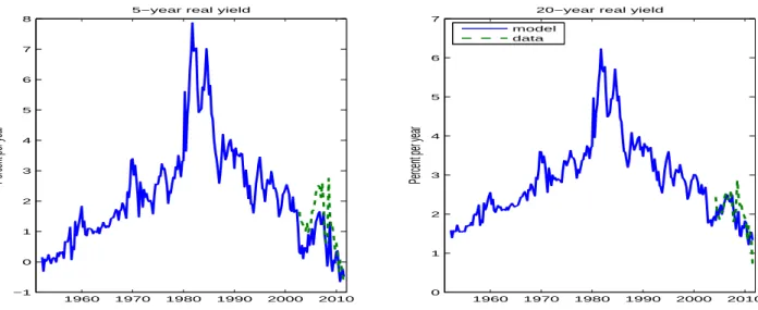
Average real yields range from 1.49% per year for 1-quarter real bonds to 2.87% per year for 20-year real bonds. Despite the short history of Treasury Inflation Indexed Bonds, potential liquidity issues early in the sample, and the dislocation in the TIPS market/rich pricing of nominal Treasuries (Longstaff, Fleckenstein, and Lustig 2010), it is nevertheless informative to compare model-implied real bond yields to observed real yields. Despite the fact that these real yields were not used in estimation, Figure 2 shows that the fit over the common sample is reasonably good both in terms of levels and dynamics.
Finally, the model matches the expected returns on the consumption and labor income growth FMP very well (Figure B.6). The annual risk premium on the consumption growth FMP is 1.08% in the data and model, with volatilities of 1.59% and 1.54%. Likewise, the 8Inflation expectations in our VAR model have a correlation of 76% with inflation expectations from the
Survey of Professional Forecasters (SPF) over the common sample 1981-2011. The 1-quarter ahead inflation forecast error series for the SPF and the VAR have a correlation of 79%. Realized inflation fell sharply in the first quarter of 1981. Neither the professional forecasters nor the VAR anticipated this decline, leading to a high realized real yield. The VAR expectations caught up more quickly than the SPF expectations, but by the end of 1981, both inflation expectations were identical.
9Many standard term structure models have a likelihood function with two local maxima with respect to
Figure 2: Dynamics of the real term structure of interest rates 1960 1970 1980 1990 2000 2010 −1 0 1 2 3 4 5 6 7 8
Percent per year
5−year real yield
1960 1970 1980 1990 2000 2010 0 1 2 3 4 5 6 7
Percent per year
20−year real yield model
data
The figure plots the observed and model-implied 5-, 7-, 10-, 20-, and 30-year real bond yields. Real yield data are constant maturity yields on Treasury Inflation Indexed Securities from the Federal Reserve Bank of St.-Louis (FRED II). We use the longest available sample for each maturity.
risk premium on the labor income growth FMP is 3.48% in data and model, with volatilities of 2.41% and 2.51%.
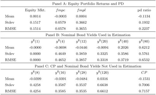
To summarize, Table 1 provides a detailed overview of the pricing errors on the assets used in estimation. Panel A shows the pricing errors on the equity portfolios; Panels B and C show the pricing errors on nominal bonds. Panel A shows that the volatility and RMSE of the pricing errors on the equity risk premium are about 15 bps per year; those on the factor-mimicking portfolio returns are 6 bps and 37 bps. Panel B shows the pricing errors on nominal bonds that were used in estimation. The 3-month rate is matched perfectly since it is in the state vector and carries no risk price. The pricing error on the 5-year bond is only 1 bp on average, with a standard deviation and RMSE of about 33 bps. One- through four-year yields have RMSEs between 39 bps and 46 bps per year. The 7-year bond has a RMSE of 35 bps, the 10-year bond one of 37 bps. The largest pricing errors occur on bonds of 20- and 30-year maturity, around 65 bps. One mitigating factor is that these bonds have some missing data over our sample period, which makes the comparison of yields in the model and data somewhat harder to interpret. Another is that there may be liquidity
effects at the long end of the yield curve that are not captured by our model. Finally, the RMSE on the CP factor is comparable to that on the 5-year yield once its annual frequency is taken into account.10
We conclude that our pricing errors are low given that we jointly price bonds and stocks, use no latent state variables, and include much longer maturity bonds than what is typically done in the literature.
Table 1: Pricing errors
This table reports the pricing errors on the asset pricing moments used in the estimation, as well as some over-identifying restrictions. The pricing error time series are computed as the difference between the predicted asset pricing moment by the model and the observed asset pricing moment in the data. The table reports time-series averages (Mean), standard deviations (Stdev), and root-mean squared errors (RMSE). Panel A reports pricing errors on the equity market portfolio, the consumption growth factor-mimicking portfolio (f mpc), and the labor income growth factor-mimicking portfolio (f mpl). It also reports how well the model matches the price-dividend ratio on the aggregate stock market. Panel B shows nominal bond yield pricing errors for the bond maturities that were used in estimation. Panel C shows bond yield errors for bond maturities that were not used in estimation, as well as the Cochrane-Piazzesi (CP) ratio. All moments are annualized and are multiplied by 100, except for the price-dividend ratio, which is annualized in levels.
Panel A: Equity Portfolio Returns and PD
Equity Mkt. f mpc f mpl pd ratio
Mean 0.0014 -0.0003 0.0004 -0.1134
Stdev 0.1517 0.0579 0.3662 0.1932
RMSE 0.1514 0.0578 0.3655 0.2237
Panel B: Nominal Bond Yields Used in Estimation
y$(1) y$(4) y$(12) y$(20) y$(40) y$(80)
Mean -0.0000 -0.0698 -0.0446 -0.0094 0.2026 0.6212 Stdev 0.0000 0.4649 0.3859 0.3325 0.3586 0.5761 RMSE 0.0000 0.4652 0.3857 0.3318 0.3719 0.6532
Panel C: CP and Nominal Bond Yields Not Used in Estimation
y$(8) y$(16) y$(28) y$(120) CP
Mean -0.0399 -0.0391 -0.0484 0.0316 -0.1531
Stdev 0.4258 0.3587 0.3537 0.6638 0.7006
RMSE 0.4254 0.3585 0.3535 0.6612 0.7157
3.2
The wealth-consumption ratio
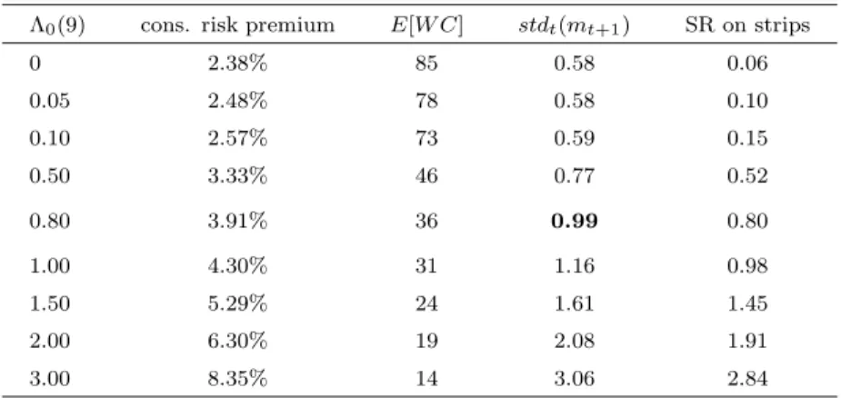
With the estimates for Λ0and Λ1 in hand, it is straightforward to use Proposition 1 and solve forAc
0 andAc1from equations (7)-(8). Table 2 summarizes the key moments of the log wealth-10The CP factor is constructed from annual returns while the yields are quarterly. To annualize the
volatility of yield pricing errors, we multiply the quarterly pricing errors by 2 =√4. To compare the two, the volatility and RMSE of CP should be divided by a factor of two.
consumption ratio obtained in quarterly data in column 3. The numbers in parentheses are small sample bootstrap standard errors, computed using the procedure described in Appendix B.9.
3.2.1 Comparison to stocks
We can directly compare the moments of the wealth-consumption ratio with those of the price-dividend ratio on equity. Thewc ratio has an annualized volatility of 19% in the data, considerably lower than the 29% volatility of the pdm ratio. The wc ratio in the data is
a persistent process; its 1-quarter (4-quarter) serial correlation is .97 (.87). This is similar to the .94 (.77) serial correlation of pdm. The annual volatility of changes in the wealth
consumption ratio is 4.51%, and because of the low volatility of aggregate consumption growth changes, this translates into a volatility of the total wealth return on the same order of magnitude (4.59%). The corresponding annual volatility of 9.2% is about half the 17.2% volatility of stock returns. The change in the wc ratio and the total wealth return have weak autocorrelation, suggesting that total wealth returns are hard to forecast by their own lags. The correlation between the (quarterly) total wealth return and consumption growth is mildly positive (.21).
How risky is total wealth compared to equity? According to our estimation, the con-sumption risk premium (calculated from equation 11) is 60 bps per quarter or 2.38% per year. This results in a mean wealth-consumption ratio of 5.81 in logs (Ac
0), or 83 in annual levels (exp{Ac
0−log(4)}). The consumption risk premium is only one-third as big as the eq-uity risk premium of 6.41%. Correspondingly, the wealth-consumption ratio is much higher than the price-dividend ratio on equity: 83 versus 26. A simple back-of-the-envelope Gordon growth model calculation sheds light on the mean of the wealth-consumption ratio. The discount rate on the consumption claim is 3.51% per year (a consumption risk premium of 2.38% plus a risk-free rate of 1.49% minus a Jensen term of 0.37%) and its cash-flow growth rate is 2.31%: 83 = 1/(.0351−.0231). The standard errors on the moments of the
wealth-consumption ratio and total wealth return are sufficiently small so that the corresponding moments of the price-dividend ratio or stock returns are outside the 95% confidence inter-val of the former. The main conclusion of our measurement exercise is that total wealth is (economically and statistically) significantly less risky than equity.
Table 2: Moments of the wealth-consumption ratio
This table displays unconditional moments of the log wealth-consumption ratiowc, its first difference ∆wc, and the log total wealth returnrc. The table also reports the time-series average of the conditional consumption risk premium, E[Et[rc,e
t ]],
whererc,edenotes the expected log return on total wealth in excess of the risk-free rate and corrected for a Jensen term. The
last row denotes the share of human wealth in total wealth. The first column reports moments from the long-run risk model (LRR model), simulated at quarterly frequency. All reported moments are averages and standard deviations (in parentheses) across the 5,000 simulations of 220 quarters of data. The second column reports the same moments for the external habit model (EH model). The last two columns report the data at quarterly and annual frequencies respectively. The standard errors are obtained by bootstrap, as described in Appendix B.9.
Moments LRR Model EH model data data
quarterly quarterly quarterly annual
Std[wc] 2.35% 29.33% 18.57% 24.68% (0.43) (12.75) (4.30) (7.81) AC(1)[wc] 0.91 0.93 0.97 (0.03) (0.03) (0.03) AC(4)[wc] 0.70 0.74 0.87 0.86 (0.10) (0.11) (0.08) (0.21) Std[∆wc] 0.90% 9.46% 4.51% 12.13% (0.05) (2.17) (1.16) (3.33) Std[∆c] 1.43% 0.75% 0.46% 1.24 % (0.08) (0.04) (0.03) (0.14) Corr[∆c,∆wc] -0.06 0.90 0.12 0.04 (0.06) (0.03) (0.06) (0.16) Std[rc] 1.64% 10.26% 4.59% 12.34 % (0.09) (2.21) (1.16) (3.42) Corr[rc,∆c] 0.84 0.91 0.21 0.15 (0.02) (0.03) (0.07) (0.15) E[Et[rc,et ]] 0.40% 2.67% 0.60% 2.34% (0.01) (1.16) (0.16) (0.88) E[wc] 5.85 3.86 5.81 4.63 (0.01) (0.17) (0.49) (0.53)
2011 Wealth (in millions) 3.49 3.57
(0.27) (0.52)
Human wealth share 0.92 0.92
3.2.2 Comparison to claim to trend consumption
The claim to trend consumption is the second benchmark for the risky consumption claim. Table 3 reports the same moments as Table 2 but for a claim to deterministically growing consumption. We estimate a risk premium on the trend claim of 64 bps per quarter or 2.58% per annum. The difference with the consumption risk premium is 4 bps per quarter and not statistically different from zero. Because the claims to risky and to trend consumption differ only in terms of their consumption cash flow risk, the small difference in risk premia shows that the market assigns essentially zero compensation to current consumption innovations. This is the result of two offsetting forces. One the one hand, quarterly consumption inno-vations are positively correlated to market equity and consumption FMP portfolio shocks, both of which carry a positive price of risk. This equity exposure adds to the consumption risk premium. On the other hand, quarterly consumption innovations hedge both shocks to the level (second orthogonalized shock) and the slope (fourth orthogonalized shock) of the term structure. Consumption innovations are positively correlated with level innovations, which carry a negative risk price, and they are negatively correlated with slope shocks, which carry a positive risk price. Both of these term structure exposures lower the consumption risk premium. Put differently, the claim to trend consumption has a higher exposure to interest rate shocks than the claim to risky consumption because of the interest rate hedging benefits of the latter. Exposure to stock market risk (almost) offsets the lower bond market risk exposure so that the two claims end up with nearly the same risk premium.
3.2.3 Dividend and high-volatility consumption claim
The different volatility of the consumption and dividend claims cannot account for the dif-ference between the average consumption and equity risk premium, but it can help to un-derstand the difference in their dynamics. We price a claim to “high-volatility consumption” with cash flow growth given byµc+ae′cΨzt+ae′cΣ
1 2ε
t+1, where the scalar a= 5.5 makes the unconditional variance equal to that of the dividend claim. The annual mean risk premium
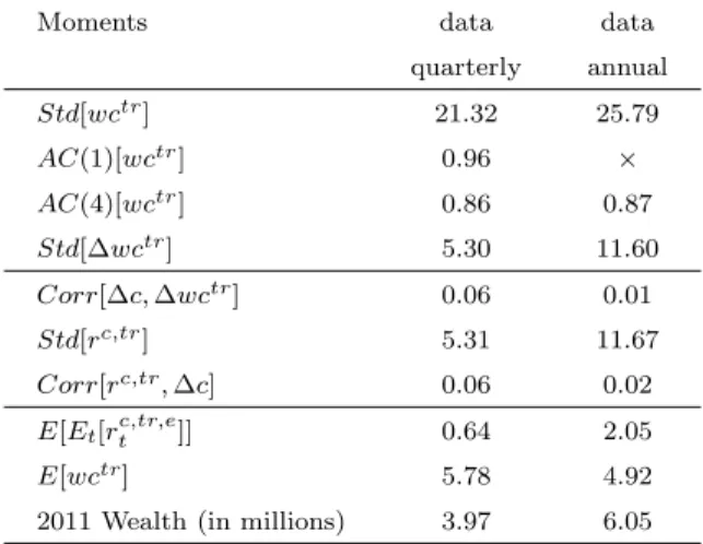
Table 3: Moments of a claim to trend consumption
This table displays unconditional moments for the consumption perpetuity, the claim to deterministically growing aggregate consumption. We report its log wealth-consumption ratiowctr, its first difference ∆wctr, and the log total wealth returnrc,tr.
The last panel reports the time-series average of the conditional consumption risk premium,E[Et[rc,tr,et ]], whererc,tr,edenotes
the expected log return on total wealth in excess of the risk-free rate and corrected for a Jensen term. We report the estimated moments in the data at quarterly and annual frequencies respectively.
Moments data data
quarterly annual Std[wctr] 21.32 25.79 AC(1)[wctr] 0.96 × AC(4)[wctr] 0.86 0.87 Std[∆wctr] 5.30 11.60 Corr[∆c,∆wctr] 0.06 0.01 Std[rc,tr] 5.31 11.67 Corr[rc,tr,∆c] 0.06 0.02 E[Et[rc,tr,et ]] 0.64 2.05 E[wctr] 5.78 4.92
2011 Wealth (in millions) 3.97 6.05
is 6.41% for the dividend claim but only 1.65% for the high-volatility consumption claim. In terms of the dynamics of the risk premia, the high-volatility consumption claim has a correlation of 85% with the standard consumption claim and 83% with the dividend claim. The latter correlation is higher than the 55% correlation between the equity and the actual consumption risk premium. Hence, scaling up the volatility of the consumption claim to that of the dividend claim cannot account for differences in risk premia. If instead, consumption growth were correlated with price-dividend or market return shocks to the same extent as the dividend claim, then naturally the consumption risk premium would inherit the properties of the stock market risk premium.
3.2.4 Wealth creation and destruction
Figure 3 plots the wealth-consumption ratio in levels, alongside NBER recessions (shaded bars). Its dynamics are to a large extent inversely related to the long real yield dynamics in Figure 2. For example, the 5-year real yield increases from 3.5% per annum in 1979.I to 6.9% in 1981.III, while the wealth-consumption ratio falls from 68 to 49. This corresponds
to a loss of $318,000 in real per capita wealth in 2005 dollars, where real per capita wealth is the product of the wealth-consumption ratio and observed real per capita consumption. Similarly, the low-frequency decline of the real yield in the 25 years after 1981 corresponds to a gradual rise in the wealth-consumption ratio. One striking way to see that total wealth behaves differently from equity is to study it during periods of large stock market declines. During the bear markets of 1973.III-1974.IV, 2000.I-2002.IV, and 2007.II-2009.I, the change in U.S. households’ real per capita stock market wealth (including mutual fund holdings) was -46%, -61%, and -65%, respectively. In contrast, real per capita total wealth changed by -12%, +23%, and +11%, respectively.11 Over the full sample, the total wealth return has a correlation of only 27% with the value-weighted real CRSP stock return, while it has a correlation of 94% with realized one-quarter holding period returns on the 5-year nominal government bond.12 Likewise, the quarterly consumption risk premium has a correlation of 55% with the quarterly equity risk premium, lower than the 62% correlation with the quarterly nominal bond risk premium on a 5-year bond.
To show more formally that the consumption claim behaves like a real bond, we compute the discount rate that makes the current wealth-consumption ratio equal to the expected present discounted value of future consumption growth. This is the solid line measured against the left axis of Figure 4. Similarly, we calculate a time series for the discount rate on the dividend claim, the dotted line measured against the right axis. For comparison, we plot the yield on a long-term real bond (50-year) as the dashed line against the right axis. The correlation between the consumption discount rate and the real yield is 99.95%, whereas the correlation of the dividend discount rate and the real yield is only 46%. In addition, the consumption and dividend discount rates only have a correlation of 48%, reinforcing our 11During the Great Recession, total per capita wealth is estimated to have fallen between 2008.II and
2008.IV. In addition to this absolute decline, we argue below that total wealth fell substantially relative to trend wealth over a multi-year period surrounding the Great Recession. Finally, we note that our model might understate the total wealth destruction during the Great Recession if flight-to-safety effects made nominal Treasury yields artificially low.
12
A similarly low correlation of 18% is found between total wealth returns and the Flow of Funds’ measure of the growth rate in real per capita household net worth, a broad measure of financial wealth. The correlation of the total wealth return with the Flow of Funds’ growth rate of real per capita housing wealth is 4%.
Figure 3: The log wealth-consumption ratio in the data Wealth−Consumption ratio Annualized, in levels 1960 1970 1980 1990 2000 2010 40 50 60 70 80 90 100 110
The figure plots exp{wct−log(4)}, wherewct is the quarterly log total wealth to total consumption ratio. The log wealth consumption ratio is given bywct=Ac
0+ (Ac1)′zt. The coefficientsAc0andAc1 satisfy equations (7)-(8).
conclusion that the data suggest a large divergence between the perceived riskiness of a claim to consumption and a claim to dividends in securities markets.
Figure 4: Discount rates on consumption and dividend claim
Percent per year
1960 1970 1980 1990 2000 2010 3 4 5 1960 1970 1980 1990 2000 2010 0 5 10
Percent per year
cons discount rate div discount rate 50−yr real yield
The figure plots the discount rate on a claim to consumption (solid line, measured against the left axis, in percent per year), the discount rate on a claim to dividend growth (dashed line, measured against the right axis, in percent per year), and the yield on a real 50-year bond (dotted line, measured against the right axis, in percent per year). The discount rates are the rates that make the price-dividend ratio equal to the expected present-discounted value of future cash flows, for either the consumption claim or the dividend claim.
A second way of showing that the consumption claim is bond-like is to study yields on consumption strips. We decompose the yield on the period-τ strip into two components. The first component is the yield on a security that pays a certain cash flow (1 + µc)τ.
The underlying security is a real perpetuity with a cash flow that grows at a deterministic consumption growth rate,µc. The second component is the yield on a security that pays off Cτ/C0−(1 +µc)τ; it captures pure consumption cash flow risk. Appendix B.4 shows that
the log price-dividend ratios on the consumption strips are approximately affine in the state, and details how to compute the yield on its two components. In our model, consumption strip yields are mostly comprised of a compensation for variation in real rates (labeled “real bond yield -µc” in Figure B.5), not consumption cash flow risk (labeled “yccr”). Other than
at short horizons, the consumption cash flow risk security has a yield that is approximately zero.
3.2.5 Predictability properties
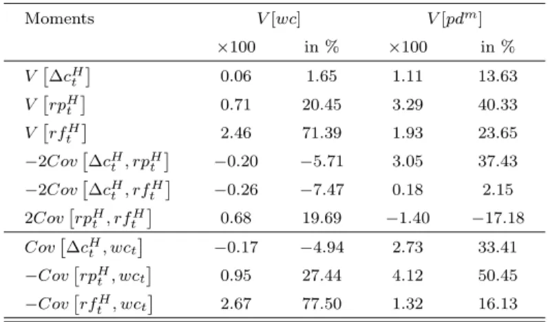
Our analysis so far has focused on unconditional moments of the total wealth return. The conditional moments of total wealth returns are also very different from those of equity returns. The familiar Campbell and Shiller (1988) decomposition for the wealth-consumption ratio shows that the wealth-consumption ratio fluctuates either because it predicts future consumption growth rates (∆cH
t ) or because it predicts future total wealth returns (rtH): V [wct] =Covwct,∆cHt
+Covwct,−rtH
=V ∆cHt +V rtH−2CovrHt ,∆cHt .
The second equality suggests an alternative decomposition into the variance of expected future consumption growth, expected future returns, and their covariance. Finally, it is straightforward to break up Covwct, rHt
into a piece that measures the predictability of future excess returns, and a piece that measures the covariance of wct with future risk-free
covariance terms (See Appendix B). Table 4 reports the complete variance decomposition of the wc and pdm ratios into the three variance terms and the three covariances (top panel)
and into the three covariance terms (bottom panel), under our benchmark calibration. We draw four main empirical conclusions. First, the mild variability of the wc ratio im-plies only mild total wealth return predictability. This is in contrast with the high variability (and predictability) of pdm. Second, 104.9% of the variability in wc is due to covariation
with future total wealth returns, while the remaining -4.9% is due to covariation with future consumption growth. Hence, the wealth-consumption ratio predicts future returns (discount rates), not future consumption growth rates (cash flows). Using the second variance decom-position, the variability of future returns is 111.5%, the variability of future consumption growth is 1.7% and their covariance is -13.2% of the total variance of wc. This variance decomposition is similar to the one for equity. Third, 77.5% of the 104.9% covariance with returns is due to covariance with futurerisk-free rates, and the remaining 27.4% is due to co-variance with futureexcess returns. The wealth-consumption ratio therefore mostly predicts future variation in interest rates, not in risk premia. The exact opposite holds for equity: the bulk of the predictability of the pdm ratio for future stock returns is predictability of excess
returns (50.4% out of 66.5%). Fourth, though modest in both cases, variation in expected future cash-flow growth is more important for the equity claim than for the consumption claim. In sum, the conditional asset pricing moments also reveal interesting differences be-tween equity and total wealth. Again, they point to the strong link bebe-tween the consumption claim return and interest rates.
3.3
Human wealth returns
Our estimates indicate that the bulk of total wealth is human wealth. The human wealth share fluctuates between 86% and 99%, with an average of 92% (see last row of Table 2). Interestingly, Jorgenson and Fraumeni (1989) calculates a similar 90% human wealth share. The average price-dividend ratios on human wealth is slightly above the one on total wealth
Table 4: Variance decomposition wealth-consumption ratio
The first column reports the benchmark wc ratio decomposition; all numbers are multiplied by 100. The second column expresses the numbers of the first column as a percentage of the total variability of thewcratio. The third and fourth columns are the decomposition of thepdmratio in actual values (times 100) and in percent, respectively. For these last two columns, it
is understood that the notation ∆cH
t refers to expected future dividend growth rates.
Moments V[wc] V[pdm] ×100 in % ×100 in % V ∆cH t 0.06 1.65 1.11 13.63 V rpH t 0.71 20.45 3.29 40.33 V rfH t 2.46 71.39 1.93 23.65 −2Cov ∆cH t , rpHt −0.20 −5.71 3.05 37.43 −2Cov ∆cH t , rftH −0.26 −7.47 0.18 2.15 2Cov rpH t , rftH 0.68 19.69 −1.40 −17.18 Cov ∆cH t , wct −0.17 −4.94 2.73 33.41 −Cov rpH t , wct 0.95 27.44 4.12 50.45 −Cov rfH t , wct 2.67 77.50 1.32 16.13
(93 vs. 83 in annual levels). The risk premium on human wealth is very similar to the one for total wealth (2.31 vs. 2.38% per year). The price-dividend ratios and risk premia on human wealth and total wealth have a 99.87% (99.95%) correlation.
Existing approaches to measuring total wealth make ad hoc assumptions about expected human wealth returns. Campbell (1996) assumes that expected human wealth returns are equal to expected returns on financial assets. This is a natural benchmark when financial wealth is a claim to a constant fraction of aggregate consumption. Shiller (1995) models a constant discount rate on human wealth. Jagannathan and Wang (1996) assume that expected returns on human wealth equal the expected labor income growth rate; the resulting price-dividend ratio on human wealth is constant. The construction of cay in Lettau and Ludvigson (2001a) makes that same assumption. Our approach avoids having to make arbitrary assumptions on unobserved human wealth returns.13
Our estimation results indicate that expected excess human wealth returns have an annual volatility of 2.9%. This is substantially higher than the volatility of expected labor income growth (0.6%), but lower than that of the expected excess returns on equity (3.3%). Lastly, 13These models can be thought of as special cases of ours, imposing additional restrictions on the market