LUND UNIVERSITY SCHOOL OF ECONOMICS AND MANAGEMENT
A Spatio-Temporal Study of
Regional House Prices in Sweden
A thesis about interregional house prices in the Swedish market
Marc Montelius ⦁ Markus Niemelä
Abstract
This paper uses a recently developed methodology to investigate the spatial and temporal diffusion patterns of a shock to the regional house markets in Sweden. We model the change in regional house prices such that they are allowed to be contemporaneously affected by price changes in the dominant region – Stockholm - as well as being allowed to be subject to a cointegrated relationship with its neighboring regions and Stockholm. Own lagged price effects as well as neighboring lag effects are also considered. We find that shocks to the Stockholm housing market contemporaneously affects Malmo and Gothenburg the most, leading us to believe that the relationship between regional housing markets in Sweden best can be explained by homogenous economic conditions within the regions.
Keywords: House prices, ripple effect, interregional dependence, spatial & temporal diffusion
Department of Economics Supervisor - Joakim Westerlund First Year Master Thesis
1
1.
Introduction
House prices in Sweden have been at the center of attention for quite some time due to the seemingly never ending surge in prices. But how are prices on the housing market decided? Is it according to the neoclassical life-cycle framework, with demand and supply as the fundamental deciders, or is it perhaps more to the story? In recent years, economists has laid out the theory of temporal and spatial-dependency of house prices; that the regional markets are not independent markets, but part of a dynamic system of markets where spillover-effects and temporal adjustments are important contributors when it comes to modelling house prices.
The pattern of which house prices spread inter-regionally is often referred to as “the ripple effect”, and evidence of this has been found mainly in the UK, where several studies have concluded that price changes start in the South-East region and then gradually spreads to the rest of the country. There is however little consensus amongst researchers on how to best model the spatial and temporal patterns, as new models are continuously being proposed.
One of the main issues regarding modeling spatial patterns arises from the definition of proximity. One commonly used approach is to use the geographical distance between regions. There is however some who instead argue that the measurement of proximity instead should depend on other factors, such as integrated industrial-, labor- or financial markets. There are many unanswered questions in the field of spatial diffusion of prices, and for temporal and spatial diffusion the unexplored territory is even greater.
Understanding what drives prices and house prices in this context is crucial in order to have well-functioning markets and for the regional distribution of wealth. Housing is arguably one of the most important assets of any household in today’s society and the development of prices has a direct effect on the living situation for individuals and families.
We will in this paper use a recently developed methodology in order to estimate the short- and long-run dynamics of regional house prices in Sweden to see if we can find a similar ripple effect on the Swedish market as has been found in other countries. This is done by first checking for cointegration amongst the regional markets, where we by
2 conducting several tests find indications towards that several of the sub-markets are in fact interdependent and must therefore be treated as such. We find, after testing for significant effects and weak exogeneity that Stockholm can be seen as a dominant region regarding house prices in Sweden and that shocks in Stockholm will affect remaining regions. We also find certain indications that the ripple effect might be stronger over space than over time; the shock tends to die out faster over time than it does over distance.
The remaining part of this paper is structured as follows; in section 2 we present a brief overview of the existing literature with a focus on the relevant research for this paper. Section 3 gives a short theoretical background on determinants of house prices and the interregional dependencies. In section 4 we describe the data used for this paper and its properties before moving on to section 5 where we describe the methodology we use to estimate our model and conduct our tests. Section 6 presents our main results and briefly discusses them, and section 7 then concludes the paper by summarizing our findings.
2.
Literature
review
A large amount of studies have been made on analyzing house prices. Previous research has tried to analyze the relationship between national house prices and various macroeconomic variables1, and others have studied the effect of monetary policy on house price movements2. More recently, many researches have tried to analyze regional data instead of national. Since regional house price data is generally richer and contain more information about the determinants of house prices, these models could have some advantages over models with national data.
The long-rung relationships between regional house prices have for a long time been analyzed and have set the basis for further research. The best known, and early written papers that examine cointegrating relationships of house prices between regions are
1 For a recent Swedish example see Gustafsson et al. (2016). The authors to this paper try to analyze the
macroeconomic effects of a decline in housing prices in Sweden using a Bayesian VAR model.
2 See for example Yang et al. (2010). This study measures the effects of monetary policy on regional
3 those of Alexander et al. (1994) and MacDonald et al. (1993). Both these papers show the existence of long-run relationships between regional house prices in England. One of the first studies that considered the spatial diffusion of house prices is due to Can (1990), in which he studied what he called “neighborhood dynamics”. Can (1990) use a hedonic house price model, where house prices include both spatial parametric drift and spatial spillover effects. Later studies moved on by analyzing the prices over time as well. A study from the Netherlands by Dijk et al. (2007) incorporates both dimensions. Their models allows for cointegration, stochastic trends and cross-equation correlation. Their paper manages to capture the ripple effect in which shocks from one region would spread to other regions. Similar papers were also made by Holly et al. (2010 & 2011).
A number of empirical studies have analyzed regional house price dynamics, where it is assumed that house price movements diffuse from one economic center (often the largest city in a country) to the surrounding regions, see e.g. Meen (1996). Papers by Munro et al. (1996) and Giussani et al. (1991) try to model the ripple effect for British housing data. They do this by including house prices for London as regressor in house price equations for other regions in England.
Although most previous research show that the largest city Granger-cause price movements in other regions, some research show that there are cases where smaller regions dominate larger ones. One example of this can be seen in a paper by Oikarinen (2005). His results show that changes in housing price in the suburbs of Helsinki Granger-cause changes in the city center. The larger Helsinki metropolitan area does however Granger-causes the other regions in Finland.
In a recent study from Belgium, Helgers et al. (2016) look at the ripple effect and are particularly interested in the effects due to linguistic borders. Like the other papers they first try to determine the dominating region and then look at the cointegrating relationships towards the other regions. The authors also run a generalized spatio-temporal impulse response function and are thus able to provide evidence for the existence of the ripple effect.
There are also studies of Sweden. One of the very first studies is that of Berg (2002). In his paper, Berg finds that the Stockholm region Granger-causes all other regions in
4 Sweden, which draws the conclusion that the Stockholm region can be seen as the dominating region. Berg also finds that many macro variables Granger-cause house prices in the Stockholm region, and therefore, indirect house prices in all other regions. The study does however not mention the possible existence of long-run dynamics. In a more recent study, Yang et al. (2016) analyze regional house prices in Sweden but with a slightly different approach. They try to quantify the relative importance of shocks in determining regional house prices. By using a multivariate shock persistence method they can look at the effect from a change in fundamental macroeconomic variables and the effect of regional spillovers at the same time. In their models they define Stockholm, Gothenburg and Malmo as the “core” regions and look at the spillover effects towards Sweden’s local labor markets which are aggregated into six regions. The results are that there is a long-run temporal and spatial diffusion between the regions. The results and method from this thesis can be used to analyze the effect of a shock from i.e. a national economy or policy in regional diffusion.
In a paper by Holly et al. (2011) the authors model the temporal and spatial diffusion of shocks in non-stationary dynamic systems. They look at regional house prices in the UK with London as a dominant region. Their results show that house prices in other regions respond directly to shocks in the dominant region and that the shock is intensified both by the inner dynamic of each region and by connections with neighboring regions. They also modify an impulse response analysis where they show that the effects of a shock decline more slowly along the geographical dimension as compared to the decline over time. The model used in this paper can be applied to any other market in which a dominant region is found. The aim of this thesis is therefore to see if similar results could be seen in Sweden.
3.
Theoretical framework
The idea of a spatial relationship in regional housing markets can be taken from the First Law of Geography: “everything is related to everything else, but near things are more related than distant things” – Tobler (1970).
Most work on housing economics has its roots in the life-cycle theory of household behavior and consumption. It states that all households attempt to maximize its expected
5 utility within the limits of their household budget. By lending and borrowing, agents are not constrained by their current income and can take advantages of future expected opportunities. The theory can also be summarized down to a model which shows how the rate of return from housing investment depends on a number of variables: income, capital gain, depreciation of housing stock, tax rate, mortgage rate, interest rate, construction costs and inflation rate3. A similar model is presented by Muellbauer and Murphy (1994), in which they write the invert demand function with the real price of housing as a function of similar variables. As rational agents would like to maximize their expected utility, it is assumed that agents also try to make the optimal decisions when it comes to investment in housing. This in turn will affect demand and supply in the housing market. The life-cycle theory can however be criticized, as most macroeconomic models, for its assumptions on perfect information, rational agents and zero transaction costs.
Furthermore, the rather basic macroeconomic model also does not take into account the spatial dimensions that should be necessary for analyzing regional house prices. In fact, this issue is often entirely ignored by the macroeconomic literature4. Regional markets are not independent economic units; they should be seen as sub-markets within the housing market. Regional housing markets have temporal dimensions as well as spatial ones; they could depend on previous price movements and spillover effects from neighboring regions. Overlooking the spatial dimension could lead to biased estimations in standard statistical and econometric analysis of house prices. This is something that has led to the development of spatial econometrics in recent years.
The level of house prices can vary greatly between different regions within the same country. It is very common that house prices in larger metropolitan areas greatly exceed those in the rural areas of the country. Although there should not be any lead-lag relationships between assets5 in perfect capital markets, many factors might account for lagged relationships in price movements. There are many reasons for house price movements in a larger region to lead prices in other regions. The primary theory
3 For a full description of the formal model, see Meen (1990), or a summarized version in Meen (1999).
Note however that this model is based out of standard macroeconomic theory and can be found in various macroeconomic textbooks.
4 The concern that this was not included, and that there was an independently approach to analyzing
housing markets (micro vs. macro) was written by McAvinchey & Maclennan (1982).
5
6 suggests that business cycles are a major factor in determining housing prices6; and as business cycles tend to first hit a dominant economic region, due to the high amount of financial- institutions and services in those regions, one could assume that shocks spread to the neighboring regions with some lag7.
Another argument for a lead-lag relationship between regions is information asymmetry. In larger or more densely populated regions one could assume that the amount and availability of information on recent macroeconomic shocks will be greater, therefore giving agents in these regions some advantages to adjusting to those kinds of shocks8. It should therefore take some time before agents in other regions adjust to changes.
As suggested by Meen (1999) the observed pattern of the ripple effect could also be explained by migration, equity transfer and spatial arbitrage in the determinants of house prices. Meen argues that if house prices differ between regions then households are expected to migrate to the regions where prices are lower; this would lead to a smoothening of regional prices over time9. The second argument of equity transfer10 is closely related to migration and suggests that agents in regions with higher prices would have greater buying power, leading to higher prices in the other regions if these agents would want to move.
Furthermore, due to information asymmetry (as discussed above) and search costs one could assume that fully efficient arbitrage opportunities will not be possible. The arbitrages of capital will instead follow a gradient transfer process. The last argument also implies that there could be different patterns of house prices even if there are no spatial links between regions. For instance, different regional growth patterns could explain why house prices in some regions grow before other regions11.
Although there are many theories that support the existence of the ripple effect less is said about the direction, timing and magnitude of the effect. How long should we expect
6 In these business cycles a positive shock would lead to an increasing number of jobs and a higher level
of income. These, plus many additional factors, would lead to an increase in the demand and therefore price of housing.
7 One could of course also note that some shocks, like a sudden change in the level of real interest rates,
will affect all regions in a country at the same time.
8
These ideas were introduced by Grossman et al. (1976) and later supported by Clapp et al. (1995).
9 This idea is also discussed by Alexander & Barrow (1994) and Giussani & Hadjimatheou (1991a). 10 This idea is built on work by Stein (1995) and Muellbauer & Murphy (1994).
11 Further explained and discussed by Muellbauer & Murphy (1994) and Giussani & Hadjimatheou
7 the ideas of equity transfer and spatial arbitrage to matter for the diffusion of price changes between regions? A macro shock to a dominant region could spread with some lag to other regions, but it remains unclear what types of regions that are most affected and why. Due to proximity in terms of transportation opportunities, one theory suggests that regions that are geographically near should be affected more. Proximity however, does not have to be limited to proximity over space. One could also look at other measures of distance, such as financial, economic or social12. For instance two major cities in a country, with closely linked financial markets, might have more connected housing prices than a rural neighboring region, even though the geographical distance is much larger. It is also clear that the structural differences in regional housing markets will determine the effect; different tax-rates, regional demand and supply are some factors that are important to consider.
4.
Data
The house price indices used in this paper are the price development of the existing stock of one- or two-dwelling buildings for permanent living collected and constructed by Statistics Sweden13. The indices covers the period between 1986q1 up to 2016q4 (T=124) and are presented in Figure 2 and in Figure 314.
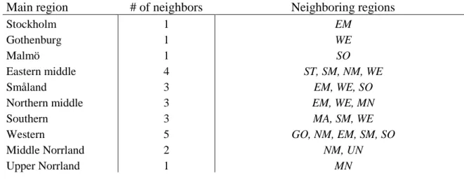
There are 10 different regions used in this paper, which is illustrated in Figure 1 and Table 1. The regional definition used in this paper is NUTS 2, which is the regional selection used within the European Union for the reporting of statistics15.
12 See for example Conley (1999), Pesaran, Schuermann and Weiner (2004). 13 See www.scb.se for more information regarding the construction of the indices. 14
Due to the index construction, house price indices as a source for empirical analysis have been criticized; see, Can et al (1997), Himmelberg et al (2005) and McCarthy et al (2004). Indices are however one of the best and readily available datasets to use for researchers; see Wheelock (2006) and Harter-Dreiman (2003).
15
8 Figure 1 – Regions and their borders
Table 1 - Regions, abbreviations, sub-regions and list of neighbors
Main region Abbrev. Included sub-regions
Stockholm ST Stockholm
Gothenburg GO Gothenburg
Malmö MA Malmö
Eastern middle EM Örebro, Östergötland, Södermanland, Uppsala, Västmanland
Småland SM Gotland, Jönköping, Kalmar, Kronoberg
Northern middle NM Dalarna, Gävleborg, Värmland
Southern SO Blekinge, Skåne
Western WE Halland, Västergötland
Middle Norrland MN Jämtland, Västernorrland
9 Main region # of neighbors Neighboring regions
Stockholm 1 EM
Gothenburg 1 WE
Malmö 1 SO
Eastern middle 4 ST, SM, NM, WE
Småland 3 EM, WE, SO
Northern middle 3 EM, WE, MN
Southern 3 MA, SM, WE
Western 5 GO, NM, EM, SM, SO
Middle Norrland 2 NM, UN
Upper Norrland 1 MN
There is a clear upward trend in the house prices for all regions. We can however see that some regions, mainly the larger city regions, have grown at a higher rate than the others, especially since the beginning of the new millennia. This could possibly be explained by the migration from smaller municipalities to the greater cities and the shortage of housing stock in said areas due to lack of space to build. Descriptive statistics for the change in each region is presented in Table 2. We can clearly see that the mean change in housing prices is highest in the largest cities, and they also have the largest standard deviations, partly explained by the inability to quickly adjust the housing stock to account for a rapid urbanization16.
Table 2 - Descriptive statistics of change in house prices for all regions in Sweden
Region Mean Std. Dev. Obs
ST 7,8 12,9 123 GO 6,7 11,6 123 MA 7,0 13,3 123 EM 4,3 6,7 123 WE 5,3 8,6 123 SM 3,8 7,2 123 SO 5,3 9,3 123 NM 3,1 6,6 123 MN 2,4 7,1 123 UN 2,8 7,8 123 16
10 0 200 400 600 800 1000 1200 1986 1991 1996 2001 2006 2011 2016
Figure 2 - House price indices in Swedish regions (1986Q1 - 2016Q4)
ST GO MA WE SO EM SM NM UN MN -40,00 -30,00 -20,00 -10,00 0,00 10,00 20,00 30,00 40,00 50,00 60,00 1986 1991 1996 2001 2006 2011 2016
Figure 3 - Change in house price indices in Swedish regions (1986Q1 - 2016Q4)
∆ST ∆GO ∆MA ∆WE ∆SO
11 House prices and house price indices are often assumed to be first-difference stationary and several earlier studies have concluded this to be the case, see e.g. Barot & Yang (2002), Oikarinen (2005), Turner & Yang (2016) and Berg (2002). From the results of the Augmented Dickey-Fuller (ADF) test we can conclude that all indices are non-stationary in levels but only some are non-stationary in first-differences. Further tests do however confirm that all indices are stationary in differences as well17.
Finally, for the use of GDP-data we use seasonally adjusted GDP at constant prices also retrieved from Statistics Sweden.
5.
Methodology
Suppose we are interested in the diffusion of Swedish house prices over both time and space where the regions are denoted by 𝑖𝑖= 0,1,2, . . ,𝑁𝑁 and time by 𝑡𝑡 = 1,2, . . ,𝑇𝑇 and that we here believe that there exist a dominant region, 0, such that shocks to region 0 spread instantaneously to all other regions. Shocks to the remaining regions however, have little or no immediate effect on region 0. Lagged effects on region 0 of shocks on other regions are allowed for. Following the notation of Holly et al. (2011), we can write a first order linear error correction specification for region 0 as:
∆𝑝𝑝0𝑡𝑡 =𝜃𝜃0𝑠𝑠�𝑝𝑝0,𝑡𝑡−1− 𝑝𝑝0,𝑡𝑡−1−𝑠𝑠 �+𝛼𝛼0+𝛼𝛼01∆𝑝𝑝0,𝑡𝑡−1+𝑏𝑏01∆𝑝𝑝0,𝑡𝑡−1−𝑠𝑠 +𝛾𝛾0∆𝐺𝐺𝐺𝐺𝐺𝐺𝑡𝑡+𝜀𝜀0𝑡𝑡 and for the following regions we get the following specification:
∆𝑝𝑝𝑖𝑖𝑡𝑡 =𝜃𝜃𝑖𝑖𝑠𝑠�𝑝𝑝𝑖𝑖,𝑡𝑡−1− 𝑝𝑝𝑖𝑖,𝑡𝑡−1−𝑠𝑠 �+∅𝑖𝑖0�𝑝𝑝𝑖𝑖,𝑡𝑡−1− 𝑝𝑝0,𝑡𝑡−1�+𝛼𝛼𝑖𝑖+𝛼𝛼𝑖𝑖1∆𝑝𝑝𝑖𝑖,𝑡𝑡−1+𝑏𝑏𝑖𝑖1∆𝑝𝑝𝑖𝑖,𝑡𝑡−1−𝑠𝑠 + 𝑐𝑐𝑖𝑖0∆𝑝𝑝0𝑡𝑡 + 𝑑𝑑𝑖𝑖1∆𝑝𝑝0,𝑡𝑡−1+𝛾𝛾𝑖𝑖∆𝐺𝐺𝐺𝐺𝐺𝐺𝑡𝑡 + 𝜀𝜀𝑖𝑖𝑡𝑡
where 𝑝𝑝𝑖𝑖𝑡𝑡−𝑠𝑠 denotes the spatial variable for each region and is in this paper set in advance as a simple average of the price levels of the neighboring regions such that:
𝑝𝑝𝑖𝑖𝑡𝑡−𝑠𝑠=∑𝑁𝑁𝑖𝑖=0𝑠𝑠𝑖𝑖𝑖𝑖𝑝𝑝𝑖𝑖𝑡𝑡 where ∑𝑁𝑁𝑖𝑖=0𝑠𝑠𝑖𝑖𝑖𝑖= 1 for i = 0, 1, 2,..,N
in this paper we use the definition that two regions are neighbors if they share a border, 𝑠𝑠𝑖𝑖𝑖𝑖 is therefore calculated as 𝑛𝑛1𝑖𝑖 in the case of i and j sharing a border and 0 if they do
17
12 not. There is much research on the selection of proximity measurement18, for simplicity we have decided to limit our analysis to use the above mentioned contiguity measurement, however one could also argue that industrial connections and migration would be important factors in the measurement.
Since there is the possibility that house price changes are the result of macroeconomic developments we also add the change in GDP (∆𝐺𝐺𝐺𝐺𝐺𝐺𝑡𝑡) to our regressions, following the methodology of Buyst & Helgers (2016).
The price equations are allowed to be of an error correction specification, although this is not necessarily the case as the specification depends on whether the series are cointegrated. In our specification we allow for the dominant region to be cointegrated with its neighbors and the remaining regions to be cointegrated with both its neighbors and with the dominant region. 𝜃𝜃𝑖𝑖𝑠𝑠 denotes the error correction coefficients towards the neighboring regions and ∅𝑖𝑖0 is the error correction coefficient towards the dominant region. These coefficients are assumed to be significant if long-run relationships between the regions are found, i.e. if the regions are cointegrated.
Testing for cointegration can be done either using a pairwise approach19 or jointly by setting up a VAR model including all regions. As we have assumed that region 0 can be taken as a dominant region and is allowed to be cointegrated with all other regions we will set up a bivariate VAR specification in levelswith 𝑝𝑝0𝑡𝑡 and 𝑝𝑝𝑖𝑖𝑡𝑡 for all i. Testing for cointegration is then carried out using the test developed by Johansen (1991).
Continuing following the specification of Holly et al. (2011), we can see that the included contemporaneous effect on region i from region 0, and the lack of a contemporaneous local effect on region 0, implicitly means that, conditional on region 0’s price variable and the lagged effects the shocks are independently distributed throughout the regions. This means that ∆𝑝𝑝0𝑡𝑡 is assumed to be weakly exogenous in the price equation for the remaining regions. This is tested by following the procedure laid out by Wu (1973), where the residuals for the dominant region (𝜇𝜇), calculated using OLS, are included as a separate regressor in the price equation for the remaining regions:
18 See for example Holly et al. (2011) and Brady (2013) for more discussion on different approaches. 19
13
∆𝑝𝑝𝑖𝑖𝑡𝑡 =𝜃𝜃𝑖𝑖𝑠𝑠�𝑝𝑝𝑖𝑖,𝑡𝑡−1− 𝑝𝑝𝑖𝑖,𝑡𝑡−1−𝑠𝑠 �+∅𝑖𝑖0�𝑝𝑝𝑖𝑖,𝑡𝑡−1− 𝑝𝑝0,𝑡𝑡−1�+𝛼𝛼𝑖𝑖+𝛼𝛼𝑖𝑖1∆𝑝𝑝𝑖𝑖,𝑡𝑡−1+𝑏𝑏𝑖𝑖1∆𝑝𝑝𝑖𝑖,𝑡𝑡−1−𝑠𝑠 +𝑐𝑐𝑖𝑖0∆𝑝𝑝0𝑡𝑡+ 𝑑𝑑𝑖𝑖1∆𝑝𝑝0,𝑡𝑡−1+𝜗𝜗𝑖𝑖𝜇𝜇+𝜖𝜖𝑖𝑖𝑡𝑡
then a simple Wald-Test is used to calculate the t-statistic of H0: 𝜗𝜗= 0.
One way of analyzing the connection between regions is to use the Granger-causality test provided by Granger (1969). For our paper, the Granger-causality test can be used as a method to further investigate if the changes in house prices in region 0 can be used to “explain” the price changes in other regions in addition to its own changes; if ∆𝑝𝑝0𝑡𝑡 can “explain” ∆𝑝𝑝𝑖𝑖𝑡𝑡 . We can describe the test in the following way for region 0 and region i:
∆𝑝𝑝0𝑡𝑡 =𝜌𝜌0+� 𝛼𝛼𝑖𝑖∆𝑝𝑝0,𝑡𝑡−𝑖𝑖 𝑘𝑘 𝑖𝑖=1 +� 𝛽𝛽𝑖𝑖 𝑘𝑘 𝑖𝑖=1 ∆𝑝𝑝𝑖𝑖,𝑡𝑡−𝑖𝑖+𝜀𝜀𝑡𝑡
where we estimate 𝜌𝜌, 𝛼𝛼, 𝛽𝛽 for a given lag. Testing H0:𝛽𝛽1 = 𝛽𝛽2= ⋯= 𝛽𝛽𝑘𝑘= 0, and failing to reject indicates that 𝑝𝑝𝑖𝑖 does not Granger-cause 𝑝𝑝0.
Weak exogeneity and the Granger-causality test will give us indications on the suitability of our choice of dominant region. In addition to these tests, we will in accordance with Holly et al. (2011) and Buyst & Helgers (2016), estimate the appropriate Cointegrating Bivariate VAR model of regional house prices, where we assume a dominant region, and estimate the error correction coefficients between the dominant region and region i, in order to give us indications on the long-run dynamics. Even though the price equations can, and will, be estimated separately using OLS, in order to simulate the model we have a system of equations that needs to be solved together. Following Holly et al. (2011) and Buyst & Helgers (2016), we choose a Generalized Impulse Response Function (GIRF)20, to analyze how shocks are spread throughout the regions over time and space. By using a generalized impulse response function instead of the more conventional orthogonalized impulse response we allow for contemporaneous correlations between regions i and j where i, j = 1,2…N. The generalized impulse response function is also invariant to the ordering of the variables in the VAR-model
20
14
6.
Results
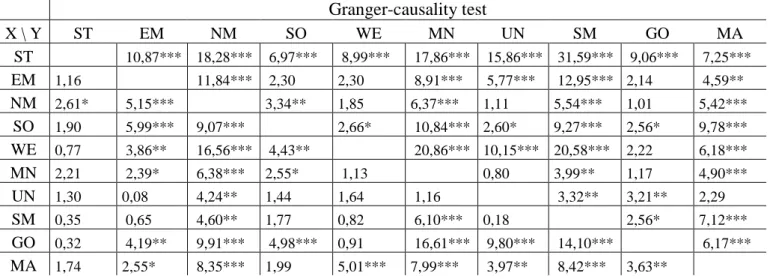
The result of the analysis indicates that the Swedish regional house price indices are highly correlated, both in levels and in differences. However, since correlation does not necessarily imply causation we begin by applying the Granger-causality test to see whether or not changes in house prices in one region can be used to explain the changes in other regions in addition to their own changes. As we can see in Table 5, the null-hypothesis that Stockholm does not Granger-cause another region can be rejected for all regions at the 1% level. We can also see that the null-hypothesis that a region does not Granger-cause Stockholm cannot be rejected for any of the regions. The results remain roughly the same, independently on the number of lags chosen21. This strengthens our hypothesis that Stockholm can be seen as a dominant region22.
Table 5 - Granger-causality test statistics of house price changes between the different regions
Granger-causality test X \ Y ST EM NM SO WE MN UN SM GO MA ST 10,87*** 18,28*** 6,97*** 8,99*** 17,86*** 15,86*** 31,59*** 9,06*** 7,25*** EM 1,16 11,84*** 2,30 2,30 8,91*** 5,77*** 12,95*** 2,14 4,59** NM 2,61* 5,15*** 3,34** 1,85 6,37*** 1,11 5,54*** 1,01 5,42*** SO 1,90 5,99*** 9,07*** 2,66* 10,84*** 2,60* 9,27*** 2,56* 9,78*** WE 0,77 3,86** 16,56*** 4,43** 20,86*** 10,15*** 20,58*** 2,22 6,18*** MN 2,21 2,39* 6,38*** 2,55* 1,13 0,80 3,99** 1,17 4,90*** UN 1,30 0,08 4,24** 1,44 1,64 1,16 3,32** 3,21** 2,29 SM 0,35 0,65 4,60** 1,77 0,82 6,10*** 0,18 2,56* 7,12*** GO 0,32 4,19** 9,91*** 4,98*** 0,91 16,61*** 9,80*** 14,10*** 6,17*** MA 1,74 2,55* 8,35*** 1,99 5,01*** 7,99*** 3,97** 8,42*** 3,63** The test is conducted by seeing if the null-hypothesis X does not Granger-cause Y, can be rejected or not. *** signifies that the test rejects the null at the 1% level, ** at the 5% level and * at the 10% level.
To examine whether or not changes in Stockholm house prices are weakly exogenous to the movement of house prices in other regions we use the Wu-Hausman test statistics. The result of the test is shown in Table 6. It shows that the null-hypothesis that price
21 We test for lags of one quarter, six months and a year. 22
15 changes in Stockholm are weakly exogenous for house prices in all other regions, cannot be rejected for any region except for Smaland. Since it is possible that there may be other forms of pair-wise dominance, we also allow each region in turn to be the dominant region. As we can see in the same table, there are in fact many other regions for which the null cannot be rejected for any other region (NM, MN, SM, MA), and some regions for which we can only reject the null for one other region (EM, WE, GO). According to this test, these regions could also be potential candidates for the choice of dominant region23.
Table 6 - Wu-Hausman statistics for testing the exogeneity of house prices of the assumed dominant region
Assumed Dominant Region
ST EM NM SO WE MN UN SM GO MA ST - 0,29 2,01** -0,87 0,55 -5,17*** -0,73 2,64*** 0,99 EM 1,47 - 0,89 3,92*** -1,79* -0,45 -4,89*** -0,62 1,22 -1,34 NM -1,16 -0,19 - 2,27** 0,37 0,22 0,78 0,42 -0,68 -1,21 SO -0,32 0,25 0,93 - 0,17 -0,37 -2,67*** 1,66 -0,16 WE 0,57 -0,41 0,04 0,13 - -0,07 -3,19*** -1,28 1,79* MN -1,92 -1,57 -0,86 -0,23 0,58 - -1,35 -0,89 -1,43 UN -1,18 1,33 -1,64 -1,54 2,03** - -1,65 0,33 0,85 SM -2,03** -2,33** 0,62 1,98* -1,06 -1,43 -1,12 - -1,53 0,96 GO 0,87 0,35 0,26 -0,07 -0,63 -1,84* -0,25 - 1,26 MA -0,71 -0,92 -0,78 -0,06 -1,56 -3,52*** 0,63 1,66 - Each region is in turn assumed to be the dominant region (top row), and is then tested for against the other regions (first column). *** signifies that the test rejects the null at the 1% level, ** at the 5% level and * at the 10% level. Empty cells represents missing values due to the specification of the spatial variable.
Table 7 contains the trace statistics calculated using the above mentioned Johansen method. Using our methodology and assuming that Stockholm is the dominant housing price region we present the statistics of a pairwise test between Stockholm and region i taken from a Bivariate VAR model. We find that the null hypothesis of no cointegration between Stockholm and region i can be rejected for four of the nine other regions. It appears from the pairwise-test that the Stockholm housing market tends to be cointegrated mainly with regions that are geographically close to it, with the exception of Upper Norrland.
23
16 Table 7 – Pairwise-trace cointegration test
Cointegration test Test 1 Test 2 EM 21,82* 2,26 NM 23,87* 0,93 SO 7,18 1,61 WE 11,19 2,08 MN 14,27 0,31 UN 9,4 4,07* SM 18,45* 2,24 GO 9,75 2,83 MA 7,67 1,31
Tests if there is a cointegrating relationship between Stockholm and the other regions. More precisely it tests of over-identifying restrictions in Bivariate VAR models of house price indices of Stockholm and the other regions. The first column test the null of r = 0 against the hypothesis of r ≥ 1. The second column tests the null of r ≤ 1 against the hypothesis of r = 2. * signifies that the test rejects the null at the 5% level.
We also conduct a joint-test for cointegration using Johansen’s method were we find that the test statistics indicate that the regional house markets tend to be restored in seven cointegrations in the regions. The results are presented in Table 8.
Table 8 - Joint-test for cointegration between all regional house price indices
Unrestricted Cointegration Rank Test (Trace)
Hypothesized No. of CE(s) Eigenvalue Trace Statistic 0.05 Critical Value Prob.** None * 0,49 390,51 273,19 0,00 At most 1 * 0,41 308,96 228,30 0,00 At most 2 * 0,37 245,33 187,47 0,00 At most 3 * 0,34 188,97 150,56 0,00 At most 4 * 0,27 138,95 117,71 0,00 At most 5 * 0,25 100,96 88,80 0,01 At most 6 * 0,19 66,95 63,88 0,03 At most 7 0,14 41,08 42,92 0,08 At most 8 0,12 22,87 25,87 0,11 At most 9 0,06 7,18 12,52 0,33
The test is based on Johansen’s method with the data in levels, lag-length of two (according to the Schwarz Bayesian Criterion) and includes both an intercept and trend.
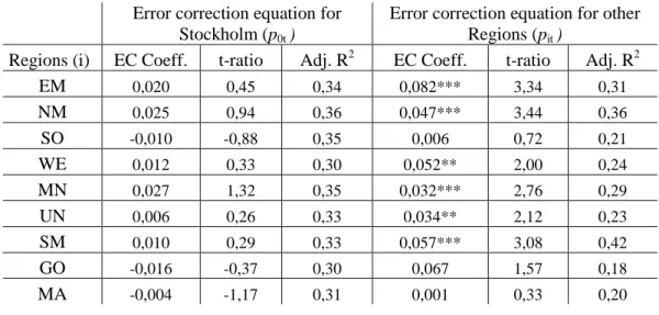
17 We then estimate a Cointegrating Bivariate VAR model to get estimates of the error-correction terms in each pairwise combination of Stockholm and the remaining regions. The results of these are presented in Table 9 where the error-correction term for the Stockholm price equation is presented in the left hand column and the region i’s term is presented in the right hand column. It appears that Stockholm house prices are long-run forcing six out of nine regions, with the exceptions being the Southern region, Malmo and Gothenburg. The results also show no significant effect of the error correction term in the equation of Stockholm house prices. These results are in line with the assumption we made regarding using Stockholm as the dominant region.
Table 9 - Error correction coefficients in Cointegrating Bivariate VAR models of house prices of Stockholm and the other regions
Error correction equation for Stockholm (p0t )
Error correction equation for other Regions (pit )
Regions (i) EC Coeff. t-ratio Adj. R2 EC Coeff. t-ratio Adj. R2
EM 0,020 0,45 0,34 0,082*** 3,34 0,31 NM 0,025 0,94 0,36 0,047*** 3,44 0,36 SO -0,010 -0,88 0,35 0,006 0,72 0,21 WE 0,012 0,33 0,30 0,052** 2,00 0,24 MN 0,027 1,32 0,35 0,032*** 2,76 0,29 UN 0,006 0,26 0,33 0,034** 2,12 0,23 SM 0,010 0,29 0,33 0,057*** 3,08 0,42 GO -0,016 -0,37 0,30 0,067 1,57 0,18 MA -0,004 -1,17 0,31 0,001 0,33 0,20
This tests the null-hypothesis of no error correction effect. *** signifies that the test rejects the null at the 1% level, ** at the 5% level and * at the 10% level.
6.1 Regional House Price Estimates
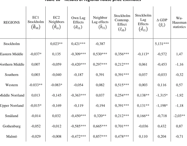
The results of the estimates of the regional house prices where we assume Stockholm to be the dominant region and allowing for error-correction towards Stockholm and neighboring regions is presented in Table 10. The price equations are estimated using OLS, which will yield consistent estimates as long as the Stockholm house prices are weakly exogenous. We estimate all models using a one period lag.
18 We find that the error-correction term for long-run convergence with the dominant region is statistically significant for only one of the regions (Western). We also find that the error-correction term towards neighboring regions is only significant for Stockholm. In the equations for the remaining eight regions, neither error-correction term is significant. This result is somewhat surprising given our cointegration and Granger-causality results. The results from these test indicates that there should be a statistically significant long-run relationship between some of the regions. The reason for this outcome is difficult to interpret and could be the result of several factors. The regions could for instance have other error-correction properties that our simplified model is unable to capture.
Table 10 – Results of regional house price estimates
Significant values are shown by: *** at the 1% level, ** at the 5% level and * at the 10% level. REGIONS EC1 Stockholm �∅�𝑖𝑖0� EC2 Neighbors �𝜃𝜃�𝑖𝑖𝑠𝑠� Own Lag Effects (𝛼𝛼�𝑖𝑖1) �𝑏𝑏�𝑖𝑖1� Neighbor Lag effects Stockholm Contemp. Effect (𝑐𝑐̂𝑖𝑖0) Stockholm Lag Effects �𝑑𝑑̂𝑖𝑖1� ∆ GDP (𝛾𝛾�𝑖𝑖) Wu-Hausman statistics Stockholm 0,023** 0,421*** -0,387 5,131*** Eastern Middle -0,037* 0,135 -0,309*** 0,530*** 0,356*** -0,113* -0,572 1,47 Northern Middle 0,007 -0,059 -0,420*** 0,297*** 0,212*** 0,061 -0,453 -1,16 Southern 0,003 -0,040 -0,187 0,391 0,391*** 0,037 -0,033 -0,32 Western -0.033** -0.083* -0,054 0,082 0,515*** 0,003 0,116 0,57 Middle Norrland 0,013 -0,145 -0,363*** 0,037 0,254*** 0,138** -1,315* -1,92 Upper Norrland -0,015* -0,169 -0,119 -0,194 0,391*** 0,131** -1,198* -1,18 Småland -0,014 0,032 -0,450*** 0,320** 0,212*** 0,166** -0,718 -2,03** Gothenburg -0,052 -0,012 -0,585*** 0,665*** 0,701*** -0,036 0,432 0,87 Malmö -0,029 -0,008 -0,472*** 0,857*** 0,478*** 0,110 0,204 -0,71
19 Turning our focus to the short-term dynamics of the model we see that the own lagged effects are highly significant in seven of our ten regions, with most of the findings being quite homogenous in the respect of magnitude. The neighboring lag effects are significant in five of the regions and we can clearly see the effects of the spatial spillovers from neighboring regions. This result suggests that an increase in prices from a neighboring region should have a one lag direct positive effect on a regions own house prices. This strengthens the hypothesis that there is some spatial dependence in the structure of regional house prices.
The direct contemporaneous effect of the Stockholm house prices are reported in column six, and the estimates are highly significant for all regions. It seems as if the magnitude of the direct effect is somewhat correlated with the “size”24 of the region, as the Malmo and Gothenburg regions are more affected by the contemporaneous effect. Except for Stockholm, the change in GDP does not seem to have any large effect on the other regional house prices25. Perhaps most interesting for this paper is that the effect of GDP on house prices has a high positive effect on Stockholm house prices. As we have assumed that Stockholm “leads” the change in prices, a shock in fundamental macro variables, GDP in this case, has a direct effect on the dominant region and the dominant region has a direct effect on the rest of the regions.
6.2 Generalized Impulse Responses
The OLS coefficients estimated in Table 10 can only explain a part of the complete dynamic solution to the relationship between the regional house markets across space and time. In order to better understand the spatio-temporal dispersion of house prices we also estimate a VAR-model in differences and look at the generalized impulse response functions of a shock to the dominant region. We shock the dominant region with one standard deviation in all the below listed impulse responses.
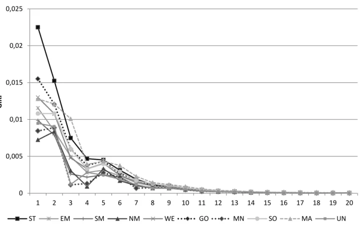
In Figure 4 we can see the generalized impulse response to the difference in house prices for each region corresponding to a one standard deviation shock in the change in
24 In this scenario, size would refer to population size and density, plus economic- and financial activity
towards the dominating region.
25
20 Stockholm house prices. The positive shock to the Stockholm market spreads throughout the remaining regions, raising the growth of prices in those regions over time. The shock appears to die out at around 12 quarters for all regions.
We can see that the initial shock to each region is larger than the shock to Stockholm after four quarters. We can also see that the effect of the shock is larger in the Malmo region after three periods compared to Stockholm; suggesting that the shock will be more durable over time for Malmo. This result indicates that the shock might die out slower over the spatial dimension compared to over time.
The results does not show any strong indications of the lead-lag effects; that the initial shock to Stockholm would take some time before affecting the other regions. The only three regions that appear to provide some lead-lag effects are the South, Middle Norrland and Northern Middle; as their responses do not peak at the direct contemporaneous shock but instead with a one period lag. The absent of lead-lag effects does not support the theories presented by Meen26 that a shock would spread in a ripple 26 See section 3. 0 0,005 0,01 0,015 0,02 0,025 1 2 3 4 5 6 7 8 9 10 11 12 13 14 15 16 17 18 19 20 G IR F
Figure 4 - Generalised impulse responses of a one unit shock (+ s.d.) to Stockholm on house price changes over time and across regions
21 pattern with some lag. This could however be logical in the sense that it is a difference between the theoretical ideas from a long-term increase in prices compared to a sudden exogenous shock, as in our case.
Figure 5 plots the responses in a figure with both space and time on the axes. The rate at which the shocks decays is captured by the decline going from left to right and the initial shock patterns for the spatial dimension is captured by the ridge going from right to left. The regions are ordered by their geographical distance from the dominant region; this is to see if geographical proximity to Stockholm plays a larger role for the contemporaneous effect.
The overall results from the impulse response analysis indicate that the most direct effect is on the Gothenburg, Malmo and Western regions. These results are not in line with the hypothesis that shocks to Stockholm would spread to neighboring regions in a
0 0,005 0,01 0,015 0,02 0,025
Regions orderd by distance from Stockholm Horizons in quarters
Figure 5 - Generalised impulse responses of a one unit shock (+ s.d.) to Stockholm on house price changes over time and across regions
22 higher degree than to regions geographically further away. Instead the shock to Stockholm seems to impact the other largest regions the most. This result can be seen as logical, as pointed out by Meen (1999), the spatial patterns of housing prices are subject to structural differences in the regional sub-markets and that these are important for explaining the spatial patterns. As Stockholm, Gothenburg and Malmo are the three major cities of Sweden, it is not unlikely that these markets are the most homogenous in terms of their structure.
Meen argues that these structural differences can rise from several factors, such as differences in behavior and housing stock. Also the similarities of type and rate of occupation, mortgage debt rates and access to other markets will be important factors in the heterogeneity between the sub-markets. Ferrari and Rae (2013) also argue that the British regional markets have become more heterogeneous over the past 40-years, and that migration is one of the most important factors for deciding the volatility of house prices. Their findings suggests that interregional migration is linked to socioeconomic factors and that migration is more likely to happen from a region with similar socioeconomic conditions. The linkage between the main cities of Sweden could be a result of migration between these regions due to the similarities they have in the context of socioeconomic conditions and occupational opportunities. Zhu et al. (2012) also find support for this argument as they find that in addition to migration flows, similar economic conditions in American regions also contribute to the spatial dependency of regional housing markets. Our findings are consistent with the findings of the above mentioned papers and indicate that spatial dependency should, perhaps, be modelled from a proximity measurement not contingent on geographical distance but instead proximity in the sense of economic and socioeconomic similarity.
7.
Conclusion
This paper uses the methodology of Holly et al. (2011) to try and estimate the spatial and temporal diffusion of house prices on regional Swedish data.
We find that Stockholm can be seen as a dominant region, as suggested by Chudik & Pesaran (2009) and that Stockholm is long-run forcing several of the other Swedish regions according to Granger & Lin (1995). We find that each of the regions responds
23 directly to shocks initiated in the Stockholm region and that some shocks are amplified by the neighboring regions in the following period.
Furthermore we find support that changes in GDP are significant in determining the house prices in the Stockholm region, acting in this context as a proxy for the general economic condition in Sweden.
Our impulse response analysis shed some light on the effect that shocks on Stockholm house market has on the remaining regions, where we can find certain evidence that the shock mainly affect the other two main cities of Sweden and that the shocks appear to dissipate faster over time than it does over space.
These findings are to some extent in line with previous findings in the area of spatial and temporal diffusion of regional house prices both in Sweden and in other countries. We do however find less evidence for the geographical proximity spillovers and the ripple effect, and instead find that other fundamentals in the regions might be of importance in modeling the spatial diffusion of house prices. Further research could be conducted into the modelling of the spatial matrix in order to better estimate the ripple effect of the regional housing market in Sweden.
24
8.
References
Abbott, A. and De Vita, G. (2013). Testing for long-run convergence across regional house prices in the UK: a pairwise approach. Applied Economics, 45(10), pp. 1227-1238.
Alexander, C. and Barrow, M. (1994). Seasonality and co-integration of regional house prices in the UK. Urban Studies, 31, pp. 1667-1689.
Barot, B. and Yang, Z. (2002). House prices and housing investment in Sweden and the United Kingdom. Review of Urban & Regional Development studies (RURDS), 14(2). Berg, L. (2002). Prices on the second-hand market for Swedish family houses: correlation, causation and determinants. International Journal of Housing Policy, 2(1), pp. 1-24.
Brady, R. (2014). The spatial diffusion of regional housing prices across U.S. states. Regional Science and Urban Economics, 46, pp. 150-166.
Can, A. (1990). The measurement of neighborhood dynamics in urban house prices. Economic Geography, 66, pp. 254-272.
Can, A. and Megbolugbe, I. (1997). Spatial dependence and house price index construction. Journal of Real Estate Finance and Economics, 14(2), pp. 203-222.
Chudik, A. and Pesaran, H. (2009). Infinte dimensional VARs and factor models. Working Paper Series, 998.
Clapp, J.M., Dolde, W. and Tirtiroglu, D. (1995). Imperfect information and investor inferences from housing price dynamics. Real Estate Economics, 23(3), pp. 239-269. Conley, T.G. (1999). GMM estimation with cross sectional dependence. Journal of Econometrics, 92, pp. 1-45.
Ferrari, E. and Rae, A. (2013). The spatiality of housing market volatility and selective migration. Town Planning Review, 84(1), pp. 107-125.
Giussani, B. and Hadjimatheou, G. (1991). Modeling regional house prices in the U.K. Journal of Financial Intermediation, 13, pp. 414-435.
Granger, C. (1969). Investigating causal relations by econometric models and cross-spectral methods. Econometrica. 37(3), pp. 424–438.
Granger, C. and Lin, J. (1995). Causality in the long run. Econometric Theory, 11(03), pp. 530.
25 Grossman, J.S. and Stiglitz, E.J. (1976). Information and competitive price systems. The American Economic Review. 66(2), pp. 246-253.
Gustafsson, P., Stockhammar, P. and Österholm, P. (2016). Macroeconomic effects of a decline in housing prices in Sweden. Journal of Policy Modeling, 38(2), pp. 242-255. Harter-Dreiman, M. (2004). Drawing inferences about housing supply elasticity from house price responses to income shocks. Journal of Urban Economics 55(2), pp. 316-337.
Helgers, R and Buyst, E. (2016). Spatial and temporal diffusion of housing prices in the presence of a linguistic border: evidence from Belgium. Spatial Economic Analysis, 11(1), pp. 92-122.
Himmelberg, C., Mayer, C. and Sinai, T. (2005). Assessing high house prices: bubbles, fundamentals, and misperceptions. Journal of Economic Perspectives 19(4), pp. 67-92. Holly, S., Pesaran, H. and Yamagata, T, (2010). A spatio-temporal model of house prices in the USA. Journal of Econometrics, 158(1), pp. 160–173.
Holly, S., Pesaran, H. and Yamagata, T. (2011). The spatial and temporal diffusion of house prices in the UK. Journal of Urban Economics, 69(1), pp. 2–23.
MaCarthy, J. and Peach, R. (2004). Are home prices the next bubble? Federal Reserve Bank of New York Economic Policy Review, 10(3), pp. 1-17.
MacDonald, R. and Taylor, M.P. (1993). Regional house price in Britain: long-run relationships and short-run dynamics. Scottish Journal of Political Economy 40(1), pp. 43–55.
Mahadeva, L. and Robinson, P. (2004). Unit root testing to help model building. Handbooks in Central Banking, 22.
McAvinchey, I.D. and Maclennan, D. (1982). A regional comparison of house price inflation rates in Britain, 1967-76. Urban Studies, 9(1), pp. 43-57.
Meen, G.P. (1990). The removal of mortgage market constraints and the implications for econometric modelling of UK house prices. Oxford Bulletin of Economics and Statistics, 52(1), pp. 1-24.
Meen, G.P. (1996). Spatial aggregation, spatial dependence and predictability in the UK housing market. Housing Studies 11(3), pp. 345–372.
26 Meen, G.P. (1999). Regional house prices and the ripple effect: a new interpretation. Housing Studies, 14(6), pp. 733-753.
Muellbauer, J. and Murphy, A. (1994). Explaining regional house price s in the UK. Working Paper WP94/21 (Dublin, University College Dublin, Department of Economics).
Munro, M. and Tu, Y. (1996b). The dynamics of UK national and regional house prices, Review of Urban & Regional Development Studies, 8(2), pp. 186-201.
Oikarinen, E. (2005) .The diffusion of housing price movements from centre to surrounding areas, ETLA Discussion Papers, The Research Institute of the Finnish Economy, No. 979.
Pesaran, M.H. and Shin, Y. (1998). Generalized impulse response analysis in linear multivariate models. Economics Letters, 58(1), pp. 17-29.
Pesaran, M.H., Schuermann, T. and Weiner, S. (2004). Modelling regional interdependencies using a global error-correcting macroeconometric model. Journal of Business and Economics Statistics, 22, pp. 129-162.
Stein, J.C. (1995). Prices and trading volume in the housing market: a model with down payment effects. Quarterly Journal of Economics, 110(2), pp. 379-405.
Tobler, W. R. (1970). A computer movie simulating urban growth in the Detroit region. Economic Geography, 46, pp. 234–40.
Wheelock, D. (2006). What happens to banks when house prices fall? U.S. regional housing busts of the 1980s and 1990s. Federal Reserve Bank of St. Louis Review, 88(5), pp. 413-429.
Yang, Z. and Turner, B (2016). Shock hunting: effects of dependent, regional-specific shocks in the Swedish property market. Housing, Theory and Society, 33(2), pp. 178-194.
Yang, Z., Wang, S. and Campbell, R. (2010). Monetary policy and regional price boom in Sweden. Journal of Policy Modeling, 32(6), pp. 865-879.
Zhu, B., Füss, R. and Rottke, N. (2012). Spatial linkages in returns and volatilities among U.S. regional housing markets. Real Estate Economics, 41(1), pp. 29-64.