Influence of Class Imbalance on Active Learning of Sleep EEG Classifier

(1)

Czech Technical University in Prague

Faculty of Electrical Engeneering

Department of Cybernetics

Influence of Class Imbalance

on Active Learning of Sleep EEG Classifier

Master Thesis

Supervisor: Ing. Martin Macaˇs, PhD.

Study programme: Biomedical Engineering and Informatics Specialisation: Biomedical Informatics

Bc. Nela Grimov´

a

(2)

Czech Technical University in Prague Faculty of Electrical Engineering

Department of Cybernetics

DIPLOMA THESIS ASSIGNMENT

Student: Bc. Nela G r i m o v á

Study programme: Biomedical Engineering and Informatics

Specialisation: Biomedical Informatics

Title of Diploma Thesis: Influence of Class Imbalance on Active Learning of Sleep EEG Classifier

Guidelines:

1. Make a survey, propose and implement criteria for evaluation of active learning. 2. Evaluate experimentaly active learning for data with different class imbalances. (Use synthetic data sets and observe the influence of class imbalance on performance of the active learning.)

3. Use the previous outputs for proposal, implementation and evaluation of active learning for detection of sleep stages from EEG signals (provided by the supervisor).

Bibliography/Sources:

[1] Settles, Burr. "Active learning literature survey." University of Wisconsin, Madison 52.55-66 (2010): 11.

[2] Ertekin, S., Huang, J., Bottou, L., & Giles, L. (2007, November). Learning on the border: active learning in imbalanced data classification. In Proceedings of the sixteenth ACM conference on Conference on information and knowledge management (pp. 127-136). ACM.

[3] Roederer, A. (2012). Active Learning for Classification of Medical Signals (Doctoral dissertation, University of Pennsylvania).

Diploma Thesis Supervisor: Ing. Martin Macaš, Ph.D.

Valid until: the end of the summer semester of academic year 2017/2018

L.S.

prof. Dr. Ing. Jan Kybic

Head of Department

prof. Ing. Pavel Ripka, CSc.

(3)

Declaration

I declare that the presented work was developed independently and that I have listed all sources of information used within it in accordance with the methodical instructions for observing the ethical principles in the preparation of university theses.

(4)

Acknowledgements

I would like to express my gratitude to my thesis supervisor Ing. Martin Macaˇs, PhD. for his guidance, valuable advice and willingness.

Furthermore, I would like to thank Ing. Václav Gerla, PhD. for being helpful in discussions about EEG data, Mgr. Kyriaki-Maria Saiti for her valuable comments and Mgr. Matˇej Bregant and Bc. Eliˇska Sekáˇcová for their corrections.

(5)

Abstrakt

Tato diplomová práce se zabývá aktivn´ım uˇcen´ım pro klasifikaci spánkových stav˚u na EEG datech. Jelikoˇz spánková data jsou obecnˇe nevyváˇzená, nejdˇr´ıve sledujeme, jak nevyváˇzenost na syntetických datech ovlivˇnuje aktivn´ı uˇcen´ı vyuˇz´ıvaj´ıc´ı strategii nejistoty a jej´ıch variant, které zohledˇnuj´ı rozm´ıstˇen´ı instanc´ı v prostoru. Je navrhnuto nˇekolik algoritm˚u, z nichˇz jeden uˇsetˇril v´ıce neˇz 80 % instanc´ı na ˇctyˇrech z pˇeti dataset˚u. Toto uˇsetˇren´ı je významné vzhledem k tomu, ˇze spánková data jsou anotována specialistou, který v souˇcasné dobˇe mus´ı ke vˇsem instanc´ım pˇriˇradit jejich tˇr´ıdu. V neposledn´ı ˇradˇe jsou v této práci navrhnuta vyhodnocovac´ı kritéria pro srovnán´ı metod aktivn´ıho uˇcen´ı ˇci pro zjiˇstˇen´ı, zda je navrˇzená metoda aktivn´ıho uˇcen´ı lepˇs´ı neˇz náhodný výbˇer instanc´ı.

Kl´ıˇcová slova: aktivn´ı uˇcen´ı; strategie nejistoty; EEG; spánkové EEG; vyhodnoc´ı

krit´eria

Abstract

This master thesis deals with active learning used for the classification of sleep stages on EEG data. Since sleep data are in general imbalanced, we first focus on how class imbalance of synthetic data influences active learning utilizing the uncertainty sampling strategy and its density-weighted variants. Several algorithms have been proposed, one of them saves more than 80 % of instances on four out of five datasets. These savings are significant with regard to the fact that sleep data are annotated by a specialist who must currently go through all instances and classify them. Last but not least, evaluation criteria are proposed in this thesis for the comparison of active learning methods or to verify if a suggested method is better than random sampling.

Keywords: active learning; uncertainty sampling strategy; EEG; sleep EEG; evaluation

(6)

(7)

List of Figures

1 Example of the three-class problem . . . 12 2 Initialization, four steps of the algorithm and the corresponding error,

first five steps of active learning are depicted in Figures 2a–2e, the corresponding error to these situations is shown in Figure 2f . . . 13 3 Initialization of active learning using the k-means algorithm, the class

ratio is 1:1 . . . 13 4 Initialization of active learning using the k-means algorithm, the ratio of

the first class to the second is 1:2 . . . 14 5 Initialization of active learning using the k-means algorithm, the class

ratio is 1:20. . . 15 6 Error on testing data of Banknote dataset and the percentage of unlabeled

instances whose class certainty is bigger than 75 % . . . 16 7 Mean error on classes on testing data of Banknote dataset of random

sampling and margin uncertainty sampling . . . 22 8 Synthetic Dataset 2 . . . 33 9 Miss rate of the minority class on the dataset with the class imbalance

ratio 1:20 and on the dataset with the class imbalance ratio 1:1 for random sampling and active learning . . . 36 10 Mean error on classes when undersampling methods with k = 2 and

k= 10 are adopted or when oversampling is used, MUS denotes margin uncertainty sampling . . . 37 11 Miss rate of individual classes when only margin uncertainty sampling

is used and when margin sampling together with oversampling is adopted 38 12 Mean error on class of margin uncertainty sampling strategy and three

density-weighted methods: DWD1, UMDN10 and UMDL. . . 38 13 Miss rate of individual classes when margin uncertainty sampling and

DWD1 strategy are used . . . 40 14 Miss rates of all classes on Sleep1 and Sleep2 datasets . . . 48 15 Miss rates of all classes on Sleep1 and Sleep2 datasets when observations

are classified into four (without NREM1 class) or into all five classes . . 49 16 Mean error on classes on Sleep1 dataset for different number of features

(10)

List of Tables

1 Visualization of the simplest confusion matrix . . . 17

2 Example of the confusion matrix . . . 17

3 The confusion matrix for a multiclass problem . . . 18

4 Error of three methods in each iteration . . . 23

5 Ranks of three methods in each iteration . . . 23

6 Percentage of values which are less than or equal to 0.15 in each iteration. Iterations after which 95 % of values are less than or equal to 0.15 are bold. . . 24

7 Summarization of determined criteria . . . 24

8 Description of datasets . . . 25

9 Evaluation criteria for Banknote dataset, threshold is set to 0.06. . . 25

10 Evaluation criteria for Pima dataset, threshold is set to 0.3. . . 26

11 Evaluation criteria for Spambase dataset, threshold is set to 0.27. . . 26

12 Evaluation criteria for Statlog dataset, threshold is set to 0.15. . . 26

13 Summarization of how many times active learning methods are better than random sampling in each criterion on all datasets. . . 27

14 Example of the confusion matrix of the imbalanced problem . . . 29

15 Mean miss rate of individual classes after 10, 100 and 1,000 iterations with different class imbalance of training data, strategy: margin uncertainty sampling. . . 34

16 Mean miss rates of individual classes after 10, 100 and 1,000 iterations with different class imbalance of training data, strategy: random sampling, dataset: 1. . . 34

17 Mean miss rates of individual classes after 10, 100 and 1,000 iterations with different class imbalance of training data, strategy: margin uncertainty sampling. . . 35

18 Mean miss rates of individual classes after 10, 100 and 1,000 iterations with different class imbalance of training data, strategy: random sampling. 35 19 Evaluation criteria for the second synthetic dataset with threshold set to 0.11. . . 39

20 Summarization of number of criteria in which the active learning method was better than random sampling . . . 39

21 Number of instances of each class for each dataset . . . 45

22 Evaluation criteria for Sleep1 dataset, threshold is set to 0.15. . . 45

27 Summarization of how many times active learning methods are better than random sampling in each criterion on all datasets. . . 47

28 Evaluation criteria for Sleep1 dataset when NREM1 class is excluded, threshold is set to 0.1 . . . 49

29 Evaluation criteria for Sleep2 dataset when NREM1 class is excluded , threshold is set to 0.1 . . . 50

(11)

1 Introduction

1.1 Motivation

In reality, when it comes to a lot of pattern classification problems of the real world, data instances are scarce and difficult to come by. Moreover, a situation is even worse when we are able to obtain some data but assigning them to a proper class is expensive or time-consuming. This includes applications, where a large amount of data is available but to divide them into categories is difficult (e.g. assigning of topics to documents [1]), or when a human annotator is needed.

The classification of sleep stages is a traditional task. A specialist studies a patient’s record of biophysical changes during the sleep (it is a record of EEG, EMG, EOM and ECG activity in most cases) and determines in which sleep stage the patient was. It is clear that this approach is tedious so there are tendencies to use machine learning techniques and automatize the process.

The main idea of active learning is to select a few of the most informative instances and use them in order to train a classifier. This process is based on asking queries about a class of the selected instance, and then the answer is provided by an oracle (e.g. by the specialist) [2]. Three strategies of how a query can be created will be discussed in Section 2.2.

It is assumed that as a result that a smaller amount of observations to learn a classifier will be needed and thus time and cost of assigning instances to their classes will be saved.

The aim of this thesis is to take the advantage of active learning methods and use them for classification of sleep stages, so the specialist will not have to annotate the whole record of sleep but only a few instances with the same achieved level of accuracy. Since stages of sleep are largely imbalanced, this fact hinders the traditional machine learning approaches, it is necessary to first figure out how a class imbalance influences active learning process.

1.2 Objectives

The first aim of this thesis is to conduct a survey about the current situation in active learning and also in addressing the class imbalance and as well to figure out which state-of-the-art methods are utilized.

Active learning methods are in most cases compared by the visual comparison of their values of a metric depending on the number of instances which were used for learning, so the other goal of the thesis is to propose criteria which can be utilized for an evaluation of active learning.

The next goal is to carry out experiments on synthetic datasets with different levels of class imbalance, evaluate them and observe how the class imbalance influences the performance of active learning.

(12)

The final step is to use the acquired knowledge for the application of active learning for detection of sleep stages in EEG signals, to implement chosen methods and to evaluate them.

1.3 Structure of the Thesis

We will provide the definition of active learning and mention all aspects connected to active learning in Section 2. Active learning is divided into three categories, according to which way the data used for learning are acquired. Then, we will mention strategies for selecting the most informative instances. We will especially deal with uncertainty sampling and density-weighted strategies, so these strategies will be discussed more in the last part of the second section, together with the initialization and the termination of active learning.

In Section 3, several metrics, which are used for evaluation of an algorithm performance, will be briefly introduced. Then it will be focused on evaluation of active learning, which is usually done visually. Several evaluation criteria that are suitable exactly for active learning will be proposed.

We deal with class imbalance in Section 4. The definition, what the class imbalance is, and what are the methods that are used for handling it, will be proposed. Then the connection between active learning and learning on skewed datasets will be described. We will perform experiments on synthetic datasets with different class imbalance and discuss them.

In Section 5, a brief introduction to sleep EEG will be provided and we will use results achieved in Section 4 for the utilization of active learning for detection of sleep stages. We will perform experiments on real data and discuss acquired results.

Results of the thesis will be summarized in the Chapter 6, they will be discussed and problems, on which it would be necessary to focus on in the future work, will be detected.

1.4 Types of Learning

Three categories of machine learning are often distinguished: supervised, unsupervised and reinforcement learning [3]. Let us provide a brief description of each category and also mention semi-supervised learning, which is a combination of supervised and unsupervised learning.

1.4.1 Supervised Learning

In supervised learning, we are given an instance (observation) spaceX, a state (class) spaceY and a probability densityPXY(x, y) which describes the joint probability that the instance xis observed and belongs to the class y. The goal of the task is to find a classifier f :X → Y which for every observation x ∈ X assigns its statey ∈ Y. It is expected that classifierf does not estimate the correct state yfor every observationx. Hence letL:X×X→R be a loss function which represents an amount of loss of the

(13)

estimated state due to the real state. Let yR be the real state and yE the estimated state, then L(yR, yE) returns the corresponding amount of loss.

When the number of classes is finite, we call this task classification [3]. Let us consider a typical classification task. We are given a set SSL of n pairs, each pair consists on the observation xi and its class yi: SSL = {(x1, y1), ...,(xn, yn)}, xi ∈ X,

yi ∈Y. We would like to find the classifierf such that its expected value of lossR(f) (also called a risk of the classifier [4]) is as small as possible:

f = arg min f:X→Y R(f) = arg min X x∈X X y∈Y L(x, f(x))PXY(x, y) (1)

With the zero-one loss function L01(y, f(x)), i.e. with the function which returns

0, if the estimated and the real state is equal, or 1, if the estimated and the real state differ, the risk becomes the classification errore:

e= X x∈X X y∈Y L01(x, f(x))PXY(x, y) (2) 1.4.2 Unsupervised Learning

Unlike in supervised learning, there is no knowledge about classes in unsupervised learning, only the observation spaceX is known. As an input, a program receives a set

SU L which containsninstances from X,SU L={x1, ..., xn}.

The goal of the task differs according to the application. It covers finding common features of data inSU Land cluster these instances intoksets (e.g. k-means clustering), the estimation of the probability densityPX or the dimensionality reduction [3].

1.4.3 Semi-supervised Learning

Semi-supervised learning is a combination of supervised and unsupervised learning. Let us assume an observation spaceX, a class spaceY and a probability densityPXY(x, y). Semi-supervised learning deals with both unassigned and assigned observations of the class.

Let SSSL be the input set of instances which is the union of sets SL and SU, i. e.

SSSL =SL∪SU. SLhas the same meaning as the setSSL in supervised learning, thus it is a set of m pairs of observations and their classes: SL = {(x1, y1), ...,(xm, ym)}. On the other hand, SU is similar to set SU L in unsupervised learning and contains

n instances from X without the assigned class: SU L ={xm+1, ..., xn+m}. Let us call instances from setSL labeled instances and instances from setSU unlabeled instances. Denote that it holds mn.

(14)

Labeled instances provide a prior knowledge about a problem and constrain the input space. A common example of semi-supervised learning is the semi-supervised variant of EM algorithm [5].

1.4.4 Reinforcement Learning

Reinforcement learning is often used in agent-based systems. Reinforcement learning is similar to supervised learning, but there is no prior knowledge about the setSSL. A set of agent’s actionsAand a set of statesT are given. An agent moves from the state

ti to the statetj,ti, tj ∈T by taking actions and exploring an environment. Each made action gives him a rewardr. Acquired knowledge helps the agent to higher ability of reasoning. [6].

1.4.5 Determination of Active Learning

Active learning can be considered as a part of semi-supervised learning (Section 1.4.3), although the term active learning also appears in literature about reinforcement learning [6], where it is used for the algorithm in which an agent actively searches through its environment. Note that active learning is also one of social psychology fields [7], but it has nothing in common with our topic.

(15)

2 Active Learning

A description of active learning will be given in this section. We will provide a brief motivation to answer the question why it should be given more attention in the field of active learning and what are its advantages.

2.1 Definition

Let X be the observation space and Y the finite state space. We are given a set of unlabeled instancesSUand a set of labeled instancesSL, which have the same meaning, as it is proposed in Section 1.4.3 and it holds that|SU|>>|SL|, the classifierf :X→Y and the oracleO for annotating selected instances.

The most informative observation x∗ ∈ SU is chosen in each step of an active learning algorithm according to the performance of the classifier f trained on labeled instances. The methods of creating queries will be discussed later. Let →O: X →

X×Y be the mapping which denotes that the oracle assigns a label to the observation. Selected instances are labeled by the oracle, i.e. x∗ →O (x∗, y), y ∈ Y, and (x∗, y) is added to the set SL.

It is required to answer several questions before implementing active learning. Firstly, as we have mentioned before, it can be difficult to obtain a set of unlabeled instancesSU. Processes of acquiring unlabeled instances will be described in the next section.

It is also needed to decide how the process will be initialized (i.e. how the initial set

SL will be created) and terminated. It will be mentioned in Section 2.4.3 and Section 2.4.4.

2.2 Unlabeled Instances Sampling

Sampling of unlabeled instances is divided in up to three categories: pool-based sampling, stream-based sampling and membership query synthesis [2,8]. Let us remark that pool-based and stream-based sampling can be also merged to one category called selective sampling, because of their similar features [1].

2.2.1 Pool-based Sampling

Regarding pool-based sampling many observations can be gathered at once. This amount of instances is called a pool and has the same meaning as the setSU which is defined in Section 1.4.3.

The main advantage of this approach is that we are allowed to compute a chosen informativeness measurement on all unlabeled instances and select the most informative one.

Instances are usually chosen sequentially, i.e. one instance is labeled at each iteration and the set of labeled instancesSLis used to retrain the classifierf. However, this process often appears to be expensive and inefficient in applications where training

(16)

the classifierfconsumes a great amount of time [9]. Therefore, active learning algorithms were invented in order to allow collecting more instances within one iteration. This approach is called batch-mode active learning [10].

Active learning using pool-based sampling was exploited in many applications, e.g. in the text classification [11], in the natural language processing [12] or in the artifacts detection of EEG signals [13].

2.2.2 Stream-based Sampling

Using pool-based sampling is often limited to cases when only a limited memory to store observations is available or when a data source, from which observations are gathered, is changing [2].

An algorithm samples an instance from its distribution PU and decides if the instance will be accepted as query or rejected. Stream-based sampling is often called sequential active learning because instances are gathered from data source one by one [2].

Stream-based sampling is also used when it is not necessary to keep a whole setSU and the easier and cheaper way is sampling observations right from their distribution. Note that the distributionPUdoes not need to be known but it is recommended that samples should come from non-uniform and real distributions [2]. If the distribution is uniform then stream-based sampling behaves like query synthesis which will be mentioned in the next section [8].

2.2.3 Query Synthesis

Only real instances are selected as queries in stream-based and pool-based sampling scenarios. Queries are generated by a learner in the query synthesis and are able to look like any instance from the observation space [14].

A learner can construct a query which is unrecognizable to human oracle, as it is often recommended to use query synthesis only for finite problems domains [2, 14]. Nevertheless, the efficient spectral algorithm has also been introduced, and it expands the possibilities to use query synthesis in more complicated settings as well [15].

2.3 Query Strategies

When active learning is adopted, one of the most important question to answer is how the most informative instances will be selected. A large number of them exist in literature [2], so the most common strategies will be mentioned in the following section. Note thatx∗_Arefers to the best query in accordance with the query strategy framework

(17)

2.3.1 Uncertainty Sampling

The uncertainty sampling is the most popular and the simplest strategy [2]. Uncertainty sampling was proposed by Lewis et al. [16]. It is suitable mostly for probabilistic models, but it might also be applied to non-probabilistic classifiers [2].

In this approach, the instance, whose label the classifier is least certain of, is queried. Three variants of uncertainty sampling are mentioned: margin uncertainty sampling, entropy sampling and the least confidence strategy [2].

Entropy sampling is often used because of its simplicity [17]. The instance with the biggest entropy is queried:

x∗_E = arg max x − |Y| X i=1 P_Y|X(yi|x) logPY|X(yi|x). (3) For problems with more than two classes, it is suitable to use least confidence strategy where the instance with the smallest posterior probability of the most probable label is sampled [18]: x∗_LC = arg min x (arg max y PY|X(y|x)). (4) This method takes into account only information about the most probable class, as a result margin uncertainty sampling was proposed by Scheffer et al. [19]. The idea behind this strategy is that the algorithm selects the instance with the smallest difference of the highest and the second highest posterior probability.

x∗_{M S} = arg min x

PY|X( ¯y1|x)−PY|X( ¯y2|x), (5)

where ¯y1is the most probable and ¯y2 the second most probable label of the instance

x.

2.3.2 Query by Committee

Query by committee framework have been introduced for the first time by Seung et al. [20]. A committee of c classifiers C = {θ1, . . . , θc}, which represents consistent hypotheses with labeled instances, are allowed to vote on the labellings of unlabeled observations. The instance, on which classifiers disagree the most, is considered as the most informative and is chosen as the query.

It is often supposed that embracing query by committee scenario results in a proper reduction of the version space [2]. The algorithm must to be able to create different hypotheses and compute some measure of disagreement among them. There have been several methods for measuring the disagreement proposed, e.g. the vote entropy [21] which is defined as following:

x∗_{V E}= arg max x |Y| X i=1 V(yi) |C| log V(yi) |C| , (6)

(18)

whereV(yi) is the number of votes that each labelyi receives.

Other methods include Kullback-Leibler divergence [1, 11] or F-complement, where F-measures between committee members are compared [1, 22].

2.3.3 Expected Model Change

The basic idea behind expected model change is that the learner should query the instance whose labeling would cause the greatest change of the current model.

Settles et al. [23] have introduced a strategy called expected gradient length. This approach is suited for learning using gradient-based methods. The instance, whose addition to the labeled set would cause the greatest change of the gradient, is queried. Expected gradient length approach has been applied to conditional random fields models (CRFs) [12], a similar strategy for CRFs has also been introduced by Vezhnevets et al. [24].

Another algorithm called expected model change maximization was proposed by Cai et al. [25], when it was used for linear and nonlinear regression.

2.3.4 Density-Weighted Strategy

The problems of using uncertainty sampling and query by committee frameworks cover a situation when the instance, about which the classifier is most uncertain (or with the biggest disagreement among committee members), is queried, but it does not sufficiently represent other instances [2]. As a result, Settles et al. [12] proposed the information density framework.

LetI(x) be the informativeness of the instancexgiven e.g. by uncertainty sampling or query by committee, s(xi, xj) be the function describing the similarity between xi andxj andβ ∈R be the weight of the similarity term. Then the algorithm queries an

instance for which it holds:

x∗_ID = arg max x I(x)× 1 |SU| |SU| X j=1 s(x, xj) !β (7)

2.3.5 Expected Error Reduction

This approach consists of computing error estimates of using SL ∪ (x, y), x ∈ SU on remaining unlabeled instances i.e. SU \ {x} and querying the instance x∗ whose addition to the setSL will result in the smallest future error [2].

Since true labels of unlabeled instances are not known, they are estimated by using the current classifier. The label of the instancex∗is also unknown, so its expected error is computed as the average over errors computed for all possible labeling weighted by the posterior probability given by the classifier [26].

(19)

2.3.6 Variance Reduction

Another approach of selecting the most informative instance consists of variance reduction of the expected error which can be easier and less expensive than reducing the expected error as a whole [2].

Settles et al. has introduced a selection strategy for sequence models based on Fisher information framework [18]. LetI_S_U(θ) be the Fisher information matrix of the set of unlabeled instances andIx(θ) be the Fisher information matrix of some instance

x, both above the model parameters θ. Then the most informative instance derives from:

x∗_{F I} = arg min x

tr(ISU(θ)Ix(θ)

−1₎_, ₍₈₎

where tr(A) denotes the trace of matrixA.

2.4 Algorithm

We will describe all the parts of active learning process in this section. Firstly, a description of a general version of active learning using pool-based sampling, which will be used further in this text, will be provided (see Section 2.4.1). Secondly, two new active learning strategies will be introduced (see Section 2.4.2).

2.4.1 General Version

The following pseudocode describes a general version of active learning which has a set of training data T R, the classifierf and variables, which depend on selected query strategy, as inputs.

Algorithm 1 Pool-based active learning

Input: set of training dataT R, classifierf, variables var

Output: set of labeled instances SL, trained classifierfT

[SA,SU] = initialize(T R)

SL = get label(SA)

repeat

fT = train classifier(SL,f)

x∗ = query strategy(SU,fT,var) (x∗, y) = get label(x∗)

SU =SU\ {x∗}

SL= SL∪(x∗, y)

f =fT

until terminal condition = true orSU =∅

The functioninitialize divides the set of training dataT Rinto the small setSAand the larger set of unlabeled instancesSU. Then the oracle is asked for labels of instances in the setSAby using the functionget label. Note that the input of this function can be

(20)

a single instance or a set of observations. Until the terminal condition is reached (this will be discussed more in Section 2.4.4), the algorithm loops: the classifierf is trained on the labeled set SL, then data from the set SU are classified, the most informative instance x∗ according to some query strategy is chosen, the function get label returns its labely andx∗ is removed from the setSU, while the pair (x∗,y) is added to the set

SL.

2.4.2 Strategies

Strategies that will be used in this thesis, will be described in this section. First of all, we will remind the margin uncertainty sampling strategy, we have already mentioned in Section 2.3.1, and the simplest version of the density-weighted strategy from Section 2.3.4. Furthermore, strategies called UMDN and UMDL will be proposed.

All strategies in the Algorithm 1 are called by the functionquery strategy.

Algorithm 2 Margin Uncertainty Sampling Strategy

Input: set of unlabeled dataSU, trained classifierfT

Output: instance x∗

min=∞

for allinstance x∈SU do

aposterior prob = get aposterior prob(x,fT)

subtract the biggest and the second biggest a posterior probability, save result into the variable c if c≤min then min=c x∗ =x end if end for

The most important part of this algorithm is calling the functionget aposterior prob

which returns the conditional probabilities of all classes givenx. The sum of those values is equal to one.

The simplest density-weighted method is very similar to uncertainty sampling, the certaintyc of an observation is multiplied by the mean distance to all other unlabeled instances. It is given by the value of β how much the certainty is affected by the distance. Let us denote this strategy as DWD*, where * is the value ofβ.

Density-weighted strategies called UMDN and UMDL will be introduced now. Let us describe UMDN strategy first (see Algorithm 3). Assume that we are able to get

l least certain instances by calling the function get l least certain. The least certain instances are obtained in the first part of the algorithm, then for each of these instances the nearest labeled observation is found. If the distance between them is larger than the maximal already received distance, the maximal distance is updated and the respective instance is queried. Similarly, as we have done before, let us denote this strategy as UMDN*, where * is the numberl, in order to distinguish these strategies with different parameters.

(21)

In UMDL strategy (see Algorithm 4),|Y|centroids of labeled instances are computed, with each centroid being the mean value of all labeled instances in the particular class. Certainty c and distanced from the nearest centroid are computed for each instance. Instance, whose product ofcand dis the smallest, is queried.

Algorithm 3 UMDN

Input: set of unlabeled data SU, set of labeled data SL, trained classifierfT, number

l

least certain= get l least certain(SU,fT,l)

max=−∞

for allinstance x∈least certaindo

d= get distance from the nearest neighbor(SL,x)

if d≥max then max=d x∗ =x end if end for Algorithm 4 UMDL

Input: set of unlabeled data SU, set of labeled data SL, trained classifierfT

centroids = get centroids(SL)

min=∞

for allinstance x∈SU do

aposterior prob= get aposterior prob(x,fT)

subtract the biggest and the second biggest a posterior probability, save result into the variablec

d= get min distance from centroid(x,centroids)

cd=c·d if cd≤minthen min=cd x∗ =x end if end for 2.4.3 Initialization

As we are aware of, the problem of how active learning process should be initialized, i.e. how to create the initial set of labeled instances, is not often followed up in the literature. Two different approaches exist: a random and an informative selection.

In the random selection, as the name suggests, instances to query are chosen arbitrarily. This approach is adopted e.g. from Ngai et al. [22].

Attenberg et al. [27] mentioned that researchers of active learning make one or two assumptions. First of them consists of presuming that the initial random selection

(22)

will provide a sufficiently accurate model to continue with active learning, the second reflects on the cold start problem – this means it is expected that the error of the classifier is high during several iterations at the beginning, whereas the set of labeled instances is small.

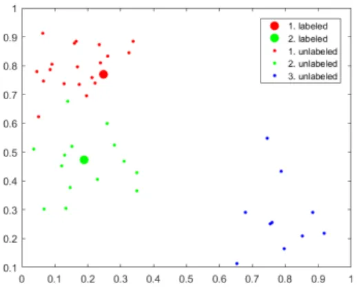
Let us demonstrate the cold start problem caused by the randomized initialization on the small example. Suppose two-dimensional data which we would like to classify into three classes. The margin uncertainty sampling strategy will be used (see Section 2.3.1) and a linear classifier [3]. The active learning process is initialized by the labeling of two randomly chosen instances. The initial situation is depicted in Figure 1.

Figure 1: Example of the three-class problem

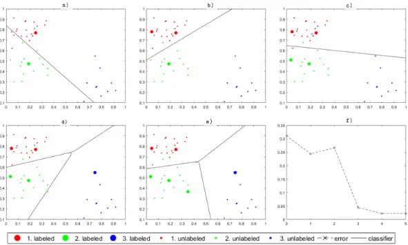
The labeled set SLcontains two instances belonging to two classes, while the third class is not represented. The initialization and first four steps of active learning are shown in Figures 2a–2e, the corresponding error on training data is depicted in Figure 2f.

The cold start problem covers the initial situation and another two steps of active learning (see Figures 2a–2c). As a result, the set of labeled instances SL does not contain any observation from the third class, as all data from this class are classified incorrectly, so the overall error is high. If the instance from the third class is added to

SL(Figure 2d), the performance of the classifier is improved. It is remarkable that this task is very simple and the third class was detected early after three iterations, but this problem can persist for a longer time in real world applications, when the task is more challenging or the environment is more complex.

Another technique for initialization is the informative selection of labeled instances. It involves a conscious choice of typical observations by a human annotator or some preprocessing step like e.g. the k-means clustering [3], where the observations closest to the acquired centroids are annotated [28], or the k-menoids algorithm which is based on the similar principle [29].

(23)

Figure 2: Initialization, four steps of the algorithm and the corresponding error, first five steps of active learning are depicted in Figures 2a–2e, the corresponding error to these situations is shown in Figure 2f

However, there are limitations of using this approach. Since this thesis deals with learning on imbalanced datasets, let us describe one of the problems caused by the informative selection on the following example. Suppose that in two-class problem, data are generated from two two-dimensional Gaussian distributions (µ1 = [0,2], σ1 =

[1,1.5; 1.5,3], µ2 = [2,3], σ2 = [1,1.5; 1.5,3]). Assume at first that number of instances

in both classes is equal, with data being depicted in Figure 3a. K-means algorithm withk = 2 was applied to these data and instances nearest to centroids were labeled. The result is shown in Figure 3b.

(a) Original dataset with class ratio 1:1 (b) K-means initialization with k= 2 Figure 3: Initialization of active learning using the k-means algorithm, the class ratio is 1:1

(24)

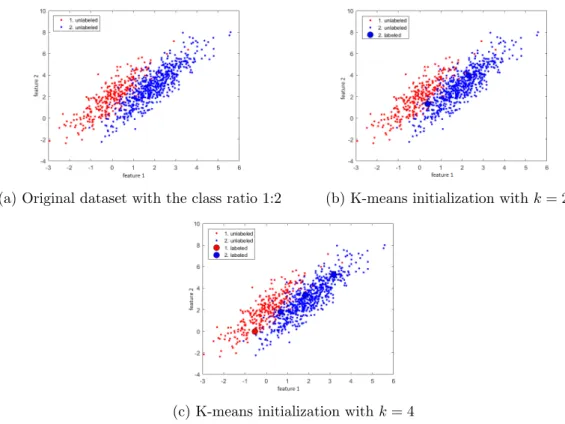
Now, suppose that there are twice less instances in the class 1 than in the second class. If we apply k-means with k= 2 as we did in the previous example, all selected instances would belong to the second class (see in Figure 4b). When we increase the number of centroids twice, k = 4, then the set of labeled observations contains data from both classes (Figure 4c). The original dataset is shown in Figure 4a.

(a) Original dataset with the class ratio 1:2 (b) K-means initialization withk= 2

(c) K-means initialization withk= 4

Figure 4: Initialization of active learning using the k-means algorithm, the ratio of the first class to the second is 1:2

We get similar results if we use the k-means algorithm on instances where the ratio of the first class to the second one is 1:20. Given labeled instances for differentk are shown in Figure 5. The original dataset is depicted in Figure 5a.

It is clear that with larger imbalance of classes it is necessary to search for more centroids to initialize active learning in the right way. We can expect that using some preclustering algorithm also causes the cold start problem in more difficult environments or when classes are very imbalanced.

Note the initialization, in which the set of labeled instancesSLcontainsnrandomly picked instances of each class will be used in our setting.

(25)

(a) Original dataset with class ratio 1:20 (b) K-means initialization withk= 2

(c) K-means initialization withk= 4 (d) K-means initialization with k= 6 Figure 5: Initialization of active learning using the k-means algorithm, the class ratio is 1:20.

2.4.4 Termination

Several conditions, which are used for termination of active learning, will be mentioned in this section. These conditions are:

• The number of iterations, which was determined in advance, is reached.

• Required value of a metric on testing data is reached. It is assumed that the chosen metric is computed in every iteration of the algorithm.

• Given percentage of unlabeled instances has bigger certainty value than some threshold. Note that this terminal condition can be used only if uncertainty sampling strategy or its variants are used.

• All instances in the margin are exhausted.

The metric, which we mention in the second bullet point, can be the given level of accuracy, error, F-measure, g-mean etc. These metrics will be discussed in Section 3.1. The terminal condition in the fourth option is also called the early-stopping criterion and it is used in active learning which exploits the SVM classifier for classification.

(26)

The main idea of this approach is that when all instances that lie along the margin are queried, the active learning process is terminated [30].

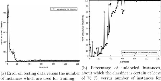
The third option will be discussed and shown on the example. Banknote dataset from UCI Machine Learning Repository [31] will be used. It is the two-classes dataset of 1,372 instances with four features, which was split into two sets of approximately the same size – training and testing set. The Parzen window estimator [32] is used as the classifier, margin uncertainty sampling is used as the query strategy and there are two instances of each class in the initial set of labeled instancedSL.

The error on testing data is depicted in Figure 6a. Assume that it is sufficient for us to be certain on the label of some instance at least on 75 %. We can see the percentage of unlabeled instances which certainty is bigger than this threshold in Figure 6b.

4 20 40 60 80 100 120 samples 0 0.1 0.2 0.3 0.4 0.5

mean error on classes

Mean error on classes

(a) Error on testing data versus the number of instances which are used for training

4 20 40 60 80 100 120 samples 0 10 20 30 40 50 60 70 80 90 100 % of unlabeled instances

Percentage of unlabeled instances

(b) Percentage of unlabeled instances, about which the classifier is certain at least of 75 %, versus number of instances for training

Figure 6: Error on testing data of Banknote dataset and the percentage of unlabeled instances whose class certainty is bigger than 75 %

The classifier is confident with at least 75% confidence about any label after forty-six iterations. There is a smaller decrease between fifty-five and fifty-eight iterations. Active learning would be stopped after forty-six iterations with the threshold of certainty set to 0.75 and threshold of percentage of instances set to 1. Note that algorithm would be stopped sooner if we set the mean error on classes to be at most 0.008 as the terminal condition. The process would be terminated after twenty iterations in that case.

(27)

3 Evaluation of Active Learning

The current situation of the active learning evaluation and the comparison of different active learning methods will be mentioned in this section. First, we will provide a introduction to several metrics that are commonly used for evaluation of standard machine learning methods.

3.1 Preliminaries

It is necessary to adopt some evaluation techniques to determine how correct is the trained model’s performance. Therefore, dataset is often divided into at least two parts – to training data, on which the classifier will learn, and to testing data. The partition of the dataset can be done at random, but it is highly recommended to use stratified 10-fold cross validation in real-world problems to reduce the influence of randomness [33].

3.1.1 Confusion Matrix

Several metrics for the classifier’s evaluation on testing data will be discussed in this section. All of them are based on the confusion matrix whose rows correspond to actual classes of the observation and columns to predicted states.

Consider the simplest case, i.e. the observation is either positive (belongs to the classy+) or negative (belongs to the classy−). If the observation’s actual and predicted

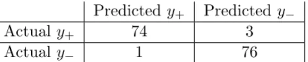
classes are both positive (or negative) then the observation is called true positive (negative, respectively). If an observation’s actual class is positive and its predicted class is negative, then it is notated as false positive, and contrariwise, if the actual class is negative and the predicted class is positive, then the observation is called false negative (see Table 1). The example, in which the classifier classified 150 instances correctly and four observations incorrectly, is shown in Table 2.

Table 1: Visualization of the simplest confusion matrix Predicted y+ Predicted y−

Actualy+ TP FN

Actualy− FP TN

Table 2: Example of the confusion matrix Predicted y+ Predicted y−

Actualy+ 74 3

Actualy− 1 76

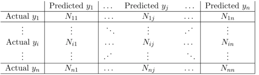
As we have mentioned before, this example is only the special case of the confusion matrix. In general, the confusion matrix is also defined for multiclass problems. Consider

(28)

a problem where observations are classified ton classes,Y =y1, . . . , yn. Let us denote

the number of observations whose actual class is y1 and predicted class isyn as N11,

the number of observations whose actual class is y1 and predicted class is y2 as N12,

etc. The corresponding confusion matrix is shown in the next table: Table 3: The confusion matrix for a multiclass problem

Predictedy1 . . . Predicted yj . . . Predicted yn Actualy1 N11 . . . N1j . . . N1n .. . ... . .. ... . .. ... Actualyi Ni1 . . . Nij . . . Nin .. . ... . .. ... . .. ... Actual yn Nn1 . . . Nnj . . . Nnn

It is possible for the specific classyi to convert the confusion matrix from Table 3 to the two-classes case. Let us defineT Pi,F Ni,F Pi and T Ni as follows:

T Pi =Nii (9) F Ni = n X j=1, i6=j Nij (10) F Pi = n X j=1, i6=j Nji (11) T Ni = n X j=1, i6=j n X k=1, i6=j Njk (12) 3.1.2 Metrics

Several metrics, which are used for the evaluation of classifiers, will be introduced in this section. Note that all described metrics take values from<0,1>, and they might also be expressed as percentage.

Let us remind the binary case as we proposed in Section 3.1.1 i.e. the goal of the task is to classify the observation as positive or negative, in order to adopt the confusion matrix (Table 1). There are several well-known metrics used for this binary case: the accuracyaccb, the precision precb, the sensitivitysensb, the specificity specb, the miss ratemissb and the fall-out f allb of the classifierf [34]. Let us define them as:

(29)

accb= T P +T N T P +T N+F P +F N (13) prec_b= T P T P +F P (14) sensb= T P T P +F N (15) spec_b= T N T N +F P (16) missb= F N F N +T P (17) f all_b= F P F P +T N (18)

values T P,T N,F P and F N are defined in Table 1.

The precision of the classifierf measures how precise is the assignment to the class

y+ [35]. It is defined as the proportion of correctly classified positive observations and

all positive classifications.

Since it is often inconvenient to manipulate with two metrics at the same time, several approaches, which combine two metrics into one, have been introduced. One of them is a geometric mean – g-mean which is in general defined as a square root of a two metrics’ product [36]. He et al. [35] provided two definitions of g-mean:

gm₁ =psensb×specb (19)

gm₂ =psensb×precb (20)

Other, the more sophisticated metric than g-mean, is the F-measure which is defined for any α∈R,α >0 as follows:

Fα= (1 +α2)

prec_b×recb (α2_×_prec

b) +recb

, (21)

where recb is the recall, another notion for the sensitivity. α is commonly set to one, then the F-measure is called F1-score [37].

We will generalize some of these metrics for a multi-class problem, i.e. a problem where|Y| ≥2.

The accuracy of classifier f is defined as:

acc= Pn i=1T Pi Pn i=1 Pn j=1Nij , (22)

(30)

corresponds to values in the confusion matrix given by the classifier f described in Section 3.1.1. The same goes forT Ni,F Pi and F Ni, discussed in metrics above.

Let us remind the error of the classifier e which was defined in Section 1.4.1. It holds that the accuracyaccis the complement of the e:

e= 1−acc (23)

The precision prec_i, the sensitivity sensi, the specificity speci, the miss rate (also called false negative rate)missi and the fall-out (also called false positive rate) f alli of the classifierf’s prediction of the class yi are defined as:

prec_i = T Pi T Pi+F Pi (24) sensi = T Pi T Pi+F Ni (25) spec_i = T Ni T Ni+F Pi (26) missi = F Ni F Ni+T Pi (27) f all_i = F Pi F Pi+T Ni (28)

It is noticeable that the miss rate is complement of sensitivity and also specificity and fall-out are complementary:

missi = 1−speci (29)

f all_i = 1−spec_i (30)

Let us define the mean precision on classesmprecand also the mean error on classes

meof the classifier as follows:

mprec= Pn i=1preci n (31) me= Pn i=1missi n (32)

It is also possible to compute F-measure for a multi-class problem. Micro-averaged and macro-averaged F-measures are often used. [38].

(31)

Let us define the micro-averaged F-measure M iFα as: M iFα = (1 +α2) p×r (α2_×_p_{) +}_r (33) p= Pn i=1T Pi Pn i=1(T Pi+F Pi) (34) r = Pn i=1T Pi Pn i=1(T Pi+F Ni) (35)

Macro-averaged F-measureM aFα is defined as:

M aFα= (1 +α2)Pn i=1 preci×reci (α2_×_prec i)+reci n (36)

Micro-averaged F-measure gives priority to the performance of a classifier to the larger of classes and macro-average F-measure to the minority class [38].

3.2 Active Learning Evaluation

In this section we will mention how active learning methods are compared and we will propose new criteria for evaluation of active learning.

3.2.1 Visual Comparison

As we mentioned before, active learning consists in the informative selection of one or more instance to query in each iteration of the algorithm. It is necessary to determine, if active learning will provide better results than if it had be done randomly. The most frequently used technique for evaluation, comparison to random sampling, or comparison of multiple active learning approaches is the visual comparison.

It typically consists of plotting a chosen metric as a function of the number of labeled instances, i.e. the number of instances which were used for training of the classifier. The metric is chosen according to the application, e.g. F-measure [1, 12], Area Under Received Operating Characteristic Curve [23, 27], accuracy [13, 28, 39] or the g-mean [40]. We will mostly use the error, the miss rate of individual classes and the mean error of classes.

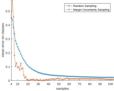
Due the fact that random sampling and also some active learning methods are stochastic, it is necessary to run the process several times in order to get more reliable results and use the average of the chosen metric through all runs of the algorithm for the comparison [23]. Let us show it on the example. We can see the comparison of active learning using the margin uncertainty strategy with random sampling launched on the

(32)

Banknote dataset in Figure 7, where is shown the mean error of classes depending on the number of labeled instances, results curve are achieved by averaging of 150 runs. We can see in Figure 7 that the active learning distinctly dominates over random sampling in all expect the first few iterations. It should be noted that it is not always straight-forward to make such clear conclusion about dominance of one algorithm.

4 10 20 30 40 50 60 70 80 90 100 samples 0 0.1 0.2 0.3 0.4 0.5

mean error on classes

Random Sampling Margin Uncertainty Sampling

Figure 7: Mean error on classes on testing data of Banknote dataset of random sampling and margin uncertainty sampling

3.2.2 Proposed Evaluation Criteria

Several criteria which can be embraced for evaluation of active learning and comparison of methods will be proposed. Let us denote that, as in the visual comparison part, it is necessary to compare an active learning method to random sampling in order to figure out if active learning leads to better results than a random sequential choice of instances.

Reaching Threshold

This criterion is the simplest one of all suggested criteria. It consists in defining the threshold (of the error, the mean error on classes, the accuracy, etc. on testing data) and determining how many iterations algorithm needs to reach this threshold. Then, all method are sort out in ascending order, the algorithm that has reached the threshold first is the best.

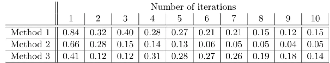
Let us show this criterion on example. Consider that if three methods are compared, the number of iterations is 10 and the corresponding error of all methods is shown in Table 4. Let us assume that the threshold is set at 0.15. Method 1 reaches this threshold after eight iterations, method 2 after three iterations and method 3 after two iterations.

(33)

Table 4: Error of three methods in each iteration Number of iterations 1 2 3 4 5 6 7 8 9 10 Method 1 0.84 0.32 0.40 0.28 0.27 0.21 0.21 0.15 0.12 0.15 Method 2 0.66 0.28 0.15 0.14 0.13 0.06 0.05 0.05 0.04 0.05 Method 3 0.41 0.12 0.12 0.31 0.28 0.27 0.26 0.19 0.18 0.14

This approach is straightforward, easy to implement and obviously reduces the number of labeled instances which are needed in order to train the classifier. The biggest disadvantage of this criterion lies in the choice of the threshold.

If active learning is compared to random sampling, we can interpret this criterion as the question: ”How many instances to training would we save if we exploited active learning?” The answer is the result of this criterion, when active learning is adopted and subtracted from the number of training instances.

Rank Comparison

Rank of all methods according to the chosen metric is computed in each iteration, i.e. if the mean error on classes is chosen as the metric, then the method with the smallest mean error on classes has the rank 1, the method with the second smallest mean error on classes has the rank 2, etc. The mean rank (computed over all iterations) of a method is computed for the overall comparison of all methods. Alternatively, the most frequent rank (mode) of the method can be used.

Let us remind the previous example and corresponding values of the error of the three methods in each iteration (see in Table 4). Matching ranks are shown in Table 5.

Table 5: Ranks of three methods in each iteration Number of iterations

1 2 3 4 5 6 7 8 9 10 Mean Mode

Method 1 3 3 3 2 2 2 2 2 2 3 3 2

Method 2 2 2 2 1 1 1 1 1 1 1 1.3 1

Method 3 1 1 1 3 3 3 3 3 3 2 2.1 3

Method 2 is the best of all methods according to both criteria, method 3 has the second best mean rank, however the most frequent value of its rank is 3, and the most frequent rank of the method 1 is 2, but the mean rank is 3.

The biggest advantage of this evaluation is that no external input is required as the threshold used in the previous evaluation technique and each method is directly compared to others. As we have shown in the abovementioned example, the mean of ranks and the mode of ranks produce different results so the decision which method is better rests with the user.

(34)

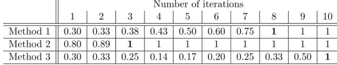
Breaking Point

The main idea of this evaluation criteria is in finding a point (iteration), after which a certain percentage of metric values would be bigger (e.g. if accuracy is adopted) or smaller (e.g. if error is computed) than the given threshold.

Let us consider the example again, the corresponding mean error of the three methods in each iteration is shown in Table 4 above. Let us assume that the point, after which 95 % of values of the error would be less than or equal 0.15 is being found. According to this criterion, method 2 is the best, as 95 % of error values are equal to 0.15 or smaller after three iterations. Method 1 reaches this point after eight iterations, method 3 achieves this after 10 iterations.

Table 6: Percentage of values which are less than or equal to 0.15 in each iteration. Iterations after which 95 % of values are less than or equal to 0.15 are bold.

Number of iterations 1 2 3 4 5 6 7 8 9 10 Method 1 0.30 0.33 0.38 0.43 0.50 0.60 0.75 1 1 1 Method 2 0.80 0.89 1 1 1 1 1 1 1 1 Method 3 0.30 0.33 0.25 0.14 0.17 0.20 0.25 0.33 0.50 1 Summarization

Let us summarize the results of our example in Table 7. The best results are marked in bold, the second best results are displayed in italics.

Table 7: Summarization of determined criteria

Reaching the threshold Mean Rank Mode of Ranks Breaking Point

Method 1 in 8 it. 3 2 in 8 it.

Method 2 in 3 it. 1.3 1 in 3 it.

Method 3 in 2 it. 2.1 3 in 10. it.

Method 2 reaches the best results, as it proves itself best in three out of four criteria. It is not easy to compare method 1 and 3, as method 1 is the second best in two out of four criteria, whereas method 3 is the best in the reaching the threshold criterion and the second best in the mean rank criterion.

3.3 Experiments

Several experiments on different datasets were conducted in order to evaluate some of the active learning strategies. We compare random sampling to these strategies: margin uncertainty sampling, the density-weighted strategy using the mean distance

(35)

to all instances as the similarity function with two different parameters and algorithms UMDN10 and UMDL from Section 2.4.2).

3.3.1 Data

Five datasets from UCI Machine Learning Repository [31] are used. We can see descriptions of the used datasets in Table 8, whereas the number of classes is stored in the column Classes, the number of features is in the column Features, the column Training instances denotes the number of instances, which are available to training, and the similar goes for the column Testing instances.

Table 8: Description of datasets

Dataset name Classes Features Training instances Testing instances

Banknote 2 4 684 684

Pima 2 8 384 384

Spambase 2 57 2281 2279

Statlog 7 19 1152 1151

3.3.2 Results

Selected stochastic algorithms (random sampling and margin uncertainty sampling) were launched 150 times. The number of iterations is 150. The mean error on classes was chosen as metric, the threshold for reaching the threshold and breaking point evaluation criteria was determined as the mean error on classes on testing data, when the classifier was trained on whole training data. The given percentage for breaking point criterion is set to 95 %.

All results are shown in the following tables, and one table corresponds to one dataset. The column RtT stands for the reaching the threshold criterion, MeanRC for the mean rank comparison, ModeRC for the mode of ranks comparison, BP for the breaking point comparison. The row RS stands for random sampling, MUS for margin uncertainty sampling, DWD1 for density-weighted method with distance function weighted by 1, DWD0.5 for density-weighted method with distance function weighted by 0.5. The best results are highlighted in bold and the second best in italics.

Table 9: Evaluation criteria for Banknote dataset, threshold is set to 0.06. Methods TRtT MeanRC ModeRC BP

RS 27 5.27 2 21 MUS 13 1.43 5 6 DMD1 13 2.38 3 7 DWD0.5 13 4.26 4 7 UMDN10 14 2.68 4 7 UMDL 13 4.97 1 6

(36)

Table 10: Evaluation criteria for Pima dataset, threshold is set to 0.3. Methods TRtT MeanRC ModeRC BP

RS 75 2.04 2 94 MUS 31 1.39 1 66 DMD1 116 4.38 5 115 DWD0.5 x 5.21 6 x UMDN10 72 3.36 3 146 UMDL 101 4.62 4 139

Table 11: Evaluation criteria for Spambase dataset, threshold is set to 0.27. Methods TRtT MeanRC ModeRC BP

RS 84 3.10 6 105 MUS 128 3.72 3 127 DMD1 35 2.15 1 29 DWD0.5 30 4.09 4 143 UMDN10 x 5.85 4 x UMDL 37 2.07 5 33

Table 12: Evaluation criteria for Statlog dataset, threshold is set to 0.15. Methods TRtT MeanRC ModeRC BP

RS 124 4.17 3 121 MUS 80 2.15 2 82 DMD1 103 3.39 4 102 DWD0.5 90 2.45 5 88 UMDN10 87 4.17 6 84 UMDL 122 4.67 3 122

The similar results on Banknote dataset are achieved by all active learning methods, margin uncertainty sampling is the best in three out of four criteria (TRtT, MeanRC and BP) and the same goes for UMDL algorithm (in criteria TRtT, ModeRC and BP). All active learning methods are better than random sampling expect of ModeRC criterion, where random sampling reaches the second best result.

Margin uncertainty sampling is a clear winner on Pima dataset, random sampling reaches the second best results in three out of four criteria, UMDLN10 strategy achieves the second best result in TRtT criterion. DWD0.5 strategy does not converge in 150 iterations, so it is overall at the sixth place.

DWD1 strategy is the best in two and the second best also in two criteria on Spambase dataset, DWD0.5 method reaches the best result in TRtT criterion and UMDL strategy in MeanRC criterion. Margin uncertainty sampling fails against random

(37)

sampling in three out of four criteria, UMDLN10 strategy does not converge in 150 iterations.

Margin uncertainty sampling reaches the best results in all criteria on Statlog dataset, UMDN10 is the second best in two criteria, UMDL and random sampling in one criterion.

It is very important to determine whether an active learning method is better than random sampling. The number we can see denotes when active learning methods reach better results than random sampling in Table13.

Table 13: Summarization of how many times active learning methods are better than random sampling in each criterion on all datasets.

Methods TRtT MeanRC ModeRC BP Sum

MUS 3 3 3 3 12

DMD1 3 3 1 3 10

DWD0.5 3 2 1 2 8

UMDN10 3 1 1 2 7

UMDL 3 2 2 2 9

Margin uncertainty is better than random sampling twelve times out of sixteen cases, DWD1 strategy ten times and UMDL strategy nine times. DWD0.5 is better only if the half of cases and UDMDN10 is better only seven times.

3.4 Discussion

We have proposed four evaluation criteria as an alternative to the most used method which is the visual comparison.

As we saw in Section 3.3.2, results of these evaluation criteria do not often match each other. It is difficult to determine which evaluation criterion provides the most reliable performance, so the more thorough analysis is needed. Despite this fact, we can recommend using these evaluation criteria in cases when it is not possible to evaluate which method is better according to the visual comparison.

Proposed criteria were used to identify in how many criteria some method reaches better results than random sampling. We used five methods on four different datasets, margin uncertainty sampling achieved the best results of all active learning methods compared to random sampling. It is still not possible to determine if margin uncertainty sampling is better than other proposed methods,as more datasets with the different number of instances, classes and features will be needed in order to do so.

(38)

(39)

4 Active Learning on Imbalanced Data

In this section we will provide the introduction to what imbalanced data are and what techniques are commonly used for handling the class imbalance.

4.1 Introduction to Class Imbalance

Machine learning can run into problems which are caused by the imbalance of classes. It often concerns real-world applications like biomedical, financial or security data analysis, text classification, face recognition, anomaly detection, etc. [35, 41, 42]

4.1.1 Characterization of Class Imbalance

The characterization of imbalanced datasets occurs when the number of instances in each class is not approximately equal, but some class (or classes) contains much more instances than other classes [41]. Class imbalance is often described by using the ratio of numbers of instances in the most common class to the rarest one. According to He et al. [35], if the ratio is 1:2, then datasets are marginally imbalanced, whereas they are modestly imbalanced with the ratio 1:10 and extremely imbalanced with the ratio 1:1,000.

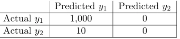
The problem of imbalanced data can be described in detail on the example. Consider a dataset which contains data belonging to two classes, e.g. the classy1 includes 1,000

instances and the class y2 10 instances. The corresponding confusion matrix is shown

in the following table.

Table 14: Example of the confusion matrix of the imbalanced problem

Predicted y1 Predicted y2

Actualy1 1,000 0

Actualy2 10 0

We will show the so-called accuracy paradox on this example [43]. Although this is a binary case, generalized metrics for a multi-class problem will be used because it does not hold that one class is positive and the other is negative. A standard classification method minimizing an errorf can classify all instances as classy1, so the accuracy of

the prediction accb is 99 %, but it is clear that the classifier does not solve the given problem. It seems to be more natural to use another metrics in this case.

As we mentioned in Section 3.1.2, the micro-averaged F-measure M iF gives the priority to the performance on the majority class and the macro-averaged F-measure

M aF on the minority class. Results correspond with this assumption, it holds that

(40)

As we mentioned before, as learning on skewed datasets is the common challenge, so a large amount of approaches to deal with it exists.

4.1.2 Sampling Methods

Sampling methods are used for creating the dataset with relatively balanced classes and two kinds of them exist: undersampling and oversampling [44].

In the case of undersampling, some instances of the majority class are removed. This process can be done randomly, which is easy for implementation but is also able to cause problems by removing informative instances, or there are techniques which removes only the redundant noise [35], e.g. modifications of the k-nearest neighbor algorithm [35, 45] or using of the soft margin SVM classifier [45].

Random oversampling consists of repeatedly copying of the minority class instances. Since this approach can lead to overfitting [35], Chawla et al. [46] have introduced SMOTE algorithm, which is able to create new synthetic instances. The main idea of SMOTE is the following: until the terminal condition is reached (generally as long as the classes are imbalanced), the randomly chosen instance from the minority class is chosen. Then, k nearest neighbors to the selected instance are computed and one is randomly chosen. Values of the new instance’s features are given by the difference between selected instances and its neighbor’s values of features multiplicated by the number between zero and one.

Hybrid techniques, which are the combination of SMOTE algorithm and an undersampling method, are also implemented [44].

4.1.3 Ensemble Methods

The main idea of ensemble methods is training of a group of classifiers and combining their decisions [47]. The crucial condition in using ensembles is that classifiers do not need to be accurate, but have to be diverse [42].

Several approaches are used for building ensembles, e.g. boosting algorithms such as Adaboost, Random Forest [35] or SMOTEboost (which is the combination of a boosting technique and SMOTE algorithm) [46].

4.1.4 Cost Sensitive Methods

In cost sensitive methods, the loss function is exploited which will largely penalize if the minority class instances are misclassified [35].

There are cost sensitive variants of favorite machine learning approaches e.g. a cost sensitive version of the SVM algorithm [35] or cost sensitive ensemble methods [41].

(41)

4.1.5 Insensitive Classifiers

Hoens et al. in [35] have mentioned the possibility of using classifiers which are in general skew-insensitive. One of them is naive Bayes because the conditional probability of the observationxi given the classy and the probability of the class y are computed before the conditional probability of the class y given the observationxi [35].

Decision trees are also skew-insensitive, e.g. Cieslak et al. [48] have proposed Hellinger distance decisions trees whose splitting criterion is Hellinger distance.

4.2 Class Imbalance and Active Learning

As we showed in Section 2.4.3, highly skewed datasets can cause problems during the initialization when it is impossible for the algorithm to find sufficient number of instances of all classes. Moreover, Attenberg et al. [35] have mentioned that active learning on extremely imbalanced data can suffer from the cold start problem because it is hard to find informative instances of the minority class due to their rareness.

In any case, opinions on active learning on imbalanced datasets differ. On the one hand, active learning can be used as the sampling method (see Section 4.1.2), on the other hand, it is often mentioned that active learning on skewed data can be problematic and there are approaches which enable active learning to learn a sufficiently accurate classifier [35]. We will explore both mentioned aspects in this section.

4.2.1 Active Learning as the Sampling Method

Attenberg et al. [35] and also Tomanek et al. [1] have mentioned that active learning can be effective on not extremely imbalanced datasets because it is able to choose the most informative instances.

The motivation for using active learning as the sampling strategy is that the final set of labeled instances SL is often more balanced than the initial pool [1]. It is supposed that it is more sufficient to use active learning to undersampling rather than some random selection of instances because random undersampling instead of active learning can discard the most informative observation.

Ertekin et al. [30] has proposed the VIRTUAL algorithm which combines active learning using SVM for classification and the SMOTE algorithm. The idea of the VIRTUAL algorithm is the following: When active learning selects the instance which comes from the minority class, then SMOTE is used, i.e. one of the k nearest neighbors of the selected observation is chosen and used for the creation of the new instance.

Zhu et al. [39] have suggested another active learning algorithm which combines both undersampling and oversampling. The set of labeled instances is resampled in each iteration of active learning; either the majority class is undersampled, or the minority class is oversampled by using the algorithm called BootOS, which iterates through all instances of the minority class and creates new instances as the combination of their neighbors.