Biomedical Data Classification with Improvised Deep Learning Architectures

ScholarWorks @ Georgia State University

ScholarWorks @ Georgia State University

Computer Science Dissertations Department of Computer Science

Summer 8-11-2020

Biomedical Data Classification with Improvised Deep Learning

Biomedical Data Classification with Improvised Deep Learning

Architectures

Architectures

Follow this and additional works at: https://scholarworks.gsu.edu/cs_diss

Recommended Citation Recommended Citation

Desai, Heta, "Biomedical Data Classification with Improvised Deep Learning Architectures." Dissertation, Georgia State University, 2020.

https://scholarworks.gsu.edu/cs_diss/161

This Dissertation is brought to you for free and open access by the Department of Computer Science at

ScholarWorks @ Georgia State University. It has been accepted for inclusion in Computer Science Dissertations by an authorized administrator of ScholarWorks @ Georgia State University. For more information, please contact

ARCHITECTURES

by

HETA DESAI

Under the Direction of Rajshekhar Sunderraman, PhD

ABSTRACT

With the rise of very powerful hardware and evolution of deep learning architectures, healthcare data analysis and its applications have been drastically transformed. These transformations mainly aim to aid a healthcare personnel with diagnosis and prognosis of a disease or abnormality at any given point of healthcare routine workflow. For instance, many of the cancer metastases detection depends on pathological tissue procedures and pathologist reviews. The reports of severity classification vary amongst different pathologist, which then leads to different treatment options for a patient. This labor-intensive work can lead to errors or mistreatments resulting in high cost of healthcare. With the help of machine learning and deep learning modules, some of these traditional diagnosis techniques can be improved and aid a doctor in decision making

and time in identifying the disease.

However, there are many other datapoints that are available with medical images, such as omics data, biomarker calculations, patient demographics and history. All these datapoints can enhance disease classification or prediction of progression with the help of machine learning/deep learning modules. However, it is very difficult to find a comprehensive dataset with all different modalities and features in healthcare setting due to privacy regulations. Hence in this thesis, we explore both medical imaging data with clinical datapoints as well as genomics datasets separately for classification tasks using combinational deep learning architectures. We use deep neural networks with 3D volumetric structural magnetic resonance images of Alzheimer Disease dataset for classification of disease. A separate study is implemented to understand classification based on clinical datapoints achieved by machine learning algorithms. For bioinformatics applications, sequence classification task is a crucial step for many metagenomics applications, however, requires a lot of preprocessing that requires sequence assembly or sequence alignment before making use of raw whole genome sequencing data, hence time consuming especially in bacterial taxonomy classification. There are only a few approaches for sequence classification tasks that mainly involve some convolutions and deep neural network. A novel method is developed using an intrinsic nature of recurrent neural networks for 16s rRNA sequence classification which can be adapted to utilize read sequences directly. For this classification task, the accuracy is improved using optimization techniques with a hybrid neural network.

ARCHITECTURES

by

HETA DESAI

A Dissertation Submitted in Partial Fulfillment of the Requirements for the Degree of Doctor of Philosophy

in the College of Arts and Sciences Georgia State University

Copyright by Heta Prakash Desai

ARCHITECTURES

by

HETA DESAI

Committee Chair: Rajshekhar Sunderraman

Committee: Michael Weeks Yanqing Zhang Yi Jiang

Electronic Version Approved:

Office of Graduate Studies College of Arts and Sciences Georgia State University August 2020

DEDICATION

To my loving, caring, kind and hard-working parents, who have sacrificed so much in life to provide me with opportunities to get a higher education and comforts of life. They are the epitome of loving and living life selflessly. My journey of becoming a scientist started long before I even started perusing my graduate studies. It started with my parents and older brother instilling me with curiosity towards nature’s wonders, perseverance for finding answers to scientific questions, and hard work to achieve those answers. Most importantly, their positive outlook to life has aided me in keeping my optimism high during the toughest times of my education journey.

To my second set of parents, my brother and sister-in-law who have always been my support system and have given me their unconditional love throughout my college education. My brother gave up on his masters to help me with my undergraduate funds. To my nephews, whose innocence makes my world so much brighter and motivates me to continue working in scientific research that would aid in making this world a better place for them and many future generations.

To my husband, who encouraged me and motivated me to work harder than ever before. He patiently listened to my countless ideas and random research talks, no matter how funny they seemed. He helped me think clearly to achieve my goals one at a time and continues to do so. His desire for my success is ten times higher than my own.

Finally, to my daughter, who was in my womb while I finished a lot of this dissertation work. She is constantly reminding me of how beautiful being a nurturer to the wonder of this nature is. The amalgamation of nature and machines that enhance research and lives have always fascinated me, hence my research interests have always been in interdisciplinary studies of physical sciences and engineering.

ACKNOWLEDGEMENTS

This work would not have been possible without many people. First and foremost, my kind-hearted advisor for guiding me since last 6 years; allowing me to work full-time during my first three years of graduate school and answering thousands of silly questions I have about computer science. Without his utmost support, encouragement and guidance, this work would not have been possible. We have had many thoughtful conversations regarding various research fields, and I am thankful for him for trying his best to provide me with resources needed to perform my research.

Secondly, to my committee members Dr. Michael Weeks, Dr. Yanqing Zhang and Dr. Yi Jiang. Dr. Weeks has taught me to be thorough, precise and punctual on my research as well as writing. Taking his class was one of the best ways I improved on my scientific writing. I took a few classes with Dr. Zhang, first was Computational Intelligence, in which I was introduced to some of the most crucial machine learning algorithms. He has been one of the humblest and understanding human being I have come across at Georgia State University. Lastly, Dr. Jiang whom I met at a talk she organized on “Chimpanzee and its behaviors” in Math department, which eventually became my masters’ project. I look up to her as a successful woman in science for her research and interest in multidisciplinary topics, which motivates me to be in multidisciplinary research.

Thirdly, I also want to thank my husband’s parents for understanding and helping at home while I drift away writing or doing my research. My extended family and friends who have always supported me when in doubt. I want to thank all my uncles, aunts, cousins and extended family who have been part of this tough journey. My friends, “the three musketeers” for always being

there for me, like always. I could not have possibly reached here without their support and long phone conversations.

Also, I want to thank all the administrative staff at the CS department, Ms. Rice, Ms. Pittman, Ms. Martin, Mr. Bryan and most importantly Ms. Dudley. Their presence truly makes the department more cheerful. Ms. Dudley has always maintained a smile and supported me through the tough times as well as always encouraged me to do better. She has been a friend, and a sister whenever needed to be. Thank you for everything you do for every student who knock on your doors every day. Lastly, I would like to thank all my colleagues at the department of Computer Science (CS), and Ms. Anuja P. Parameshwaran, who have become one of the closest friends within a short period of time. She has provided me with some of the core image processing techniques’ background during our brainstorming sessions.

I would like to acknowledge one of the quotes by a great scientist, engineer, artist and many other things, who have motivated me to explore many interdisciplinary areas. “Principles for the Development of a Complete Mind: Study the science of art. Study the art of science. Develop your senses- especially learn how to see. Realize that everything connects to everything else.” -Leonardo da Vinci

TABLE OF CONTENTS

ACKNOWLEDGEMENTS ... V

TABLE OF CONTENTS ... VII

LIST OF TABLES ... X

LIST OF FIGURES ... XI

LIST OF ABBREVIATIONS ... XIV

1 INTRODUCTION ... 1

1.1 Overview ... 1

1.2 Outline of contributions. ... 2

1.3 Medical image analysis ... 3

1.4 Dissertation outline ... 5

2 DEEP LEARNING ARCHITECTURES ... 7

2.1 Convolutional Neural Networks (CNNs) ... 7

2.1.1 A history of Convolutional Neural Networks ... 8

2.2 Recurrent Neural Networks (RNNs) ... 13

2.2.1 Simple Vanilla RNN... 13

2.2.2 LSTM and Bidirectional LSTM ... 14

3 REVIEW DEEP LEARNING APPLICATIONS IN MEDICAL IMAGING AND GENOMICS ... 16

3.1.1 Bacterial taxonomy classification ... 16

3.2 Brief Introduction to Medical Imaging Technology ... 23

3.3 Brief Introduction of Deep Learning applications in Medical Imaging ... 23

3.3.1 Localization/Detection ... 24

3.3.2 Classification ... 25

3.3.3 Segmentation ... 26

3.3.4 Registration ... 27

4 16S RIBOSOMAL GENE CLASSIFICATION USING RECURRENT NEURAL NETWORK AND CONVOLUTIONAL NEURAL NETWORK MODELS ... 29

4.1 Introduction ... 29

4.2 Dataset ... 31

4.3 Deep Learning Approaches ... 32

4.3.1 Simple vanilla RNN ... 34

4.3.2 LSTM and Bidirectional LSTM ... 35

4.3.3 Convolutional Neural Network and Multi-Filter CNN ... 36

4.3.4 Combinational Model ... 39

4.4 Results ... 39

4.5 Summary ... 43

5 DEEP ENSEMBLE MODELS FOR 16S RIBOSOMAL GENE CLASSIFICATION ... 45

5.1 Introduction ... 45

5.2 Method ... 49

5.3 Dataset ... 49

5.4 Deep Learning Approaches ... 50

5.5 Results ... 52

5.6 Future work for this study ... 56

6 ALZHEIMER DISEASE CLASSIFICATION USING DEEP LERNING ... 57

6.1 Introduction ... 57

6.2 Raw Dataset Preprocessing and Input Dataset Preprocessing ... 58

6.3 Multi-Data Deep Neural Network Model Architecture and Machine Learning Models 64 6.4 Results ... 67

6.4.1 Outcomes of Machine Learning Algorithms ... 67

6.5.2 Outcomes of Deep Neural Network ... 70

6.5 Summary ... 74

7 CONCLUSIONS AND FUTURE DIRECTIONS ... 75

LIST OF TABLES

Table 4.1 Final accuracies and losses of all six models for each family, genus and species

taxonomic levels. Accuracies highlighted in bold are the highest classification accuracy achieved within each level. *Stopped at 50 epochs since this model’s performance accuracy was dipping below 40%. ... 41 Table 5.1 Final accuracies and losses of all four models for each family, genus and species taxonomic levels. Accuracies highlighted in bold are the highest classification accuracy achieved

within each level. Precision, Sensitivity, F1 Score, Specificity, and Accuracy Data of Binary Classification Models... 55 Table 6.1 Subject demographics based on CDR score for number of MRI scans, MMSE score, Age at scan and entry, gray matter volume and education level scores. Except for MRI scan total, all other demographics averages were calculated alone with standard deviations. OASIS-3 dataset only provides with age at entry, hence firstly age at scan for each individual subject was calculated based on number of days between corresponding subsequence scans, following with averaged out age based on CDR scores. ... 68 Table 6.2 Precision, sensitivity, F1 score, specificity, and accuracy data of binary classification deep learning models using test data ... 72 Table 6.3 Precision, sensitivity, F1 score, specificity, and accuracy data of multiclass

classification deep learning models using test data ... 73

LIST OF FIGURES

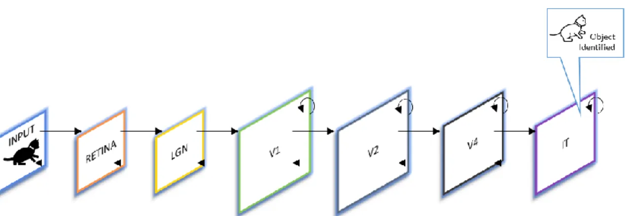
Figure 1.1 Overview of Artificial Intelligence and its popular classifiers ... 2 Figure 1.2 Overview of Health care Data type and Data Flow ... 4 Figure 2.1 Primary visual cortex and its functionality in image analysis. ... 7 Figure 2.2 The very first LeNet-5 architecture with 3 convolutional and 2 subsampling layers, with last one fully connected with classifier and output layer figure simplified to portray LeNet-5 from [21]. ... 9 Figure 2.3 Main architecture of AlexNet, with 5 convolutional layers and 3 fully connected layers with two separate Graphic Processing Units (GPUs), this is a simple illustration of

AlexNet. ... 10 Figure 2.4 This figure shows one of the inception modules introduced in GoogLeNet

architecture, which is shown stacked approximately nine time in overall architecture [11]. ... 11 Figure 3.1 Bacterial Taxonomy Classification, the focus of this study is on last three taxa,

Family, Genus and Species. ... 17 Figure 3.2 An example of localization task for brain lesions in Axial, hippocampus detection in sagittal and lesion in coronal sections ... 24 Figure 3.3 Classification is achieved by either detecting disease vs normal or by classifying the disease at different stages based on an input image normally a T1-MRI or FDG-PET scan. Above image is from OASIS-3 dataset example of four classes a) Cognitive normal, b) very mild

dementia c) mild cognitive dementia and d) Alzheimer’s disease. ... 25 Figure 3.4 Example of OASIS-3 dataset with ground truth of white matter segmentation. Bottom image shows the corresponding of above image for segmented white matter. ... 27

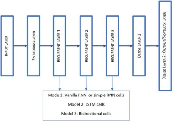
Figure 4.1: Overall architecture of data flow and RNN cell structures used in Model 1 (Vanilla RNN), Model 2 (LSTM) [29], and Model 3 (BiLSTM). ... 33 Figure 4.2: Illustration of the simplified model architecture where variable recurrent layer is dependent on RNN cell used. ... 35 Figure 4.3: A model architecture depicting A) Multi-filter (MF) CNN and B) simple CNN. Global MaxPool layer in B) serves as a flatten layer in this model. ... 38 Figure 4.4: A model architecture depicting combinational model. Global MaxPool layer serves as a flatten layer in this model. ... 39 Figure 4.5 The training and validation(testing) accuracies of A) family, B) genus and C) species level classification for all six models. ... 41 Figure 5.1: Overview of 16S rRNA sequencing application and motivation in bioinformatics... 47 Figure 5.2: Overall architecture of data flow of a) an ensemble model (depicted 3rd combination CNN-hybrid-LSTM), and b) hybrid model used for the classification task at hand. ... 52 Figure 5.3 The training and Validation(testing) accuracies of classification for family (a), genus (b) and species (c) level including both hybrid model and ensemble model. For ensemble model, accuracies shown here are from the best performing CNN-hybrid-LSTM model. ... 54 Figure 6.1 a) OASIS-3 dataset original subject distribution b) OASIS-3 number of PET and MRI sessions amongst male vs female distributions ... 59 Figure 6.2 Correlation of CDR vs Mini Mental State Exam (MMSE) and gray matter volume that shows a very high r-squared value of 0.9797 and 0.9907 respectively. A lot of other datapoints were measured for similar correlation, however, not all data had high correlation values. ... 60 Figure 6.3 Process flow of deep neural network models ... 61

Figure 6.4 An example of raw T1 MRI scan from OASIS-3 dataset without all of the pre-processing steps of intensity corrections, noise reduction, motion correction, skull stripping and normalization. Left most section shows axial plane, middle section shows sagittal plane and right most section shows coronal plane. ... 61 Figure 6.5 Raw data preprocessing: image extraction from MRI (.mgz) files and image storage folder structure ... 62 Figure 6.6 Input data preprocessing: splitting of training and validation data ... 63 Figure 6.7 An overview of multi-data convolutional neural network framework ... 64 Figure 6.8 Model architectures of individual plane slice for binary and multiclass classifications ... 65 Figure 6.9 Model architecture of multi-plane slices for binary and multiclass classifications ... 66 Figure 6.10 Population Distribution and Tess Accuracy data for binary classification using machine learning algorithm ... 69 Figure 6.11 Population distribution and test accuracy of various ML algorithms for multiclass classification ... 70 Figure 6.12 Training vs validation accuracy and loss graphs for each model ... 71 Figure 7.1 Combinational model to improve classification accuracies of Alzheimer’s disease for multi-class, multi-data input data ... 78

LIST OF ABBREVIATIONS

Georgia State University (GSU) Artificial Intelligence (AI)

Artificial Neural Network (ANN) Backpropagation through Time (BPTT) Computer-aided detection (CADe) Computer-aided diagnosis (CADx) Convolutional Neural Network (CNN) Deep Learning (DL)

Deoxyribonucleic Acid (DNA) Graphic Processing Units (GPUs) Rectified Linear Units (ReLU)

ImageNet Large Scale Visual Recognition Challenge (ISLVRC) Long Short-Term Memory (LSTM)

Machine Learning (ML)

National Institute of Health (NIH)

Medical Image Computing and Computer Assisted Intervention (MICCAI) Medical Imaging with Deep Learning (MIDL)

Magnetic Resonance Image (MRI)

Structural Magnetic Resonance Image (sMRI) Functional Magnetics Resonance Image (fMRI) Positron Emission Tomography (PET)

Open Access Series of Imaging Studies (OASIS-3) Recurrent Neural Network (RNNs)

Ribonucleic Acid (RNA) Ribosomal RNA (rRNA)

1 INTRODUCTION

1.1 Overview

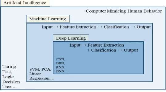
With the influx of large datasets and computational resources powerful enough to perform complex calculations, techniques of data analysis have also changed with broadened areas of applications [1]. With stronger graphic processing units (GPUs), scientists and researchers are now being able to collectively analyze data at a much larger scale than ever before [2], giving rise to the field of deep learning [3]. Today, deep learning has drastically changed the way images [4], videos, and textual data [5] have been studied collectively, quantitatively and qualitatively. More recently, the advancements in this field has also influenced applications in healthcare data analysis. In past before deep learning, it used to be very difficult to interpret, classify medical images or medical reports due to either limitations in publicly available dataset ; however, in last few years hundreds of papers have been published with advancement studies involving deep learning [6]; be automatic breast cancer detection [7], skin cancer lesion detection through a phone application [8] or diabetic retinopathy vessel segmentation [9]. The broad idea of artificial intelligence is that a computer can mimic a human behavior to aid in automizing a task. Figure 1.1 below illustrates an overall representation of artificial intelligence and its sub research fields of machine learning and deep learning.

Figure 1.1 Overview of Artificial Intelligence and its popular classifiers

1.2 Outline of contributions.

First focus of the study is to classify 16s rRNA bacterial gene based on its sequences. For this task below are the model architectures that are explored:

1) recurrent neural network (RNNs) are closely examined, especially Long Short-Term Memory (LSTM) dependent architectures.

2) Further, 1-dimentional convolutional neural networks (1D CNNs).

3) Combinational hybrid models consisting of both convolutional neural networks 4) Ensemble models involving hybrid models

This is one of the first study that investigates recurrent neural networks to classify 16S rRNA in their taxonomy. These pilot studies will help with future work in AI in healthcare implementing various deep learning architectures and by applying ensemble models of machine learning with deep learning.

Second focus of this study was to classify Alzheimer’s disease based on T1w MRI slices. For this study, an in-depth investigation is performed as below.

1) Eight convolutional neural networks for MRI medical images and two machine learning neural networks for clinical data are created.

2) Binary vs. Multiclass for all 10 models classification explored 3) Regression analysis to find highly correlated clinical data

4) A concatenated model architecture to utilize all slices from three planes, axial, sagittal and coronal.

1.3 Medical image analysis

There are mainly two type of applications of artificial intelligence in medical image analysis: 1) Computer-aided detection (CADe), 2) Computer-aided diagnosis (CADx). CADe is to identify an abnormality in region of interest and to improve detection rate of such regions with lowering the false negative rate. Typically, in CADe, the region of interest is detected with image processing techniques, features are represented as statistical information and features are fit. CADx are known for its discrimination of malign or benign lesions. There are both unsupervised and supervised learning methodologies used in networks with majority being supervised learning. With the rise of personalized medicine and electronic health records, National Institute of Health (NIH) is also bringing some standards with such technologies in order to be deployed and used in real time, including standards in radiology reports of such imaging [10, 11].

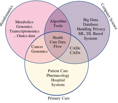
Figure 1.2 Overview of Health care Data type and Data Flow

Regardless of many successful studies of deep learning in medical image analysis, the biggest challenge right now is analyzing different sources of data collectively. One of the main ideas of this study is being able to collectively analyze and utilize all patient data that is available for AI in healthcare to aid in an end-to-end pipeline in future. Healthcare data today has three main sources, 1) any omics data such as genomics, proteomics, metagenomics, or transcriptomics etc. related to patient and/or diseases, 2) medical images from various modalities for disease detection/progression/classification/segmentation, and 3) textual data such as doctor’s notes, chief complains, symptoms, pathology/radiology reports, hospital care details, etc. These three datatypes belong to three separate areas of research, 1) bioinformatics, 2) computer vision and 3) natural language processing respectively. Each research area is vast, but have to be studied in order to understand overall complexity of data analysis. Most of the models are either modality

Primary Care Metabolics Genomics Transcriptonomics ...Omics data Big Data Database Handling Privacy ML, DL Based Systems Patient Care Pharmacology Hospital Systems Cancer Genomics Health Care Data Flow Algorithm Tools CADe CADx

dependent or organ/disease dependent for the image processing tasks to work effectively. In order to help through an automatic detection, this study attempts to suggest some deep learning systems can come together and serve as a template.

1.4 Dissertation outline

This dissertation is organized in total of seven chapters including Chapter 1. In this dissertation we solved two classification problems from two different areas of 1) bioinformatics and 2) medical image processing by developing several neural network architectures and overcoming some of the challenges pertaining to tasks. We provide a foundation for understanding neural network architectures and problems at hand in Chapters 2 and 3. In Chapter 4, 5 and 6, we provide the contributions made in this dissertation. Lastly, in Chapter 7, we provide a brief reflection on this research work and future directions.

Chapter 2, we offer an overview of deep architectures, CNNs in chronological order of

their more recent development utilized in medical image classification, and RNNs with explanation of basic architectures utilized in later chapters of genomics sequence classification.

Chapter 3, we provide background information necessary to lay foundation for understanding

medical image classification and genomics sequence classification tasks. In this chapter we also provide related works of both aforementioned classifications along with background information on application of deep learning in different areas of medical images and genomics.

In Chapter 4, we tackle the problem of deoxyribonucleic acid (DNA) sequence

classification. That is, provided a sequence of bacterial 16S rDNA sequences, predict the corresponding taxonomy at family, genus and species levels. We approach this problem as a textual classification problem with fixed length input lengths of input sequences. In this initial chapter, we used basic recurrent neural networks and convolutional neural networks to for

classification bacterial sequences into taxonomical representation. The content of this chapter is based on initial model architectures from Desai et.al [12] and comparison study of initial architectures with convolutional neural networks from Desai et. al [13]. Chapter 5 is an extension

of chapter 4, where we compare ensemble and hybrid models of recurrent neural networks and convolutional neural networks to see if an ensemble models without any further modifications in data can achieve state-of-the art performances. This chapter is based on methodology section of Desai et. al [14]. Chapter 6 is multi-data study performed on brain MRI dataset to classify Alzheimer’s disease for imbalanced dataset which is normally seen in real world applications especially in healthcare and biology. In this chapter we create a model architecture to separately observe clinical data information based on heavily utilized machine learning algorithms, as well as deep learning architectures that utilizes all three planes of a structural magnetic resonance imaging (sMRI). We also anticipate a major improvement on model architecture that combines both approaches to bring both model in same multimodal feature space. Finally, Chapter 7

concludes this dissertation with challenges and some of the ways to avoid bias in such deep architecture dependent technologies in healthcare. We also lay a path forward for some of the improvements to solve existing challenges.

2 DEEP LEARNING ARCHITECTURES

2.1 Convolutional Neural Networks (CNNs)

From the moment we wake up in the morning and open our eyes, our brain starts processing visual information around us. Unconsciously, all the information is compartmentalized and identified by just looking at a scenery. One looks outside a window and can identify tree, sunshine, clouds, birds, buildings etc. We also identify minute things, make correlational examination and make assumptive decisions from what we see. All these things are going on in our brains every day, intuitively we link objects with what they are linguistically called and make an instant label. These are all very complex processing, but we grow up learning things by labeling and making connections of objects to language. For instance, a child is shown a picture of a bird and is taught the spelling as well as verbal pronunciation of the word. These object identification task has been taught to us by repetitive example correlational research from an early age. Such model is an inspiration to machine learning paradigm or training and testing data to find correlation and patterns. Eye is the first contact point of this visual system; however, processing happens in area of the posterior part of brain called as primary visual cortex as seen in figure 2.1 below [15].

The inspiration behind CNN can be better understood by observing animal’s visual cortex. In 1960s, two researchers from Harvard Medical School, Dr. Hubel and Dr. Wiesel, first published a model on mammalian visual system (studies done of cats) showing how cells in primary visual cortex perceives surrounding world visually. Eyes see a small sub-regional scene, called receptive (visual) fields, normally divided in left visual field and right visual field. Visual cortex of brain receives these visual fields as an input. These small inputs are normally put together in series of slides to cover the entire receptive field. In visual cortex, there are two type of biological cells that play a very crucial role in the way our brain processes an image. These two cells are known as simple cells (S cells), and complex cells (C cells) [16, 17]. The simple cells are activated during edge detection, pattern tasks at a fixed angle view while complex cells are activated during larger receptive field without any restrictions on the view angle or position. This cascading model of S cells and C cells works together in pattern recognition. The receptive field in retina receives a stimulus that activates neurons in that field, which in return sends a somatic signal to downstream neuron bodies. Such information is passed in hierarchy and is stored in the order it is received, in terms sequential. The part of the brain that is involved in memories called neocortex, stored such information hierarchically.

2.1.1 A history of Convolutional Neural Networks

Recently, CNNs architecture have been making headlines with its various applications in robotics, disease/cancer classification, self-driving cars etc. However, the history of CNNs rather started in late 1980s Fukushima first proposed a neural network called neocognitron, a network with “an ability of unsupervised learning, learning without a teacher” [18]. This model was indeed inspired by previously mentioned “S cell/C cell” model proposed by Dr. Hubel and Dr. Wiesel, where an architecture was made with Simple cells, where parameters were modified with a layer

of complex cells, where pooling is performed [18, 19]. Much later in 1998, a group of researchers, Le Cun, Bottou, Bengio and Haffner, published a “Gradient-based learning” applied for document recognition. This study revealed the first ever Convolutional Neural Network, which they called LeNet-5.

Figure 2.2 The very first LeNet-5 architecture with 3 convolutional and 2 subsampling layers, with last one fully connected with classifier and output layer figure simplified to portray LeNet-5 from [20].

They proposed many versions of CNNs in their paper, with LeNet-5 being the best architecture, which was used to identify digits from hand-written numbers [20]. LeNet-5 as shown in the figure 2.2 above, have three main layers, convolutions, subsampling (pooling) and non-linearity (with tanh or sigmoid). This basic components of CNNs is used in image classification tasks in deep learning till date. Each layer of CNNs is explained in later sections in detail.

After a decade long gap, with the rise of graphical processing units (GPUs); automatic image classification, object detection, and speech recognition tasks came about in lime-light as well as rise of large image datasets. In 2009, a very well-known computer science professor Fei-Fei Li

opened an ImageNet Large Scale Visual Recognition Challenge (ISLVRC), consisting of labeled image dataset available to researchers, professors and students. In 2010, Ciresan and Schmidhuber came up with the first implementations of neural networks using NVDIA GTX 280 GPU with up to nine-layer neural network. Shortly after that, in 2012, Alex Krizhevsky, Sutskever and Hinton, proposed a much deeper architecture than LeNet and called it AlexNet in the ImageNet competition [21]. The architecture won the competition with 16.4 % error rate on classification task using AlexNet [22].

Figure 2.3 Main architecture of AlexNet, with 5 convolutional layers and 3 fully connected layers with two separate Graphic Processing Units (GPUs), this is a simple illustration of AlexNet.

One of the major contributions in architecture was of using rectified linear units (ReLU) as non-linearity functions after the convolutional layer instead of tanh or sigmoid, used data

augmentation techniques on input data, dropout layer to reduce overfitting on training data, and overlapping max-pooling. In 2013, the winner of ImageNet competition was ZFNet, found by Zeiler and Fergus. The architecture was very similar to AlexNet with some modifications involving filter size changes, introduced cross-entropy loss for error function and training using batch stochastic gradient descent. The model’s final error rate was 11.2% almost 5% less than AlexNet, by mainly fine-tuning the existing model. The researchers also developed a visualization technique called Deconvolutional Networks (DeConvNet) for different feature activation at each layer. In 2014, two architectures became popular, one GoogLeNet (the winner of the competition) and the other VGG [23]. GoogLeNet was a 22-layer CNN achieved 6.7 % of error rate. This was one of the first CNN architectures that created a very different architecture and deviated from stacking of the core of three-layer CNN architecture, Convolution-pooling-nonlinearity together. The main contribution of this paper was to introduce an inception module, which consists of different filter combinations of small convolutions 1 x 1, 3 x 3 and 5 x 5. These convolutions are concatenated at the end each inception module to pass to the next layer hierarchically. Figure 2.4 below shows one of the inception modules from GoogLeNet.

Figure 2.4 This figure shows one of the inception modules introduced in GoogLeNet architecture, which is shown stacked approximately nine time in overall architecture [11].

In this architecture, several inception layers are stacked together to create the final architecture. Another popular architecture, a runner-up from 2014 ILSVRC competition was VGGNET, developed by the Visual Geometry Group (VGG), University of Oxford. This network contributed in identifying network’s depth as one of the potential hyperparameter to achieve better recognition. The networked used two convolutional layers followed by an activation layer of ReLU; however, used three fully connected layers at the end in all proposed architectures [22]. Six variants of VGGNET were proposed the same year, VGG A through E; although, three of these six are now widely known as VGG-E (A), VGG-16(C) and VGG-19(E) [24]. All of them had similar architecture, except varying numbers of two convolutional layer + ReLU units; with VGG-E having total of eight convolutional layers, VGG-16, thirteen and VGG-19, sixteen such layers [24].

In 2015, another popular CNN architecture – Residual Network (ResNet) won the competition ILSVRC, proposed by Kaiming He from Microsoft Research Asia. It brought error rate down to 3.57%, much lower than the human error rate of 5 % [22, 25]. ResNet was proposed with many varying numbers of convolutional layers: 34, 50, 101, and 152.

This architecture deviated from the rest vastly as it introduced “a residual block”. This block goes through the series of convolutional layer – ReLU – convolutional layer, gives you some output, let’s say F(x). Now this output is added to the input x, so finally you get F(x) + x, whereas, in popular CNN, the output would be only F(x).

After the release of such powerful architectures, a lot more variants came out most recently. CNNs architectures performs the best, when the input data has a very structural component, such as an image or an audio with repeating patterns [26].

2.2 Recurrent Neural Networks (RNNs)

2.2.1 Simple Vanilla RNN

Recurrent neural networks (RNNs) are known to be temporally deep networks i.e. the RNNs are usually unrolled or unfolded in time. There are certain formulas that govern the computations of the RNN and they are: 1) input xt which is associated at time step t. 2) hidden state ht, or in other

words the memory which is calculated by taking the previous hidden state (at the previous time step (t-1)) and present input into consideration. i.e. ht = f (Uxt + Wht-1), where U, W are shared

parameters associated with the different layers of RNN and f is a nonlinearity functions which is generally a tanh function or a ReLU function. 3) output ot at time step t.

The vanilla RNN cell unit is a simple unit where the previous hidden state ht-1 and current

input xt is passed through the tanh non-linearity function to update the current hidden state, i.e.

equation 2.1 as below.

ℎ_𝑡 = 𝑡𝑎𝑛ℎ 𝑊(_ℎ

𝑡−1

𝑥𝑡 ₎

Equation 2.1

The drawback of vanilla RNNs is that it is difficult to train these networks. The updating of parameters for Vanilla recurrent neural networks happen the same way as that of artificial neural networks i.e. through the back-propagation algorithm. The catch with respect to the calculation of gradients at every time step is with respect to that fact that vanilla RNNs have shared parameters between all-time steps of a layer, as opposed to independent parameters of an ANN. Thus, to calculate a gradient in a current time step there is a need to backpropagate to previous time steps until the present one making the vanilla RNN have difficulties in learning long term dependencies i.e. dependencies between far away time steps. This backpropagation algorithm is called Backpropagation through Time (BPTT) and this can lead to the vanishing/exploding gradient problem. [27] Better variants of the RNNs like the LSTMs and the GRUs have been designed to

solve this problem, thus making these variants popular for tasks like sequence classification and prediction.

2.2.2 LSTM and Bidirectional LSTM

More variants of RNNs were developed to address the shortcomings of a simple vanilla RNN. LSTMs are a popular variant of RNNs, each unit of the LSTM is associated with memory typically called as a cell. In a LSTM cell unit, the memory is regulated with the help of three gates namely input gate (𝑖𝑡), output gate (𝑜𝑡, hidden state ℎ𝑡) and forget gate (𝑓𝑡), which helps determine which information needs to be added to the current cell state (𝐶𝑡) and which information can be forgotten to update the cell state. The equations 2.2 to equation 2.7 below represents the data flow from the current cell state, previous cell state and the next state. [28]

𝑓_𝑡 = 𝜎(𝑊_𝑓∙ [ℎ_𝑡−1, 𝑥_𝑡] + 𝑏𝑓) Equation 2.2 𝑖𝑡= 𝜎(𝑊𝑖 ∙ [ℎ𝑡−1, 𝑥𝑡] + 𝑏𝑖) Equation 2.3 𝐶̃𝑡= 𝑡𝑎𝑛ℎ(𝑊𝐶∙ [ℎ𝑡−1, 𝑥𝑡] + 𝑏𝐶) Equation 2.4 𝐶𝑡= 𝑓𝑡∗ 𝐶𝑡−1+ 𝑖𝑡∗ 𝐶̃𝑡 Equation 2.5 𝑜𝑡 = 𝜎(𝑊𝑜∙ [ℎ𝑡−1, 𝑥𝑡] + 𝑏𝑜) Equation 2.6 ℎ_𝑡 = 𝑜_𝑡∗ 𝑡𝑎𝑛ℎ (𝐶_𝑡) Equation 2.7

The advantages of the LSTMs over vanilla RNNs are that they were specifically designed to overcome the vanishing gradient problems and are deemed efficient in capturing long-term dependencies. Due to the vanishing gradient problem in Vanilla RNN models, LSTM were introduced since its ability to update its own cell-state. In LSTM unit, the horizontal line on top acts as a “conveyer belt – with some minor linear interactions,” making backpropagation task much simpler [28].

Bidirectional LSTMS capture the idea that the output of recurrent unit at a time step not only depends on its past instances (past elements of the sequence) but also on the future instances. The idea of such a network is developed by stacking 2 layers of LSTMs over each other thus

making the output dependent on the computation of hidden states from both the LSTM layers as opposed to one as in the unidirectional LSTM network.

3 REVIEW DEEP LEARNING APPLICATIONS IN MEDICAL IMAGING AND

GENOMICS

3.1 Relevant Deep Learning applications for biomedical data in Literature

With impressive breakthroughs in computer vision and natural language processing, and due to its power of being able to identify intrinsic features within the dataset, deep learning has drawn attention of almost every interdisciplinary researcher even out of computer science domain. This chapter focuses on background of two main applications of deep learning in, 1) sequence classification in genomics and 2) disease diagnosis/classification with medical imaging data. Within genomics, this dissertation focuses on bacterial taxonomy classification, and within medical imaging, this dissertation focuses on Alzheimer’s disease classification using structural MRI. For each section, dataset, methods, architectures and results are discussed in detail.

3.1.1 Bacterial taxonomy classification

There have been many machine learning approaches in solving genomics problems, more recently, deep learning approaches are also appearing with tools to solve many popular problems related to human genomes, especially in functional and regulatory genomics. In functional genomics, prediction of DNA sequence specificity to RNA binding protein cis regulatory cites, gene expression, methylation status and chromatin immunoprecipitation (ChIP) sequencing are some of the main applications of deep learning [29]. Whereas in regulatory genomics, due to DNA being a double helix with its strand and reverse complement of the same strand can give different sequences, which in deep learning can cause misinterpretation of data [29].

Bacterial classification is a crucial bioinformatics application in public health. More and more efforts are being made to correctly identify bacteria at genus and species level in an environment sample. This classification task is mostly carried out with gene that codes for 16S

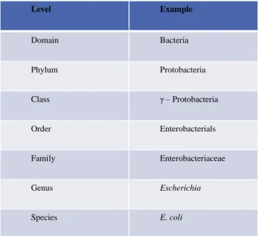
rRNA – known to be a conservative region amongst domain of bacteria. According to definition of taxonomy, it is a systematic way of classifying living organisms that fall under a specific kingdom. For kingdom of bacteria, it is harder to classify an organism as you move to least inclusive class such as order, family, genus and species, the genetic material shared by species within the same genus taxa has a very high percentage of sequence identity. Figure 3.1 below shows the bacterial taxonomy order at level depicts an example of this taxonomy.

Figure 3.1 Bacterial Taxonomy Classification, the focus of this study is on last three taxa, Family, Genus and Species.

There are many applications of genus level identification of bacteria in a sample, especially in metagenomics, infectious disease, and material identification – where a company called Phylagen is trying to map the origin of a product through its manufacturing profile for transparency is global supply chain and to fight counterfeit materials. As metagenomics sample sequencing involves sequencing entire contents of a sample, it can be very difficult to identify a very low

Level Example Domain Bacteria Phylum Protobacteria Class γ – Protobacteria Order Enterobacterials Family Enterobacteriaceae Genus Escherichia Species E. coli

abundance of DNA origin, especially at a genus and species level at which it is more informative and discriminative.

There are many taxonomy classifiers developed with machine learning algorithms such as support vector machine (SVM), random forests, preprocessed nearest neighbor (PLSNN – based on partial least squares) and naïve Bayes [30, 31, 32, 33]. One of the other notable work came from Fioravanti et.al. who developed phylogenetic convolutional neural network (Ph-CNN) for metagenomics dataset [33]. Even though this application is used for metagenomics classification, its main goal is to classify human gut microbiome of Inflammatory Bowel Disease (IBD) patient’s vs healthy controls [33]. This section, however, focuses on classifiers that are based on deep learning models, most of which came after the year 2015. Fiannaca et.al. developed a convolutional neural network (CNN) as well as deep belief network (DBN), whereas Busia et.al. developed a deep neural network (DNN) for this bacterial classification task [34, 35]. In forthcoming sections, Fiannaca et. al.’s study is referred as study 1 and Busia et. al.’s study is referred as study 2.

3.3.1.1 Datasets

Datasets used for bacterial taxonomy classification mainly includes of four main sources 1) complete curated genes of 16S rRNA, 2) whole genome or shot-gun sequencing reads from next generation sequencing (NGS) platforms 3) metagenomics samples and 4) amplicon sequencing reads from primer enhanced libraries. Metagenomics samples are mainly used when environmental samples or community/human gut microbiome samples are being analyzed [33]. Most of metagenomic sample reads available in public dataset, don’t have any corresponding taxonomy classification associated with it, hence normally, a mock metagenomics read datasets are created using popular tools like REAGO [35, 34, 36, 37]. Fiannaca et. al uses this approach to first create a mock dataset and then uses open source tools to isolate reads belonging to 16S gene with 99%

accuracy, mainly for comparisons and testing purposes. The authors of this paper, also create another dataset, called shot-gun (SG) and amplicon (AMP) by downloading over 57788 16S gene sequences from RDP database (dated on 16th September, 2016) by filters using such as length greater than 1200 bps, quality – good , and source – isolate [34, 38]. However, to tackle imbalance dataset, authors limit this dataset by selecting sequences only belonging to Protobacteria Phylum, hence having 1000 sequences from 100 genera and 10 species per genus. The final number of sequences belonged to 3 classes, 20 orders, 39 families, and 100 genera. After selecting these sequences, Grinder was used to generate both shotgun and amplicon sequences with mutations rate with replacement at 3 x 10-3 + 3, 3 x 10-8 x i4, where i is the position of nucleotide [39]. For amplicon sequences, primers for only V3-V4 regions that are approximately 469 bp long combined, were considered, which resulted in 28000 short reads, and losing 86 sequences that didn’t match with the primers used described in [40]. The reasons for choosing V3 was that it has the most amount of single nucleotide polymorphisms (SNPs) and V4 region has been regarded as most discriminatory against V5-V6 for phylogenetic variance [40, 41, 42, 43].

The dataset was obtained from National Center for Biotechnology Information (NCBI) using reference sequence database (RefSeq) to generate the mock reads dataset (reference NCBI). More specifically 18,902 sequences of bacterial 16S rRNA were obtained from the RefSeq BioProjects 33175 and 33317 (downloaded on 27th _{November, 2017). The average length was}

approximately 1455 base pair long, and the sequences varied from 302 to 3600 base pairs [35]. Busia et.al used a multi-length read approach where mock read lengths of 25, 50, 100, 150 and 200 were generated from reference sequence, using a sliding window fashion. In order to get the corresponding taxonomy class information from superkingdom to species level, NCBI Taxonomy Browser was used [44]. The final dataset involved represented 38 phyla, 91 classes, 202 orders,

479 families, 2768 genera(genus) and 13,838 species. Despite of having a lot of number of sequences, for species level there is not a lot of representation for each individual species.

3.3.1.2 Different Methods applied

To prepare short-reads for an input to deep learning architectures such as CNN and RNN, normally, short-reads are converted into one-bit encoding for each of the four bases of A, T, G and C. This creates an array of four bit and replaces 1 to represent each of the above four letters, for example, A is represented as [1,0,0,0], and this is considered one-hot encoded raw vector. Fiannaca et. al. and Busia, et.al both studies represent the four bases in this similar fashion of four-bit array representation. Fiannaca et. all uses k-mer representation to extract features from short-reads that are used in sequence classification tasks [34]. K-mer patterns, occurrences and combinations is heavily used in bioinformatics. There are a few drawbacks of k-mer representations, 1) the positional origin of k-mer in the sequence is not maintained or known and 2) depending on the k in k-mers, meaning the the length of a k-mer, the vector space representation of k-mers suffers from very high dimensionality that can grow exponentially. Fiannaca et. al uses k-mers with size of 3 to 7 [34]. Similar to study 1, study 2 also implemented one-hot encoding for all four bases, A, C, T, G as a four-dimensional vector along with International Union of Pure and Applied Chemistry (IUPAC) ambiguity codes. This dataset is further split into NCBI-0/1/2 for model performance. NCBI-0 contained 90% of the species in each genus by random sampling and by getting second sampling of 90% reads for each selected species in the first sampling. Rest of the 10% reads went to NCBI-1/2. The sequence length for this dataset was set to 100 base pairs. To evaluate the resulting DNN classifier, authors in study 2 created 16S sequences of synthetic community samples from [45, 46, 40]. For these mock communities, the read length selected was 250 base pairs and included 49 bacterial strains and 10 strains from archaea.

3.3.1.3 Main Architectures Used

There are only a few papers that utilizes a true deep learning architecture for bacterial taxonomy classification using 16S rRNA gene or reads belonging to the gene. This review mainly discusses architectures used in aforementioned study 1 and study 2, first uses CNN and DBN as a classifier [34] and second uses DNN (with some convolutions) as a classifier [35]. First published study 1 has a pipeline that starts with classified 16S short-reads, which are then converted into k-mer one-hot encoded vector representation. For learning process, a deep learning architecture both CNN and DBN are deployed and final trained model for each class, order, family and genus are obtained [34]. There is no species level classification utilized since for taxonomy classification genus level classification is highly regarded as a final taxon. In DBN, at least a few Restricted Boltzmann Machine (RBM) are utilized as layers. RBM usually can represent an input in a lower dimensional space to be utilized in following layers [34]. It is an unsupervised learning at first, and then fine-tuning happens using a multilayer perceptron (MLP) and finally a logistic regression layer is utilized as a supervised classifier. Fiannaca et.al uses a derived CNN from LeNet-5 for their architecture design, containing of two convolutional layers, each followed by a max-pooling and a ReLU layers. At the end, two fully-connected layers are utilized with an unspecified classification layer [34].

The authors in study 2, utilizes a DNN structure consisting of depth-wise separable convolutions first introduced by Sifre and Mallat in [47]. The main difference in such convolutions is that they can separate ‘task of learning spatial features’ from ‘integrating information across channels’ [48]. Separable convolutions involve of first depthwise convolutions i of some weight Wd and some input X, which then is an input of a pointwise convolution i of some weight Wp.

by two to three layers of combination of fully connected layer – leaky rectified-linear (LReLU) function – a dropout regularization and a pooling layer. Finally, a softmax classification layer is utilized to compute final probability distribution of over 13,000 species. The network was implemented using TensorFlow library [49]. Batch size was set to 500 reads as an input x compromising of corresponding species class as a label y with ADAM optimizer. The authors in this study 2 also introduced random base-flipping noise in input sequence at different rates between 0% to 16%.

3.3.1.4 Result Comparisons

First study claims to have achieved a 91.3% accuracy at genus lever compared to RDP classifier that achieved a 83.8% accuracy on the same dataset [34]. The authors performed two separate experiments to first comprehend the ideal k-mer size and parameters of networks, and second to find the classifier performance against the RDP classifier. In the first experiment, they observed k-mer of length 7 performed the best with 99% accuracy for class and up to 80% accuracy for genus level in general. However, in comparison to two datasets, the best performing combination was of AMP dataset with CNN classifier, which obtained 91.33% accuracy for about 100 genus taxa compared to SG dataset with CNN classifier obtained 85.50% accuracy. DBN performed well with AMP dataset, achieving about 91.37% accuracy, whereas; with SG dataset it only achieved 81.27% accuracy. In conclusion, the authors conclude that k-mers of the hypervariable regions of V3-V4 used in AMP dataset serve as a more discriminatory feature than k-mers from shotgun sequencing resulting in higher accuracy with CNN classifier.

The second study showed much promising results despite having a very low representation of initial number of sequences belonging to each individual 13,838 species since the authors used 18.907 initial 16S rRNA genes. The results were promising for all taxon especially from

superkingdom to phylum, achieving greater than 95.7% accuracy expect for species taxa where accuracy was 99.9%, 90.0% and 84.4% respectively. However, as real length goes from 200 to 25, for more lower level taxon, such as order, family, genus and species, the accuracies decrease sharply.

3.2 Brief Introduction to Medical Imaging Technology

Over the last few years there have been an exponential growth in number of published papers of machine learning applications in medical image processing. Applications of deep learning especially in medical imaging have been on the rise since 2015. Open medical image data challenges for disease diagnosis, tumor classifications, brain segmentations etc. at popular conferences such as International conference on Medical Image Computing and Computer Assisted Intervention (MICCAI) and on Kaggle online platform have only boosted the popularity of such data analysis amongst the interdisciplinary researchers. Deep learning applications in medical imaging has influenced the research community to such extent that a new international conference named “Medical Imaging with Deep Learning” (MIDL) was initiated in 2018 to accommodate the pace for this research area [50].

3.3 Brief Introduction of Deep Learning applications in Medical Imaging

As indicated in [6], trend in deep learning papers in medical imaging technology is on the rise with most popular model being a CNN due to its ability of being able to learn features from images. However, lately RNN are also being utilized in time-series analysis in medical imaging especially in longitudinal studies that involve of prediction in disease progression. As far as modality of imaging is concerned, the most popular modalities have been MRI and microscopy, in areas of pathology and brain, while segmentation and detection of objects in imaging have topped in area of interest amongst deep learning. Despite of this drastic shift seen in this area, after

2017, there has been an exponential growth, where the number of papers in this field have reached in thousands from hundreds. Some of the core deep learning application areas are discussed further.

3.3.1 Localization/Detection

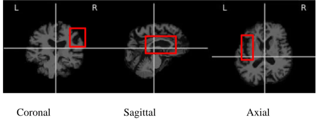
Localization and detection in deep learning is defined as a task of find an object in an image and drawing a bounding box around the entire object as shown in figure 3.2. One of the most crucial application of such task is in self-driving cars where surrounding objects need to be identified and tagged for its position compared to the focal point. In medical imaging, such task is useful for identifying a tumor in brain in space and time or identifying an abnormal cell growth in pathology microscopic images for intervention and planning [6]. In medical imaging, this task normally requires processing of 3D volumetric data. Identifying objects or lesions in images have been one of the cumbersome, tedious yet important part for clinicians.

Coronal Sagittal Axial

Figure 3.2 An example of localization task for brain lesions in Axial, hippocampus detection in sagittal and lesion in coronal sections

Generally, CNN is used to extract features from every pixel with some postprocessing that can identify the possible objects embedded in pixel representation. The bounding box around object is one of the crucial parts of the algorithm in computer vision, which separates it from segmentation task and classification task.

3.3.2 Classification

This was one of the first areas of application of deep learning in medical imaging since CNN’s direct application and popularity for image classification. Earlier in the years, finding a large, balanced and public medical image dataset was an extremely difficult task, hence, most of the applications for clinical detection systems were based on traditional machine learning techniques. After transfer learning algorithms, researchers were able to utilize pre-trained network weights which are trained on millions of generic images, and transfer the learning of features on medical image data classification task despite of having a small dataset. Many studies showed promising results through this, and Litjen’s et.al. described such studies in their review [6].

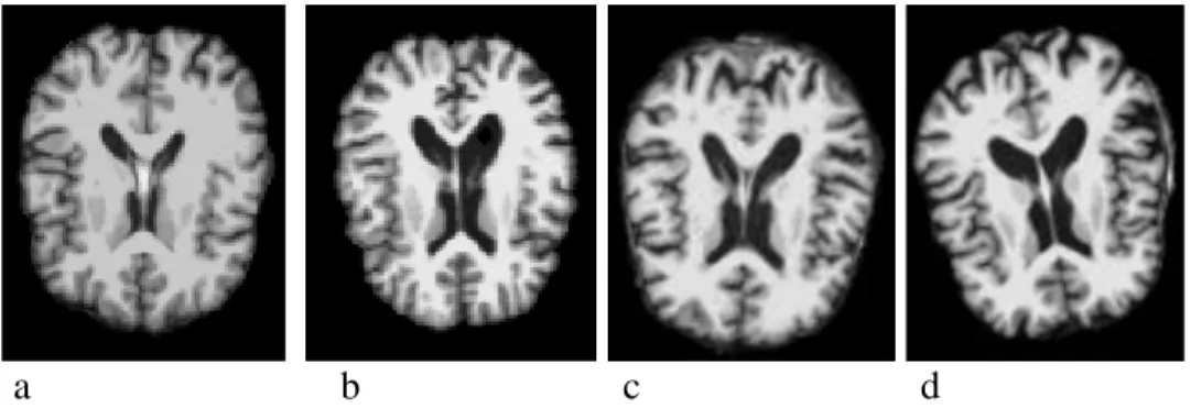
a b c d

Figure 3.3 Classification is achieved by either detecting disease vs normal or by classifying the disease at different stages based on an input image normally a T1-MRI or FDG-PET scan. Above image is from OASIS-3 dataset example of four classes a) Cognitive normal, b) very mild dementia c) mild cognitive dementia and d) Alzheimer’s disease.

There are two types of classification tasks that are popular, first is more superficial or level 1 classification which can identify if an image of a normal patient’s or a disease positive patient. At this level, there is no interest in identifying the disease of the stage of the disease, it is simply asking a question if the image is negative or positive. The deeper classification or level 2 classification as shown in above figure 3.3, where the progression of disease becomes a class or known as label y in neural network prediction outcome. Both areas of classification now have seen

a tremendous growth in research interest. In the earlier days, almost all of the popular CNN networks discussed in chapter 2 were deployed for medical image classification, however, currently most deployed CNN versions have been a 3D CNN, an ensemble or U-net. One such study by Islam and Zhang et.al. achieved a very high accuracy of 93% for normal vs positive Alzheimer’s patient using MRI and FDG- PET scan data from OASIS-2 dataset. The level 1 classification task has been a simpler task to achieve high accuracy; however, level 2 task that required matching is more difficult as disease progression standards varies by physicians to physicians that provide with ground truth values for training of the algorithms.

3.3.3 Segmentation

Segmentation have been one of the most popular application areas in medical imaging. It is used in organ or cell structure segmentation that can serve as clinical features related to area shape in finding abnormalities. Another application of lesion segmentation combines the application of segmentation and detection. More recently, RNNs have become more popular for completing this task, for example, Xie et.al. used a spatial RNN for segmentation in histopathology images, while Stollenga et. al. used 3D LSTM-RNN with convolutional layers. Another popular deep learning architecture for this task has been fCNNs and 2D U-nets in combination with gated recurrent units (GRUs) for 3D segmentation [6].

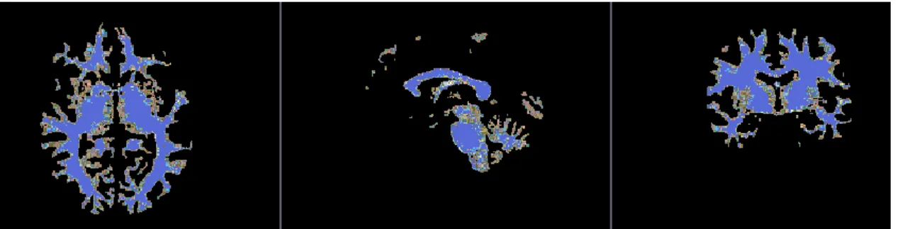
Figure 3.4 Example of OASIS-3 dataset with ground truth of white matter segmentation. Bottom image shows the corresponding of above image for segmented white matter.

Figure 3.4 above illustrates an example of segmentation of white matter in brain axial, sagittal and coronal planes. This segmentation ground truth can differ from physicians to physicians and from different software. Therefore, it is very expensive to minimize this bias by having more than a few medical annotation tasks by physicians that can serve as a good variance for training on deep learning architecture. Hence, the need of more unsupervised learning has been on the rise.

3.3.4 Registration

Lastly, image registration task is spatial alignment of medical images where coordinate transforms is calculated from one medical image to another [6]. Image registration has shown to be beneficial as a preprocessing step in achieving good accuracies of image classification and image segmentation tasks when multi-modal medical image data has been used as an input. One of the ways deep learning techniques are deployed in image registration is to find similarities in two images which then can be optimized further in an iterative fashion. Another way is to predict transformation features using deep regression networks [6]. Nevertheless, in any of the approaches, two way stacked auto-encoders, U-nets and regular CNNs have been the most popular architectures in dealing with image registration tasks.

In [51] one of the more recent tool BIRNet tools that utilizes dual supervised fCNN to solve the image registration in brain MRI images for any of the axial, sagittal, and coronal planes. Also, the authors Fan et.al. uses gap filling, hierarchical loss and multiple sources uses to refine the training processes.

4 16S RIBOSOMAL GENE CLASSIFICATION USING RECURRENT NEURAL

NETWORK AND CONVOLUTIONAL NEURAL NETWORK MODELS

Bacterial 16S ribosomal gene is used to classify bacteria because it consists of both highly conservative region as well as a hypervariable region in its sequence [52, 53]. This hypervariable region serves as a discriminative factor to differentiate bacteria at taxonomic levels. In past, many efforts have been made to correctly identify a bacterial species from environmental samples or human gut microbiome samples, yet this identification and subsequent classification task is challenging. For such bacterial taxonomic classification, several studies in the past have been

performed based on k-mer frequency matching, assembly-based clustering,

supervised/unsupervised machine learning models and a very few studies with deep learning architectures [31, 34, 35]. In this chapter, we study and propose six different deep learning architectures involving Recurrent Neural Networks (RNNs) and Convolutional Neural Networks (CNNs) to classify bacteria at a family, genus and species taxonomic level using approximately 12,900 16S ribosomal DNA sequences. The best classification accuracies achieved are 92%, 86% and 70% at family, genus and species taxonomic level respectively by variants of RNN.

4.1 Introduction

With the rise of refined, cheap and effective sequencing technologies, it is possible to perform targeted sequencing for identification of bacteria obtained from different environmental samples [52]. Due to this phenomenon, a lot more sequencing projects/dataset have been submitted in National Center for Biotechnology Information (NCBI) database and have been made publicly available. Metagenomics studies have lately drawn a lot of attention since it doesn’t require cell cultures in order to characterize bacterial species [53]. Much more standardize approach is yet to

be set for processing such large dataset without creating bias in these analyses. Currently bacterial taxonomic classification tasks depend on read-based sequence matching using tools like mothur and Quantitative Insights Into Microbial Ecology (QIIME) [54, 55]. These tools perform matching of sequences using algorithms involving k-mer frequency, Basic Local Alignment Search Tool (BLAST) and suffix trees. With rise of machine learning algorithms in past decade, various studies emerged involving naïve Bayes approaches such as RDP classifier, hierarchical clustering, random forests and support vector machines (SVM) [31, 34, 35, 38, 56, 57]. To an extent all these studies rely on sequence similarity matching or k-mer frequency counting [38, 56, 31, 57]. Such k-mer based approaches can be limiting as they are independent of a motif position information along with initial sequencing errors/biases which potentially creates noisy input data leading to an inaccurate analysis.

With accessible computational resources and large public data repositories, deep learning techniques are in-demand for classification tasks involving medical image analysis, cancer genomics as well as correcting sequencing errors [58, 59]. There are various kind of neural networks such as the Convolutional Neural Networks (CNNs), the Recurrent Neural Networks (RNNs) and simple Deep Neural Networks (DNNs). While CNNs are generally considered to be a class of feed-forward artificial neural networks in which connections between nodes do not form a cycle and are trained to recognize patterns across the entire spatial domain. Whereas in RNNs, connections between nodes form a directed graph along a temporal sequence allowing this class of neural networks to exhibit temporal dynamic behavior which is highly beneficial while processing sequences, for instance, time-series data. Thus, RNNs are trained to recognize patterns over the time domain. CNNs are normally fixed input size architectures that have found most of their applications to be in the computer vision domain. However, recently scientific community

has shown promising results for natural language processing (NLP) related classification tasks using CNNs. Some of the applications of such NLP related classification tasks involves sentiment analysis, spam detection or topic categorization as CNNs can identify patterns (in form of n-grams) from regular expressions in any text data regardless of their position [60, 61, 62, 63, 64, 65, 66, 67].

4.2 Dataset

The dataset was downloaded from Genomic-based 16S ribosomal RNA Database (GRD), which is a manually curated 16S ribosomal DNA sequences [68]. The dataset has sequences that varies in lengths from 65 to 2900, which means some of the sequences are not complete genes and some of the sequences have more basepairs than 16S rDNA sequence, which normally is ~1500 bp long. The dataset has two separate files, one sequence fasta file, and another metadata file containing tab-delaminated fasta header tag matched to bacterial taxonomy of which corresponding sequences belong to. This study focuses on bacterial classification at Family, Genus and Species levels only since normally Phylum, Class and Order level classification achieves > 99% accuracy in most of the models due to sequences belonging to lesser categories [34, 35]. This dataset had sequences belonging to 272, 840 and 2456 categories for family, genus and species level respectively. For input files, each sequence was first separated with respective family, genus and species category comma separated files. Each file was then further processed to cut each sequence in 100 bp non-overlapping length to compare it with variable full-length sequences (results not included in this study). To ensure each subsequence length is 100, if the last cut fragment is greater than 30 bp, it was then padded with Ns else the fragment was discarded. Ambiguous characters other than ATCG were treated as N for model characters. The sequences were randomly divided in 80% training and 20% testing(validation) dataset. This random split may