A hybrid approach to the problem of class imbalance

(1)

A HYBRID APPROACH TO THE PROBLEM OF CLASS

IMBALANCE

Jeannie Fitzgerald and Conor Ryan

Biocomputing and Developmental Systems Group University of Limerick

Ireland

Abstract: In Machine Learning classification tasks, the class imbalance problemis an important one which has received a lot of attention in the last few years. In binary classification, class imbalance occurs when there are significantly fewer examples of one class than the other. A variety of strategies have been applied to the problem with varying degrees of success. Typically previous approaches have involved attacking the problem either algo-rithmically or by manipulating the data in order to mitigate the imbalance. We propose a hybrid approach which combines Proportional Individualised Random Sampling(PIRS) with two different fitness functions designed to improve performance on imbalanced classification problems in Genetic Programming. We investigate the ef-ficacy of the proposed methods together with that of five different algorithmic GP solutions, two of which are taken from the recent literature. We conclude that the PIRS approach combined with either average accuracy or Matthews Correlation Coefficient, delivers superior results in terms of AUC score when applied to either balanced or imbalanced datasets.

Keywords: Genetic Programming, Binary Classification, Class Imbalance Problem, Over Sampling, Under Sam-pling

1 Introduction

Each day 2.5 quintillion bytes of data are created. This is a relatively recent phenomenon, such that 90% of the data in the world today has been created in the last two years alone [1]. This explosion in data offers tremendous opportunities for knowledge acquisition and decision support, but the potential for unleashing the power of these insights is balanced by several complex challenges. Aside from the problem of handling the sheer volume of data, there is the challenge of identifying those instances which may be interesting or useful, in an environment where such items may be in the minority. From a machine learning perspective, at its simplest, this can be viewed as a binary classification problem.

In binary classification tasks, the class imbalance problem arises where there is a disparity in the number of instances of each class in a particular dataset. Greater disparity makes classification tasks more difficult, as there is an inherent bias towards the class which has greater representation in the dataset. When a machine learning algorithm, designed for general classification tasks, is confronted with significant imbalance, the “intelligent” thing for it to do is to classify all instances as belonging to the majority class. Ironically, it is frequently the case that the minority class is the one which contains the most important or interesting instances. In datasets from the medical domain, for example, it is generally the case that instances which represent malignancy or disease are far fewer than those which do not.

The way in which GP, similar to other approaches which adhere to a paradigm of evolutionary computation is realised: the evolution of a population of individuals over time (generations), means that it facilitates a very flexible and potentially granular approach for tackling this type of problem. We have chosen to investigate a hybrid approach which seeks to influence the learning process at both the individual and population levels, using a strategy which combines sampling and algorithmic techniques. In this work, we propose a new sam-pling technique which we callIndividualised Random Sampling which we combine with Matthews Correlation Coefficient and balanced accuracy.

2 Previous Work

The class imbalance problem is an important one which has generated a lot of interest in the research community in recent years. In general, approaches can be divided between those which tackle the imbalance at the data level, and those which seek an algorithmic solution. There have also been several hybrid techniques proposed which combine aspects of the other two.

(2)

Methods which operate on the data try to repair the imbalance by creating more balanced datasets for training purposes. This is done by under-sampling the majority class or over-sampling the minority class, where the former involves removing some examples of the majority class and the latter is accomplished by adding duplicate copies of minority instances until some predefined measure of balance is achieved. Over or under-sampling may be random in nature [2] or “informed” [3], where in the latter, various criteria are used to determine which instances from the majority class should be discarded. An interesting approach called SMOTE (Synthetic Minority Oversampling Technique) was suggested by Chawla et al. [4] in which rather than over sampling the minority class with replacement they generated new synthetic examples.

At the algorithmic level Joshi et al. [5] modified the well known AdaBoost [6] algorithm so that different weights were applied for boosting instances of each class. Akbani et al. [7] modified the kernel function in a Support Vector Machine implementation to use an adjusted decision threshold. Class imbalance tasks are closely related to cost based learning problems, where misclassification costs are not the same for both classes. Adacost [8] and MetaCost [9] are examples of this approach. See [10–12] for detailed reviews of these and various other approaches found in the literature.

2.1 Genetic Programming (GP)

In the field of GP, much of the work on algorithmic approaches has been undertaken by Bhowan et al. [13–15] in which they have studied the efficacy of a wide range of different fitness functions on various imbalanced data sets. In this work we compare with two of those methods: Correlation Ratiobased fitness, andGeometric Mean based fitness, with which the researchers reported good results. These are described in Sections 4.1.4 and 4.1.5. In other work Patterson and Zhang [16] investigated the use of average accuracy as a fitness function and also a modified version which used the squares of the individual accuracies for each class. Both methods resulted in improved performance on the minority class and a more balanced classification overall.

With regard to sampling approaches in GP, Hunt et al. [17] examined several different sampling approaches including under sampling, over sampling and a combined approach. In each case they maintained equal numbers of instances from both classes in their training set and sampled the majority class with replacement. While they found that the various sampling approaches improved the classification accuracy on the minority class, performance on the majority class decreased. Overall, they reported that the method was not as successful as algorithmic approaches previously suggested by Bhowan et al. [14].

In other work, Doucette and Heywood [18] proposed a Simple Active Learning Heuristic (SALH): a hybrid approach which combined a simplified version of the Random Subset Selection algorithm proposed by Gathercole and Ross [19], together with a modified Wilcoxon-Mann-Whitney statistic. They reported that their hybrid approach compared favourably with several other machine learning algorithms.

3 A Hybrid Approach: Proportional Individualised Random Sampling (PIRS)

with Matthews Correlation Coefficient or Average Accuracy

There several disadvantages associated with the use of over or under sampling strategies for tackling the the class imbalance problem. The obvious disadvantage with under-sampling is that it discards potentially useful data. The main drawback with standard oversampling is that it introduces exact copies of minority instances which may increase the potential for over-fitting. Also, the use of over-sampling increases the size of the dataset, thus adding to the computational cost. Here we propose a sampling approach which we call Proportional Individualised Random Sampling (PIRS) which either eliminates or mitigates these disadvantages.

Firstly, the size of the dataset is exactly the same as the original, so there is no additional computational cost, as is generally the case with random over sampling. Instead, in a new sampling technique, we vary the number of instances of each class maintaining the original size of the dataset. At each generation and for each individual in the population the percentage of majority instances is randomly selected in the range between the percentages of minority (positive) and majority (negative) instances in the original distribution. Then,that particular individual is trained on that percentage of majority instances with instances of the minority class making up the remainder of the data. In both cases, each instance is randomly selected with replacement. For example, in the case of the Yeast1.5 dataset, where 98.5% of the data makes up the majority class and 1.5% the minority, the training data for a given individual will be dividedn percent majority instances where 1.5<=n <= 98.5 andmpercent minority instances, where m= 100−n. In this way, individuals within the

population are trained with different distributions of the data within therange of the original distribution. The benefit of this approach from the under sampling perspective is that while the majority class may not be fully represented at the level of the individual, all of the data for that class is available to the population as a whole. Because all of the available knowledge is spread across the population the system is less likely to suffer from the loss of useful data that is normally associated with under sampling techniques. From the under sampling viewpoint, over-fitting may be less likely as the distribution of instances of each class is varied for

(3)

each individual at every generation. Also, as all sampling is done with replacement, there will be duplicates of negative as well as positive instances.

A useful advantage of our proposed approach is that it is equally applicable to both balanced and unbalanced datasets. Previous work [20] has shown that aside from the consideration of balance in the distribution of instances, the use of random sampling techniques may have a beneficial effect in reducing over-fitting. Thus, we believe that the proposed sampling approach can offer improved performance on a wide range of binary classification tasks, whether a particular dataset is balanced or not. This important proposition was simply addressed by Provost [21] in the invited paper for the AAAI 2000 Workshop on Imbalanced Data Sets ..“isn’t the best research strategy to concentrate on how machine learning algorithms can deal most effectively with whatever data they are given?”.

We combine the PIRS sampling technique with two different fitness functions which are designed to function well with either balanced or unbalanced data: Average Accuracy and Matthews Correlation Coefficient. In Machine Learning, Matthews Correlation Coefficient is widely regarded as a good measure for evaluating the performance of a given model on binary classification tasks, in part because it has fewer inherent biases than some other popular methods [22]. But also, because it is considered suitable for both balanced and imbalanced data sets. Here, rather than using the measure to assess the performance of our model, we investigate its use in the actual evolution of the model by incorporating it as a fitness function as described in Equation 1.

M CC(P) = p (T P ∗T N−F P ∗F N)

(T P +F P)(T P+T N)(F P +F N)(T N+F N) (1) MCC is regarded as a balanced measure of the quality of a binary classifier, which can be used even if the classes are of different sizes. It is, in essence, a correlation coefficient between the observed and predicted binary classifications. MCC returns a value between −1 and +1: where a value of +1 represents a perfect prediction,

a value of 0 no better than random and a value of −1 represents total disagreement between predicted and

observed class labels.

In addition to investigating the use of PIRS with Matthews Correlation Coefficient, we also study the combination of PIRS andaverage accuracy also known asbalanced accuracy which is a well know performance measure used in classification. This method modifies the calculation for overall accuracy to better emphasise the performance oneach class as shown in Equation 2.

AV GA(P) = 0.5∗ T P (T P +F N)+ T N (T N+F P) (2)

4 Experimental Set-up

4.1 Configurations

In much of the literature on binary classification the classes in question are often identified as being positive or negative, where instances of the positive class are usually (but not always) in the minority. This situation is common, for example, in medical diagnosis, where the number of patients with the disease or condition of interest are generally fewer in number than those without the disease. The results of a classifier can be represented by a confusion matrix as shown in table 1. Where TP, TN, FP and FN represent the number of instances which fall into the corresponding category: True Positive, True Negative, False Positive and False Negative.

Table 1: Confusion Matrix

Prediction

Positive Negative

Truth Positive TP FN

Negative FP TN

For the purpose of discussing class imbalance, we are interested in the majority and minority classes, where the majority class corresponds to the negative class and the minority class to the positive class. TP represents the number of minority class instances correctly classified, TN the number of majority class instances correctly classified, FP the number of majority class instances which have been incorrectly classified as belonging to the minority class, and FN the number of minority class instances which have been mis-classified as majority class instances. In describing the various experimental configurations below, we adhere to the standard nomenclature for clarity.

(4)

4.1.1 Standard GP (StdGP)

The fitness measure used for the standard GP configuration is a commonly used measure of “overall” classi-fication accuracy. If a program P correctly classifies all instances, its overall accuracy will be 1. The fitness function for each programP is 1−Accuracy(P), whereAccuracy(P) is as described in Equation 3.

Accuracy(P) = T P+T N

T P +T N+F P +F N (3)

4.1.2 Standard GP withAverage Accuracy (AVGA)

For the second configuration, we use a slight modification of the overall accuracy, which aims to maximise the average of the accuracy over both classes. The fitness function to be minimised is 1−AV GA(P) where

AV GA(P) is described by Equation 2.

4.1.3 GP with Matthews Correlation Coefficient (MCC)

For this configuration we employ a standard GP implementation with the Matthews Correlation Coefficient as the fitness function. This fitness function is described in Section 3 and Equation 1.

4.1.4 GP with Correlation Based Fitness (CORR)

Bhowan et al. [13] proposed a correlation ratio fitness measure to mitigate bias introduced by class imbalance for image classification problems. In this method the correlation ratio is used to measure how well the outputs of a GP Individual for the minority and majority classes areseparated with respect to each other. The higher the correlation ratio achieved by a particular model, the better the classification performance. This fitness function is aimed at evolving solutions that perform equally well on both classes with the minimum loss to the overall classification rate. The correlation ratio ”r” (generalised forM classes) is described in Equation 4.

r(P) = v u u t PM c=1Nc(¯µc−µ¯)2 PM c=1 PN c i=1(Pci−µ¯)2 (4) Where ¯µc is the mean of the outputs of the program for instances of class c, ¯µ is the mean of the program

outputs over all classes, M is the number of classes, N is the number of total instances, Nc is the number of

examples of classc, andPci represent the output of a genetic program classifier P when evaluated on the ith

example belonging to classc. This equation returns a value between 0 and 1, where values closer to 1 indicated better separability.

The researchers also imposed and identity function to guide the evolution such that outputs for instances of the majority class would be greater than zero, and outputs for instances of the minority class would be less than zero. Their final fitness function is shown in Equation 5

Correlation(P) =r+I(¯µminority,µ¯majority) (5)

Where the indicator function, I returns 1 if the mean of the minority and majority observations are positive and negative respectively, and 0 otherwise. Thus, the final fitness function returns a value between 0 and 2 where values closer to 2 represent good fitness, and those nearer to 0, poor fitness.

4.1.5 GP with Geometric Mean based Fitness (GMF)

In other work, Bhowan et al. [14] proposed a fitness function using ageometric mean as shown in Equation 6.

GM F(P) = r T P T P +F N ∗ T N T N+F P (6)

This function has the property that if the number of instances of either class correctly classified is zero, then the geometric mean itself will also be zero, which has the effect of penalising individuals which perform badly on one or other class.

4.1.6 Individualised Random Sampling with Balanced Fitness Function (PIRS-BAL)

In this configuration, we employ the balanced fitness function defined in Equation 2. But we also randomly select training instances to train each individual. The data is randomly selectedwith replacement, varying the proportions of minority and majority class instances. The detail of our sampling technique is as previously described in Section 3.

(5)

Table 2: GP Parameters Parameter Value Strategy Generational Initialisation Ramped half-and-half Selection Tournament Tournament Size 2 Crossover 80 Mutation 20

Initial Min Depth 1 Initial Max Depth 6

Max Depth 17

Function Set + - * /

ERC -5 to +5

Population 500

Max Gen 60

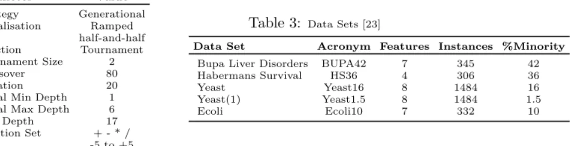
Table 3: Data Sets [23]

Data Set Acronym Features Instances %Minority Bupa Liver Disorders BUPA42 7 345 42 Habermans Survival HS36 4 306 36

Yeast Yeast16 8 1484 16

Yeast(1) Yeast1.5 8 1484 1.5

Ecoli Ecoli10 7 332 10

4.1.7 Individualised Random Sampling with MCC (PIRS-MCC)

In this final experimental configuration we investigate Individualised Random Sampling (PIRS) together with Matthews Correlation Coefficient: an aggregate objective function which represents a particular confusion matrix as a single value. For the PIRS-MCC configuration, we minimise 1−M CC(P) where MCC(P) is as

previously outlined in Equation 1. Here again, the sampling method is as described in Section 3.

4.2 GP Parameters

The Genetic Programming parameters used for this investigation are as described in Table 2 and The datasets used are detailed in Table 3. The yeast and ecoli datasets were originally multi-class datasets. In order to experiment with various levels of class imbalance, we have “collapsed” several of the classes into one to create binary classification tasks. The acronym used for each dataset indicates the % of the minority class in each dataset. In each case we have used two thirds of the available data from training and the remaining one third for test. We undertook 50 runs for each configuration, on each dataset, using identical random seeds for each set of 50 runs.

5 Results and Discussion

For this investigation we have chosen the Area Under the Receiver Operating Curve (AUC) as the primary measure of classification performance. Values for this measure are calculated using the equivalent [24] Wilcoxon-Mann-Whitney statistic. We are also interested in the overall classification accuracy (particularly on test data), performance on the minority and majority classes, the sizes of the evolved classifiers and how early or late in the evolutionary process the best-of-run individual is discovered.

In the following subsections, we detail for each dataset investigated, run statistics for the best of run individuals; the AUC measure, average overall %accuracy on training and test data, best individual %accuracy for training and test data, average%error on the minority and majority classes for both training and test data, the average size in nodes and the average generation in which the best-of-run individual emerged.

To gain a clearer insight as to which method performed best overall we carried out the non parametric Friedman test which is regarded as a suitable test for the empirical comparison of the performance of different algorithms [25]. This resulted in a p-value of 0.003 and indicated that the best performing algorithm in terms of AUC score was PIRS-BAL closely followed by PIRS-MCC as shown in Figure 5.

5.1 BUPA42

The results shown in Table 4 illustrate that the stdGP method which uses the overall accuracy fitness measure performs very poorly on the minority class. The best approach overall is the PIRS-BAL method which combines PIRS with average accuracy. This method delivered a superior AUC measure of 0.80, produced the smallest programs where the best of run individual was discovered earliest in the evolutionary process. It also exhibits an absence of over-fitting, where the average test performance for both the minority and majority classes were actuallybetter than the training results.

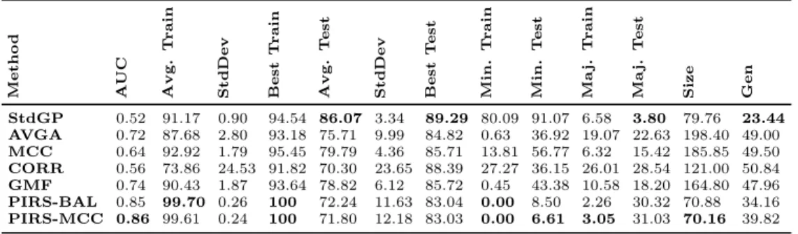
5.2 Ecoli10

Looking at the Ecoli10 results in Table 5 we see that both methods which employed PIRS achieved good AUC scores and performed very well on the minority class, having several runs with perfect classification in the

(6)

AVG CORR GMF GP IRS−B IRS−M MCC 1 2 3 4 5 6 7

Figure 1: Methods ranked from 1 to 7 based on average AUC, where 1 is best and 7 is worst.

Table 4: Performance of best-of-run Trained Individuals on the BUPA42 data.

M e t h o d A U C A v g . T r a in S t d D e v B e s t T r a in A v g . T e s t S t d D e v B e s t T e s t M in . T r a in M in . T e s t M a j. T r a in M a j. T e s t S iz e G e n StdGP 0.74 73.68 1.09 76.32 70.96 2.24 75.44 46.97 51.95 22.85 11.75 213.0 50.50 AVGA 0.80 80.99 1.26 83.33 74.75 3.07 78.95 27.79 42.89 10.22 11.93 88.85 48.22 MCC 0.78 76.22 1.36 78.95 74.03 3.66 78.95 34.02 41.02 16.33 14.02 144.72 54.16 CORR 0.76 66.46 5.06 75.43 70.10 6.64 78.94 31.52 31.79 35.00 28.46 114.25 57.08 GMF 0.69 73.32 1.76 77.19 68.28 4.78 76.31 28.12 36.24 25.62 28.31 161.04 56.28 PIRS-BAL 0.83 65.82 3.78 72.80 76.14 3.31 80.70 41.41 37.89 26.72 13.29 63.48 36.16 PIRS-MCC 0.78 80.66 1.39 84.21 73.91 3.06 78.07 22.23 33.46 17.05 20.52 89.76 48.96

training phase. The GMF and AVGA approaches also achieved good training scores on the minority class, but these did not translate into good test results.

Table 5: Performance of best-of-run Trained Individuals on the Ecoli10 data.

M e t h o d A U C A v g . T r a in S t d D e v B e s t T r a in A v g . T e s t S t d D e v B e s t T e s t M in . T r a in M in . T e s t M a j. T r a in M a j. T e s t S iz e G e n StdGP 0.52 91.17 0.90 94.54 86.07 3.34 89.29 80.09 91.07 6.58 3.80 79.76 23.44 AVGA 0.72 87.68 2.80 93.18 75.71 9.99 84.82 0.63 36.92 19.07 22.63 198.40 49.00 MCC 0.64 92.92 1.79 95.45 79.79 4.36 85.71 13.81 56.77 6.32 15.42 185.85 49.50 CORR 0.56 73.86 24.53 91.82 70.30 23.65 88.39 27.27 36.15 26.01 28.54 121.00 50.84 GMF 0.74 90.43 1.87 93.64 78.82 6.12 85.72 0.45 43.38 10.58 18.20 164.80 47.96 PIRS-BAL 0.85 99.70 0.26 100 72.24 11.63 83.04 0.00 8.50 2.26 30.32 70.88 34.16 PIRS-MCC 0.86 99.61 0.24 100 71.80 12.18 83.03 0.00 6.61 3.05 31.03 70.16 39.82 5.3 HS36

For the HS36 task, once again both PIRS methods produced the best AUC scores, the best minority performance and smallest programs. Again these programs were discovered earlier in the evolutionary process.

5.4 Yeast16

For the Yeast16 dataset, the results in Table 7 show that the CORR fitness function resulted in the best AUC score of 0.83. This method delivered the best accuracy on the minority class and the results were balanced across both classes. PIRS-BAL PIRS-MCC and MCC each had AUC scores of 0.82. MCC had relatively weak accuracy on the minority class but very good results for the majority class. Between PIRS-BAL and PIRS-MCC, the former had the better results on the minority class.

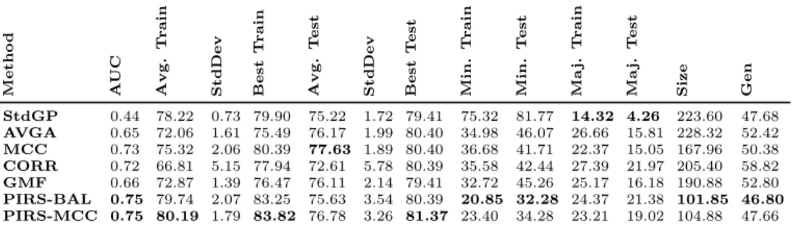
5.5 Yeast1.5

This dataset is the most unbalanced of those tested, and proved to the most difficult from the point of view of minority classification. The results in Table 8 illustrate that StdGP, MCC and CORR achieved relatively

(7)

Table 6: Performance of best-of-run Trained Individuals on the HS36 data. M e t h o d A U C A v g . T r a in S t d D e v B e s t T r a in A v g . T e s t S t d D e v B e s t T e s t M in . T r a in M in . T e s t M a j. T r a in M a j. T e s t S iz e G e n StdGP 0.44 78.22 0.73 79.90 75.22 1.72 79.41 75.32 81.77 14.32 4.26 223.60 47.68 AVGA 0.65 72.06 1.61 75.49 76.17 1.99 80.40 34.98 46.07 26.66 15.81 228.32 52.42 MCC 0.73 75.32 2.06 80.39 77.63 1.89 80.40 36.68 41.71 22.37 15.05 167.96 50.38 CORR 0.72 66.81 5.15 77.94 72.61 5.78 80.39 35.58 42.44 27.39 21.97 205.40 58.82 GMF 0.66 72.87 1.39 76.47 76.11 2.14 79.41 32.72 45.26 25.17 16.18 190.88 52.80 PIRS-BAL 0.75 79.74 2.07 83.25 75.63 3.54 80.39 20.85 32.28 24.37 21.38 101.85 46.80 PIRS-MCC 0.75 80.19 1.79 83.82 76.78 3.26 81.37 23.40 34.28 23.21 19.02 104.88 47.66

Table 7: Performance of best-of-run Trained Individuals on the Yeast16 data.

poor results in this respect: correctly classifying fewer than half of the minority examples. In contrast, the PIRS-BAL method produced relatively good results on both classes and had the highest AUC score.

Table 8: Performance of best-of-run Trained Individuals on the Yeast1.5 data.

6 Conclusion

Looking at trends in the reported results it is clear that the overall accuracy measure commonly used for classification tasks in GP is inferior to all of the other methods investigated, performing poorly even on the relatively balanced Bupa42 dataset. In contrast, both of the PIRS methods performed well on all of the tasks, under each of the criteria examined: either PIRS-BAL or PIRS-MCC achieved or shared the best AUC score for all but one of the tasks, each delivered competitive results for overall accuracy on training and test data, and for both minority and majority classification. These configurations also produced the smallest trees on average, and the best-of-run individuals were discovered on average earlier in the evolutionary process.

These results suggest that Individualised Random Sampling combined with a fitness function that is designed to operate well with unbalanced datasets can deliver superior results onboth balanced and unbalanced data.

Acknowledgement: This work has been supported by the Science Foundation of Ireland. Grant No. 10/IN.1/I3031.

References

[1] Zikopoulos, P. et al., Understanding big data: Analytics for enterprise class hadoop and streaming data, McGraw-Hill Osborne Media, 2011.

(8)

[3] Kubat, M. et al., Addressing the curse of imbalanced training sets: one-sided selection, in MA-CHINE LEARNING-INTERNATIONAL WORKSHOP THEN CONFERENCE-, pages 179–186, MOR-GAN KAUFMANN PUBLISHERS, INC., 1997.

[4] Chawla, N. V., Bowyer, K. W., Hall, L. O., and Kegelmeyer, W. P., arXiv preprint arXiv:1106.1813 (2011). [5] Joshi, M. V., Kumar, V., and Agarwal, R. C., Evaluating boosting algorithms to classify rare classes: Com-parison and improvements, inData Mining, 2001. ICDM 2001, Proceedings IEEE International Conference on, pages 257–264, IEEE, 2001.

[6] Freund, Y. and Schapire, R. E., Experiments with a new boosting algorithm, inThirteenth International Conference on Machine Learning, pages 148–156, San Francisco, 1996, Morgan Kaufmann.

[7] Akbani, R., Kwek, S., and Japkowicz, N., Applying support vector machines to imbalanced datasets, in Machine Learning: ECML 2004, pages 39–50, Springer, 2004.

[8] Fan, W., Stolfo, S. J., Zhang, J., and Chan, P. K., Adacost: misclassification cost-sensitive boosting, in MACHINE LEARNING-INTERNATIONAL WORKSHOP THEN CONFERENCE-, pages 97–105, Cite-seer, 1999.

[9] Domingos, P., Metacost: a general method for making classifiers cost-sensitive, inProceedings of the fifth ACM SIGKDD international conference on Knowledge discovery and data mining, pages 155–164, ACM, 1999.

[10] Kotsiantis, S. et al., GESTS International Transactions on Computer Science and Engineering30(2006) 25.

[11] He, H. and Garcia, E. A., Knowledge and Data Engineering, IEEE Transactions on21(2009) 1263. [12] SIGKDD Explor. Newsl.6(2004).

[13] Bhowan, U., Zhang, M., and Johnston, M., Genetic programming for image classification with unbalanced data, in Proceeding of the 24th International Conference Image and Vision Computing New Zealand, IVCNZ ’09, pages 316–321, Wellington, 2009, IEEE.

[14] Bhowan, U., Johnston, M., and Zhang, M., Differentiating between individual class performance in genetic programming fitness for classification with unbalanced data, inEvolutionary Computation, 2009. CEC’09. IEEE Congress on, pages 2802–2809, IEEE, 2009.

[15] Bhowan, U., Johnston, M., and Zhang, M., Evolving ensembles in multi-objective genetic programming for classification with unbalanced data, in Proceedings of the 13th annual conference on Genetic and evolutionary computation, pages 1331–1338, ACM, 2011.

[16] Patterson, G. and Zhang, M., Fitness functions in genetic programming for classification with unbalanced data, inProceedings of the 20th Australian Joint Conference on Artificial Intelligence, edited by Orgun, M. A. and Thornton, J., Lecture Notes in Computer Science, pages 769–775, Gold Coast, Australia, 2007, Springer.

[17] Hunt, R., Johnston, M., Browne, W., and Zhang, M., Sampling methods in genetic programming for clas-sification with unbalanced data, inAI 2010: Advances in Artificial Intelligence, pages 273–282, Springer, 2011.

[18] Doucette, J. and Heywood, M., Gp classification under imbalanced data sets: Active sub-sampling and auc approximation, inGenetic Programming, edited by ONeill, M. et al., volume 4971 ofLecture Notes in Computer Science, pages 266–277, Springer Berlin Heidelberg, 2008.

[19] Gathercole, C. and Ross, P., Dynamic training subset selection for supervised learning in genetic program-ming, inParallel Problem Solving from NaturePPSN III, pages 312–321, Springer, 1994.

[20] Liu, Y. and Khoshgoftaar, T., Reducing overfitting in genetic programming models for software qual-ity classification, inHigh Assurance Systems Engineering, 2004. Proceedings. Eighth IEEE International Symposium on, pages 56–65, IEEE, 2004.

[21] Provost, F., Learning with imbalanced data sets, inInvited paper for the AAAI2000 Workshop on Imbal-anced Data Sets, 2000.

[22] Powers, D., Journal of Machine Learning Technologies2(2011) 37. [23] Frank, A. and Asuncion, A., UCI machine learning repository, 2010.

[24] Yan, L., Dodier, R., Mozer, M. C., and Wolniewicz, R., Optimizing classifier performance via the wilcoxon-mann-whitney statistics, in Proceedings of the 20th international conference on machine learning, pages 848–855, Citeseer, 2003.

[25] Gerevini, A., Saetti, A., and Serina, I., An experimental study based on Friedman’s test of some local search techniques for planning, pages 59–68.