Nonparametric predictive inference for diagnostic test thresholds

(1)

Durham E-Theses

Nonparametric predictive inference for diagnostic test

thresholds

ALABDULHADI, MANAL,HAMAD,M

How to cite:

ALABDULHADI, MANAL,HAMAD,M (2018) Nonparametric predictive inference for diagnostic test thresholds, Durham theses, Durham University. Available at Durham E-Theses Online:

http://etheses.dur.ac.uk/12538/ Use policy

The full-text may be used and/or reproduced, and given to third parties in any format or medium, without prior permission or charge, for personal research or study, educational, or not-for-prot purposes provided that:

• a full bibliographic reference is made to the original source

• alinkis made to the metadata record in Durham E-Theses

• the full-text is not changed in any way

The full-text must not be sold in any format or medium without the formal permission of the copyright holders. Please consult thefull Durham E-Theses policyfor further details.

(2)

(3)

Nonparametric predictive inference

for diagnostic test thresholds

Manal H. Alabdulhadi

A thesis presented for the degree of

Doctor of Philosophy

Department of Mathematical Sciences

Durham University

United Kingdom

March 2018

(4)

for diagnostic test thresholds

Manal H. Alabdulhadi

Submitted for the degree of Doctor of Philosophy

March 2018

Abstract

Nonparametric Predictive Inference (NPI) is a frequentist statistical method that is explicitly aimed at using few modelling assumptions, with inferences in terms of one or more future observations. NPI has been introduced for diagnostic test accuracy, yet mostly restricting attention to one future observation. In this thesis, NPI for the accuracy of diagnostic tests will be developed for multiple future observations. The present thesis consists of three main contributions related to studying the accuracy of diagnostic tests. We introduce NPI for selecting the optimal diagnostic test thresholds for two-group and three-group classification, and we compare two diagnostic tests for multiple future individuals.

For the two- and three-group classification problems, we present new NPI approaches for selecting the optimal diagnostic test thresholds based on multiple future observations. We compare the proposed methods with some classical methods, including the two-group and three-group Youden index and the maximum area (volume) methods. The results of simulation studies are presented to investigate the predictive performance of the proposed methods along with the classical methods, and example applications using data from the literature are used to illustrate and discuss the methods.

NPI for comparison of two diagnostic tests is presented, assuming the tests are applied on the same individuals from two groups, namely healthy and diseased individuals. We also introduce weights to reflect the relative importance of the two groups.

(5)

Declaration

The work in this thesis is based on research carried out in the Department of Mathematical Sciences at Durham University. No part of this thesis has been submitted elsewhere for any degree or qualification.

“The copyright of this thesis rests with the author. No quotation from it should be published without the author’s prior written consent and information derived from it should be acknowledged.”

(6)

Alhamdullilah, Allah my God, I am truly grateful for the countless blessings you have bestowed on me generally and in accomplishing this thesis especially.

My sincere gratitude and thanks go to my supervisors Prof. Coolen and Dr. Tahani Coolen-Maturi for their unlimited support, expert advice and guidance. I really appreciate their patience, kindness and invaluable suggestions with immense knowledge. I am very grateful that I have great supervisors.

My special thanks to my husband Abdullah for being very supportive and my lovely children for understanding that my work kept me very busy. I am internally grateful to my mother for all her unlimited love and prayers and all my brothers and sisters for encouraging and believing.

I would like to thank the sponsors and supporters of my study, Saudi Arabian Cultural Bureau in London, the Ministry of Higher Education in Saudi Arabia and Qassim University.

Many thanks to the Durham University for offering an enjoyable academic atmosphere and for the facilities that have enabled me to study smoothly.

Also, I would like to thank Prof. Sarafidis for providing the interleukin-6 (IL-6) data [61], and Prof. Nakas for providing the n-acetyl aspartate over creatine (NAA/Cr) data [54].

(7)

Chapter 1 Introduction

Diagnostic tests are often used to differentiate patients between two states, healthy and diseased. The results of the diagnostic test may take two values (binary tests), or real values (continuous tests), or a value in a finite number of ordered categories (ordinal tests) [59]. The focus in this thesis is on tests that yield real-valued results.

Assessing the accuracy of diagnostic tests is crucial in many application areas in-cluding medicine and health care. The receiver operating characteristic (ROC) curve is a useful tool to assess the diagnostic test accuracy, and the area under the ROC curve (AUC) is often used as a single global measure of the overall performance of the

dia-gnostics test. For medical applications, it is important to select an appropriate threshold, or differentiation value, such that a person is assessed to be diseased or healthy, depend-ing on ehether their corresponddepend-ing diagnostic test result is greater than the threshold value or not. Therefore, threshold selection methods have been an active field of study [11, 35, 47, 72]. Several methods for selecting thresholds are based on the ROC curve, including the Youden index [33, 72], closest-to-(0,1) [11, 65], maximum area [47] methods and other methods as discussed by Greiner et al. [35].

In this thesis, we introduce a nonparametric predictive approach, called NPI, for selecting the optimal threshold of a diagnostic test, where the inferences focus on future observations. The NPI method uses a direct predictive method to select an optimal threshold, focusing on a limited number of future individuals. NPI is a frequentist

(10)

statistical method that is explicitly aimed at using few modelling assumptions, enabled through the use of lower and upper probabilities to quantify uncertainty. NPI has been introduced for many application areas where the predictive nature of this method plays an important role, including reliability, survival analysis, operations research and finance. Restricting attention to one future observation, NPI has been developed for diagnostic test accuracy considering different types of data. For example, Coolen-Maturi et al. [25] introduced NPI for diagnostic test accuracy with binary data, while Elkhafifi and Coolen [32] presented NPI for diagnostic tests with ordinal data. Coolen-Maturi et al. [24, 26] proposed NPI for two- and three-group ROC analysis with continuous data. The results in [32] have been generalised by Coolen-Maturi [21] for three-group ROC analysis with ordinal data. Recently, Coolen-Maturi [22] considered NPI for scenarios where two or more diagnostic tests are combined in order to improve the overall accuracy.

This thesis develops a new NPI approach, based on multiple future individuals, for selecting the optimal diagnostic test threshold for the two-group scenario and also for selecting the two thresholds needed in a three-group scenario. We focus on the two- and three-group classification problems which are the most used in practice. However, the proposed NPI method is straightforward to generalise for a disease withk groups (stages), as will be briefly mentioned in Section 3.8, the concluding remarks.

Classical methods often focus on estimation rather than prediction. The end goal of studying the accuracy of diagnostic tests is to apply these tests on future patients. Thus, it is of interest to consider the use of a predictive inference method. Another issue would be the validity of the underlying assumptions required by some of these classical methods, which are often difficult to justify in practice.

The important difference of the NPI approach compared with the alternatives in the literature is that the inferences are explicitly in terms of a given number of future individuals. In this thesis, we will show that the number of future individuals considered might influence the choice of the optimal thresholds. If one should make a decision for a predetermined number of future patients, the direct prediction of NPI-based inferences in terms of m patients is clearly attractive. We compare our proposed methods with some

(11)

1.1. Accuracy of diagnostic tests 3

empirical classical methods, including the empirical Youden index and maximum area methods, as these methods also take only few model assumptions.

This chapter is organised as follows. Section 1.1 presents an introduction to the concepts of the accuracy of diagnostic tests. Section 1.2 introduces methods in the literature for establishing the thresholds. In Section 1.3, we provide a brief introduction to NPI. A detailed outline of this thesis is given in Section 1.4.

1.1 Accuracy of diagnostic tests

In two-group classification, accuracy of a diagnostic test is determined by the ability of a test to distinguish between healthy and diseased individuals. Measuring the accuracy of diagnostic tests is an important goal in medical research. Parametric and nonparametric approaches have been introduced for accuracy of diagnostic tests [59, 73]. Test outcomes can be either binary, continuous or ordinal. The focus in this thesis is on continuous diagnostic tests. Let Y be a continuous random quantity representing the outcome of a diagnostic test. Studying a suitable choice of a value of c, called threshold, is the main objective for the accuracy of diagnostic tests. We assume through this thesis that for a specific value of a threshold c ∈ _R, the test result indicates disease if Y > c (‘positive’ test results), and if Y ≤ c the test result indicates non-disease (‘negative’ test results) [59]. Sensitivity (Sn) of a diagnostic test is the probability of a positive test result for an individual with the disease, it is also known as True Positive Fraction (TPF). Specificity (Sp) is the probability of a negative test result for an individual without the disease [59]. A diagnostic test is considered ideal if it has both sensitivity and specificity equal to one [59]. The False Positive Fraction (FPF) is the probability of a positive test result for an individual without the disease, so FPF=1−Sp.

Let X be used to refer to the test result for the healthy group and let Y be used to refer to the test result for the diseased group, and let nx and ny be the numbers of

(12)

corresponding to the threshold cbe FPF(c) and TPF(c), respectively, so

T P F(c) = P[Y > c] (1.1)

F P F(c) = P[X ≥c] (1.2)

The Receiver Operating Characteristic (ROC) curve plots TPF(c) versus FPF(c) over all possible diagnostic thresholdsc∈_R. The ROC curve has become a popular statistical tool for assessing the accuracy of a diagnostic test. The ROC curve can be defined as

ROC ={(F P F(c), T P F(c)), c ∈(−∞,∞)} (1.3)

A perfect diagnostic test completely distinguishes between healthy and diseased individuals for a particular thresholdc?, so FPF(c?) = 0 and TPF(c?) = 1. In contrast, the diagnostic test has no ability to separate individuals with and without disease if FPF(c)=TPF(c) for all c∈_R[59].

The ROC curve depends on the distributions ofX andY, however these distributions are usually unknown. A nonparametric empirical approach has been introduced for estimating the ROC curve for a diagnostic test with continuous results [59]. This approach is commonly used due to its flexibility to adjust entirely to the available data [59, 73]. The corresponding ROC curve is called the empirical ROC curve.

To introduce the empirical ROC curve, we use the following notation. Suppose that we have test data onnx individuals from a healthy group andny individuals from a disease

group, denoted by {xj, j = 1, ..., nx} and {yi, i = 1, ..., ny}, respectively. Assume that

these two groups are fully independent, in the sense that any information about measure-ments on individuals in one group does not contain any information about measuremeasure-ments on individuals in the other group. For the empirical ROC approach, these observations for both groups are assumed to be realisations of random quantities that are identically distributed as X for the healthy group, and as Y for the disease group. The empirical ROC curve is defined by [59]

(13)

1.2. Methods for selection of a threshold 5 with T P Fe(c) = Pny i=11[yi > c] ny (1.5) F P Fe(c) = Pnx j=11[xj ≥c] nx (1.6)

where 1[A] is the indicator function which is equal to 1 if A is true and 0 otherwise. The area under the ROC curve, AUC, is a global measure of the overall ability of the diagnostic test to distinguish among those individuals with and without disease, which has been widely studied in the literature [42, 59, 73]. It is equal to the probability that a randomly selected individual from the diseased group has a test result that is higher than that of a randomly chosen individual from the healthy group, so P[Y > X] [59]. The maximum possible value of the AUC is 1, which indicates an ideal test, and AUC= 0.5 indicates an uninformative test [59, 73]. Pepe [59] and Zhou et al. [73] presented overviews of statistical methodology for diagnostic test accuracy and ROC curve, considering parametric and nonparametric methods of inference on the ROC curve. The ROC curve has been applied in a variety of areas such as medical imaging and radiology [48], credit scoring [9], psychiatry [40] and epidemiology [3].

1.2 Methods for selection of a threshold

To completely define a diagnostic test, selecting the optimal threshold is needed such that the test provides good differentiation of the individuals with and without the disease. Methods for the selection of the optimal threshold based on the ROC analyses have been discussed by Greiner et al. [35] and Schäfer [62]; one of these methods is to maximise the Youden index (YI) [33, 72]. Formally, the Youden index is defined as

YI = max

c {Sn(c) +Sp(c)−1} (1.7)

Geometrically, YI represents the maximum vertical distance between the ROC curve and the diagonal line. The empirical estimate of the Youden index (EYI) is given by

EYI(c) = 1 nx nx X i=1 1{xi ≤c}+ 1 ny ny X j=1 1{yj > c} −1 (1.8)

(14)

where perfect separation of the two groups results in EYI= 1 whereas complete overlap yields EYI= 0 [64].

In medical applications, the Youden index is presented as a useful measure for evalu-ating the diagnostic test procedures. For example, Aoki et al. [3] identified the optimal threshold level of serum pepsinogens for gastric cancer screening using the Youden index. They suggested that the Youden index is useful for identifying the optimal threshold level of serum pepsinogens for gastric cancer screening. Pekkanen and Pearce [58] examined the assessment between bronchial hyperresponsiveness (BHR) and symptom questionnaires of discriminating between asthma and nonasthma by computing the Youden index. The results showed that the symptom questionnaires have a higher Youden index, which could be considered more accurate than BHR. Demir et al. [30] applied the Youden index to measure and compare the assessment of eight discrimination indices in differentiating between thalassemia and iron deficiency anemia (IDA). First, they calculated eight dis-crimination indices in a number of patients with IDA and a number of patients with thalassemia, then they applied the Youden index for each index to determine which is the best for differentiating thalassemia from IDA. The Youden index was shown to be useful to obtain accurate indices in differentiating thalassemia from IDA. Jalali and Rezaie [41] compared the predicting pressure ulcer risk (PrUs) validity of 4 commonly used PrUs assessment tools using the Youden index as measure of validity between them.

There is a recognizable large body in literature of the Youden index, which addresses other issues such as the estimation of the Youden index and its optimal threshold [33, 43, 50, 63, 64]. This is not directly related to our work.

Another approach for establishing the optimal threshold is the closest-to-(0,1) method (MD). This method selects the optimal threshold that corresponds to the point on the curve closest to (0,1) (i.e. the point closest to perfection with Se(c) = 1 and Sp(c) = 1). The optimal threshold is the value that minimises the distance between a point on the curve and (0,1) point. This method can be found mathematically by

MD = min

c {

q

(15)

1.2. Methods for selection of a threshold 7

Perkins and Schisterman [60] discussed a comparison of optimal thresholds selected by this method and the Youden index method. They recommend the use of the Youden index as it offers clear clinical meaning in terms of the probability of correct classification rate. In the literature, the closest-to-(0,1) method has received little attention compared to the Youden index [60].

Recently, Liu [47] proposed an alternative to these methods based on the concept of the area under the ROC curve (AUC), which is the maximum area method (MA). This method defines the optimal threshold as the point that maximising the product of specificity and sensitivity, given by

MA = max

c {Sp(c)×Sn(c)} (1.10)

Liu [47] also discussed a comparison of optimal thresholds selected by this method, the Youden index and the closest-to-(0,1) methods, via a simulation study. The maximum area criterion has a simple and more meaningful maximising function, which evaluates the classification accuracy of binary classification at thresholdc. The empirical estimator for the maximum area method (EMA) is given by

EMA(c) = 1 nx nx X i=1 1{xi ≤c} × 1 ny ny X j=1 1{yj > c} (1.11)

Several other approaches for selecting the optimal threshold based on the ROC curve are discussed by [35, 59, 62, 66]. For example, Unal [66] proposed an approach called Index of Union (IU). In this method the value of AUC is computed first, then we search for a threshold c from the coordinates of the ROC curve whose specificity and sensitivity values are simultaneously very close or equal to the value of AUC. Mathematically, the IU method can be defined by the following equation

IU = min

c (|Se(c)−AU C|+|Sp(c)−AU C|) (1.12)

such that the optimal threshold ccan be found by minimising the IU(c) function [66]. A different method for the optimal threshold selection, which is not based on the ROC curve, employs the use of a maximally selected statistics that maximises a measure of difference

(16)

among the two groups [10, 39, 49]. For example, the minimum P value method (min P) presented by Miller and Siegmund [49], defines the optimal threshold that maximises the standard chi-square statistic with one degree of freedom. In Section 2.5 we will compare our proposed NPI method with the EYI method, Equation (1.7), and EMA method, Equation (1.11), since both methods also take only few model assumptions. It is of interest to compare our NPI approach with, for example, IU and min P methods, but we leave that for further research.

1.3 Nonparametric Predictive Inference

1.3.1 A brief introduction

Nonparametric Predictive Inference (NPI) is a frequentist statistical framework based on Hill’s assumption A(n) [37], which yields direct probabilities for one or more future

observations, based on n observations for related random quantities. A(n) does not

assume anything else and it can be considered as a post-data assumption related to exchangeability. Inferences based on A(n) are nonparametric and predictive, and can be

considered appropriate if there is hardly any information or knowledge about the random quantities of interest, other than thenobservations [38]. Such inferences based on limited knowledge have also been called ‘low structure’ predictive inferences [34].

The assumption A(n) partially specifies a predictive probability distribution for one

future observation as follows. Suppose that X1, . . . , Xn, Xn+1 are continuous, real-valued

and exchangeable random quantities. Suppose that the ordered observations ofX1, . . . , Xn

are denoted byx1 < x2 < ... < xn, and definex0 =−∞andxn+1 =∞for ease of notation

(or x0 = 0 when dealing with non-negative random quantities). We assume that ties do

not occur between the data observations; ties can be dealt with by assuming that tied observations differ by small amounts, a common approach to break ties in statistics [38]. These n observations partition the real-line into n+ 1 intervals Ij = (xj−1, xj), for

(17)

1.3. Nonparametric Predictive Inference 9

likely to fall in any of these intervals with probability _n₊₁1 [14], for each j = 1, . . . , n+ 1, P(Xn+1 ∈Ij) =

1

n+ 1 (1.13)

NPI has been introduced as predictive methodology, based only on the A(n) assumption.

It is important to emphasize that no further assumptions are made on the distribution of probability 1

n+1 within an intervalIj. In NPI uncertainty is quantified by lower and upper

probabilities for events of interest. Augustin and Coolen [6] introduced predictive lower and upper probabilities based on A(n), which are in line with De Finetti’s fundamental

theorem of probability [29]. The lower probabilityP(.) and upper probability P(.) for the event Xn+1 ∈B withB ⊂R, based on the intervalsIj = (xj−1, xj) for j = 1,2, . . . , n+ 1,

created by n real-valued non-tied observations, and the assumption A(n), are given by

P(Xn+1 ∈B) = 1 n+ 1 n+1 X j=1 1{Ij ⊆B} (1.14) P(Xn+1 ∈B) = 1 n+ 1 n+1 X j=1 1{Ij ∩B 6=∅} (1.15)

The lower probability (1.14) is achieved by taking only probability mass into account that is necessarily within B, which is only the case for the probability mass 1

n+1 per interval Ij

if this interval is completely contained withinB. The upper probability (1.15) is achieved by taking all the probability mass into account that could possibly be within B, which is the case for the probability mass _n₊₁1 , per interval Ij, if the intersection of Ij and B is

non-empty. NPI has strong consistency properties in the theory of interval probability [6, 69], and it never leads to results that are in conflict with inference based on empirical distributions.

NPI has been introduced for a variety of data types, NPI for multinomial data with an unknown number of unordered categories was presented by Coolen and Augustin [15] and Baker [7]. Elkhafifi and Coolen [32] presented NPI for ordinal data, based on a latent variable representation with the categories represented by intervals on the real line to reflect the known ordering of the categories. NPI for right-censored data was introduced by Coolen and Yan [19, 20]. In Chapters 2 and 3, we apply NPI for future order statistics as presented by Coolen et al. [16] and Alqifari [2], and in Chapter 4 we apply NPI for

(18)

Bernoulli data introduced by Coolen [13].

1.3.2 NPI for future order statistics

In Section 1.3 NPI was only introduced for one future observation, but it can also be generalized for multiple future observations, where we are interested in m ≥ 1 future observations, Xn+i for i = 1, . . . , m. It is important to emphasize that the future

ob-servations Xn+i are assumed to derive from the same data collection process as the n

data observations. We link the data and future observations via Hill’s assumption A(n)

[37], or more precisely, via consecutive application of A(n), A(n+1), . . . , A(n+m−1), we refer

to these all together as A(.), which can be considered as a post-data version of a finite

exchangeability assumption for n+m random quantities. A(.) implies that all possible

orderings of the n data observations and the m future observations are equally likely, where the n data observations are not distinguished among each other, and neither are the m future observations. LetSj = #{Xn+i ∈Ij, i= 1, . . . , m}, then assuming A(.) we

have [16] P( n+1 \ j=1 {Sj =sj}) = n+m n !−1 (1.16) for any non-negative integerssj withPnj=1+1sj =m. Equation (1.16) implies that all

_n₊_m

n

orderings of m future observations among the n observations are equally likely.

The probability distribution of a single order statistic of m future observations is important in this thesis which will be used in Chapters 2 and 3. LetX(r), forr = 1, . . . , m,

be the r-th ordered future observation, so X(r) =Xn+i for one i= 1, . . . , mand X(1) <

X(2) < . . . < X(m). The following probabilities are derived by counting the relevant

orderings, and hold for j = 1, . . . , n+ 1 andr= 1, . . . , m[16]

P(X(r) ∈Ij) = j+r−2 j−1 ! n−j+ 1 +m−r n−j+ 1 ! n+m n !−1 (1.17)

For this event NPI provides a precise probability, as each of the n+_nm equally likely orderings of n past and m future observations has the r-th ordered future observation

(19)

1.3. Nonparametric Predictive Inference 11

in precisely one interval Ij [16]. Generally, consider the event X(r) ∈ B, where B ⊂ R.

NPI provides bounds for the probability for such an event, where the maximum lower bound and minimum upper bound are the lower and upper probabilities, respectively [5, 6, 68, 69]. Following Equations (1.14) and (1.15) in Section 1.3, we can derive the lower and upper probabilities

P(Xr ∈B) = n+1 X j=1 1{Ij ⊆B}P(X(r) ∈Ij) (1.18) P(Xr ∈B) = n+1 X j=1 1{Ij ∩B 6=∅}P(X(r) ∈Ij) (1.19)

The event that the number of future observations in an interval (xa, xb), with 1 ≤

a < b≤n+ 1 and denoted by Sm

a,b, is greater than or equal to a particular value v ∈N,

has the following precise probability [2],

P(S_a,bm ≥v) = m X i=v n+m n !−1 b−a−1 +i i ! n−b+a+m−i m−i ! (1.20)

Equation 1.20 will be used in Chapter 3.

1.3.3 NPI for Bernoulli quantities

Coolen [13] presented NPI for Bernoulli quantities, which is based on theA(.) assumption,

for m future observations given n observed values, and a latent variable representation of Bernoulli quantities represented as observations on the real line, with a threshold such that observations to one side are successes and to the other side failures. Suppose that there is a sequence ofn+mexchangeable Bernoulli trials, each with ‘success’ and ‘failure’ as possible outcomes, and data consisting of s successes in n trials. Let Y₁n denote the random number of successes in trials 1 to n; then a sufficient representation of the data for NPI is Y₁n = s, due to assumed exchangeablility of all trials. Let Y_nn₊₁+m denote the random number of successes in trials n+ 1 to n+m. Coolen and Coolen-Schrijner [18] presented the lower and upper probabilities for events Y_nn₊₁+m ≥ y and Y_nn₊₁+m < y. The upper probabilities for these events are as follows. For y ∈ {0,1, ..., m} and 0< s < n,

(20)

P

(

Y

_nn₊₁+m

≥

y

|

Y

₁n

=

s

) =

n+_nm−1 " s+y s n−s+m−y n−s

+

Pm l=y+1 s+l−1 s−1 n−s+m−l n−s # (1.21) and for y ∈ {1, ..., m+ 1} and 0< s < n,

P

(

Y

nn+1+m

< y

|

Y

1n

=

s

) =

_n₊_m n −1 " _n₋_s₊_m n−s

+

y−1 P l=1 _s₊_l₋₁ s−1 _n₋_s₊_m₋_l n−s # (1.22)

The corresponding lower probabilities can be derived via the conjugacy property [13], P(Y_nn₊₁+m ≥y|Yn

1 =s) = 1−P(Y

n+m

n+1 < y|Y1n =s)

P(Y_nn₊₁+m < y|Y₁n =s) = 1−P(Y_nn₊₁+m ≥y|Y₁n =s)

For m= 1, the two non-trivial values of these upper probabilities are P(Y_nn₊₁+1 ≥1|Yn

1 =

s) = (s+ 1)/(n+ 1) and P(Y_nn₊₁+1 <1|Yn

1 =s) = (n−s+ 1)/(n+ 1).

If the observed data are all successes, so s =n, or all failures, so s = 0, then these upper probabilities are, for all y∈ {0,1, ..., m},

P(Y_nn₊₁+m ≥y|Y₁n=n) = 1, P(Y_nn₊₁+m ≥y|Yn 1 = 0) = (n+m−y n ) (n+m n ) , and for ally ∈ {0,1, ..., m+ 1},

P(Y_nn₊₁+m < y|Yn 1 =n) = (n+y−1 n ) (n+m n ) , P(Y_nn₊₁+m < y|Yn 1 = 0) = 1.

The results in this section will be used in Chapter 4.

1.4 Outline of thesis

This thesis is organized as follows. In Chapter 2, we introduce NPI for selecting the optimal diagnostic test threshold with two groups, healthy or diseased individuals, taking into account a fixed number of future individuals per group. We also introduce NPI method related to the two-group Youden index. Chapter 3 extends the NPI methods to three ordered groups of test outcomes. We further present NPI method related to the

(21)

1.4. Outline of thesis 13

three-group Youden index. We investigate the performance of the two- and three-group NPI methods via simulation studies.

The results in Chapters 2 and 3 have been presented at the International Conference of the Royal Statistical Society (RSS) at Manchester University in September 2016, and at the 9th International Conference of the ERCIM WG on Computational and Method-ological Statistics and 10th International Conference on Computational and Financial Econometrics (CFE-CMStatistics) at University of Seville, Spain in December 2016. The results of Chapters 2 and 3 are included in the paper “ Nonparametric predictive inference for diagnostic test thresholds”, which is in submission.

Chapter 4 presents a comparison of two diagnostic tests applied on the same indi-viduals from two groups, healthy and diseased indiindi-viduals, based on NPI for future order statistics and also based on NPI for Bernoulli quantities. Further, to reflect the relative importance of the groups, weights are added. This chapter has been presented at the Research Students’ Conference in Probability and Statistics in Durham in April 2017. A journal paper representing the results in Chapter 4 is being prepared for submission. Chapter 5, provides some concluding remarks.

(22)

NPI for two-group diagnostic test

threshold

2.1 Introduction

The goal in a two-group classification study is to measure the ability of a diagnostic test to differentiate individuals with the disease of interest (‘positive’ test results) from those without the disease (‘negative’ test results). The critical point in measuring the accuracy of a diagnostic test is to select an optimal threshold to identify the positive and negative test results. There is a recognisable inverse relationship between the specificity and sensitivity, meaning that shifting the threshold leads to increasing one of these while decreasing the other. Selecting a classification threshold cusually leads to two different kinds of misclassification, as healthy individuals maybe classified as diseased, and diseased individuals maybe classified as healthy. Ideally, one would choose an optimal c, which effectively reflects one’s belief of which group is more important to be correctly diagnosed.

Researchers in the literature use the utility concept, for example Hand [36] discussed the choice of c if one believes that misclassifying a healthy person as diseased is a more serious error than misclassifying a diseased person as healthy, or vice versa. In this chapter, we introduce NPI for selecting the optimal diagnostic test threshold for two-group classification settings, where the inference is based on multiple future individuals.

(23)

2.2. NPI for two-group diagnostic test threshold 15

We present a direct criterion for introducing the relative importance of the two groups. It is important to discuss a general feature in the NPI approach, which is for small number of future observations, there is relatively more variability in the values than for large m. This is close in nature to the classical situation covered by the central limit theorem, except in NPI where we do not assume an underling population, therefore we also do not use characteristics of population such as mean value. We will refer to this feature latter in this thesis as randomness effect.

Section 2.2 introduces NPI for selecting the optimal threshold for two-group diagnostic tests. In Section 2.3, we also introduce a NPI method related to the two-group Youden index. Section 2.4 discusses a property of searching for the optimal threshold. Section 2.5 presents some examples to illustrate and discuss the new approaches. We compare and investigate the performance of the two-group NPI methods and some classical methods via a simulation study in Section 2.6. Finally, some concluding remarks are made in Section 2.7.

2.2 NPI for two-group diagnostic test threshold

Assume that we have real-valued data from a diagnostic test on individuals from two groups, and there are nx observations from the healthy group X and ny observations

from the disease group Y. Throughout this thesis it is assumed that these two groups are fully independent, in the sense that any information about the individuals in one group does not contain any information about the individuals in the other group. The ordered data of groups X and Y are denoted by x1 < x2 < . . . < xnx and y1 < y2 < . . . < yny, respectively. For ease of presentation, we define x0 =y0 =−∞and xnx+1 =yny+1 =∞. These nx observations partition the real-line into nx + 1 intervals IiX = (xi−1, xi), for

i= 1,2, . . . , nx+ 1, and the ny observations partition the real-line into ny + 1 intervals

IY

j = (yj−1, yj), for j = 1, . . . , ny + 1. In this section, we considermx future individuals

from groupX, with diagnostic test resultsXnx+r,r = 1, . . . , mx, andmyfuture individuals from group Y, with diagnostic test results Yny+s, s = 1, . . . , my. Let the mx and my

(24)

ordered future observations from groupsXandY be denoted byX(1) < X(2) < . . . < X(mx) and Y(1) < Y(2) < . . . < Y(my), respectively.

Small values of the diagnostic test results are assumed to be associated with absence of the disease and large values of the test results with presence of the disease. To this end, a threshold c∈_Rcan be used to classify individuals to either being healthy (absence of the disease) if their test result is below or equal to the thresholdc, or having the disease if their test result is greater than the threshold c. Then the main question is how to find or select the optimal threshold cthat maximizes the correct classification of patients and healthy people. As the NPI-based inferences are in terms of future observations, we will select the value c that gives the best classification based on the mx and my future

individuals. To this end, we will make use of NPI for future order statistics as summarized in Section 1.3.2, but first we need to introduce further notation.

For a specific value ofc,CX

c denotes the number of correctly classified future

individu-als from the healthy groupX, that is those with test resultsXnx+r≤c(forr= 1, . . . , mx), and CY

c denotes the number of correctly classified future individuals from the disease

group Y, that is those with test resultsYny+s > c(fors= 1, . . . , my). Letαandβ be any two values in (0,1] that are selected to reflect the desired importance of one group over another. We consider the aim that the number of correctly classified future individuals of the healthy group X is at least αmx, and that the number of correctly classified future

individuals of the disease group Y is at least βmy. To gain intuitive insight, varying the

values ofα andβ will depend on one’s believes of which group is more important to be correctly diagnosed, for example, if giving medication to diseased patients is crucial, yet does not have serious adverse effects for healthy people, one can take the value ofβ higher than the value of α. This would be expected to lead to a higher proportion of diseased persons being correctly diagnosed than healthy persons. Of course one can choose α and β to be equal if one prefers to give the same importance of correct classification of the future individuals to both groups. This criterion in terms of the proportions of successful diagnoses seems to be sensible from predictive perspective. Note that α and β are target proportions per group, hence their is no constraint on their values except being in (0,1].

(25)

2.2. NPI for two-group diagnostic test threshold 17

As the two groups are assumed to be independent, the joint NPI lower and up-per probabilities can be derived as the products of the corresponding lower and upup-per probabilities for the individual events that involveCX

c and CcY, thus

P(C_cX ≥αmx, CcY ≥βmy) = P(CcX ≥αmx)×P(CcY ≥βmy) (2.1)

P(C_cX ≥αmx, CcY ≥βmy) = P(CcX ≥αmx)×P(CcY ≥βmy) (2.2)

We will refer to Equations (2.1) and (2.2) as 2-NPI-L and 2-NPI-U, respectively, and to the method in general as 2-NPI.

Next we will use the NPI results for future order statistics in Section 1.3.2, in particular Equation (1.17), to derive the NPI lower and upper probabilities in Equations (2.1) and (2.2). We first present the results for group X in detail, followed by those for group Y, for which deriving the results follows similar steps. We note that the event

CX

c ≥ αmx is equivalent to X(dαmxe) ≤ c, where dαmxe is the smallest integer greater than αmx, and similarly that the event CcY ≥ βmy is equivalent to Y(my−dβmye+1) > c, where dβmye is the smallest integer greater than βmy.

For IX

i = (xi−1, xi),i= 1, . . . , nx+ 1, andc∈IiXc = (xic−1, xic),ic = 2,3, . . . , nx, the NPI lower and upper probabilities for the event CX

c ≥αmx are given by P(C_cX ≥αmx) =P(X(dαmxe) ≤c) = ic−1 X i=1 P(X(dαmxe)∈I X i ) (2.3) P(C_cX ≥αmx) =P(X(dαmxe) ≤c) = ic X i=1 P(X(dαmxe) ∈I X i ) (2.4)

where the precise probabilities on the right hand sides of Equations (2.3) and (2.4) can be obtained from Equation (1.17). Foric = 1, Equations (2.3) and (2.4) become

P(C_cX ≥αmx) = 0 and P(CcX ≥αmx) = P(X(dαmxe) ∈I X 1 ) and for ic=nx+ 1, P(C_cX ≥αmx) = 1−P(X(dαmxe) ∈I X nx+1) and P(C X c ≥αmx) = 1

(26)

then this event has the following precise probability, P(C_cX ≥αmx) =P(X(dαmxe) ≤c) = ic X i=1 P(X(dαmxe) ∈I X i ) (2.5)

Of course, this means that for such a value of c we have P(C_cX ≥ αmx) = P(CcX ≥

αmx) =P(CcX ≥αmx).

The NPI lower and upper probabilities for the event C_cY ≥βmy are derived similarly.

For IY

j = (yj−1, yj),j = 1, . . . , ny+ 1, and c∈IjYc = (yjc−1, yjc),jc= 2,3, . . . , ny, the NPI lower and upper probabilities for the event CY

c ≥βmy are P(C_cY ≥βmy) =P(Y(my−dβmye+1) > c) = ny+1 X j=jc+1 P(Y(my−dβmye+1) ∈I Y j ) (2.6) P(C_cY ≥βmy) =P(Y(my−dβmye+1) > c) = ny+1 X j=jc P(Y(my−dβmye+1) ∈I Y j ) (2.7)

Forjc= 1, Equations (2.6) and (2.7) become

P(C_cY ≥βmy) = 1−P(Y(my−dβmye+1) ∈I Y 1 ) and P(CcY ≥βmy) = 1 (2.8) and for jc=ny+ 1, P(C_cY ≥βmy) = 0 and P(CcY ≥βmy) =P(Y(my−dβmye+1) ∈I Y ny+1) Furthermore, forc=yjc we have

P(C_cY ≥βmy) =P(Y(my−dβmye+1) > c) = ny+1 X j=jc+1 P(Y(my−dβmye+1) ∈I Y j ) (2.9)

Of course, this means that for such a value of c we have P(Y(my−dβmye+1) > c) = P(Y(my−dβmye+1)> c) =P(Y(my−dβmye+1) > c)).

The optimal diagnostic threshold is selected by maximisation of Equation (2.1) for the lower probability or Equation (2.2) for the upper probability. It should be emphasised that the 2-NPI-L and 2-NPI-U are different criterion, hence they may lead to different optimal thresholds. This method will be illustrated in examples in Section 2.5.

(27)

2.3. NPI method related to the two-group Youden index 19

2.3 NPI method related to the two-group Youden

index

In this section we introduce the NPI method for the two groups classification problem related to the Youden index procedure. We apply the 2-NPI method presented in Section 2.2, specifically Equations (2.1) and (2.2), to the Youden index method, in the sense that the criterion of the Youden index maximises the sum of the probabilities of the correct classification for the two groups. Let the NPI lower and upper probabilities related to the Youden index be denoted by 2-NPI-Y-L and 2-NPI-Y-U, respectively, and the method in general as 2-NPI-Y, and they are given by

2-NPI-Y-L =P(C_cY ≥βmy) +P(CcX ≥αmx)−1 (2.10)

2-NPI-Y-U =P(C_cY ≥βmy) +P(CcX ≥αmx)−1 (2.11)

These probabilities are calculated as explained in Section 2.2. The Y-L and 2-NPI-Y-U may lead to different optimal thresholds. This method will be illustrated in examples in Section 2.5.

2.4 Searching for the optimal threshold

Following the setting introduced in Section 2.2, to find the optimal threshold c, there is no need to go through each of the nx+ny + 1 intervals created by the data observations.

As for any sensible method, ifcis moved such that one more data observation is correctly classified for one group while not changing the number of correctly classified data obser-vation for the other group, it is an improvement. In this reasoning, we call a method ‘sensible’ if such a move of the threshold leads to a greater value of the target function,

so typically our NPI lower and upper probabilities. Our methods are indeed sensible in this way, which follows from the expressions of the NPI lower and upper probabilities involved. Thus, the optimal threshold cfor the two groups classification setting can only be in intervals where the left end point of the interval is an observation from groupX and

(28)

the right end point is an observation from group Y, that is c∈(xi, yj). We should also

consider the first and the last interval for the optimal thresholdc. In the simulation study which will be presented in Section 2.6, we use this property to speed up the derivation of the optimal threshold c.

2.5 Examples

In the following examples, we illustrate the 2-NPI and 2-NPI-Y methods as presented in Sections 2.2 and 2.3, and we compare them with the empirical estimate of maximum area (EMA) and Youden index (EYI) methods presented in Section 1.2. As it is irrelevant how cis chosen within the respective intervals, the reported values of cin these examples are set be a value in the interval that is between two consecutive observations of the X and Y data combined. In the tables for all the examples, we represent the interval for the optimal threshold cby its left end point.

Example 2.1. For a specific gene, the relative gene expression intensities for 23

non-disease ovarian tissues, and 30 non-disease ovarian tumor tissues, are displayed in Table 2.1 [59]. This data set has three pairs of tied observations between the two groups (0.571,0.628 and 0.641), we avoid the ties by adding 0.0001 to the three relevant observations from the cancer tissues group [24], see Table 2.2.

Normal tissues 0.442 0.500 0.510 0.568 0.571 0.574 0.588 0.595 0.595 0.595 0.598 0.606 0.617 0.628 0.641 0.641 0.680 0.699 0.746 0.793 0.884 1.149 1.785

Cancer tissues 0.543 0.571 0.602 0.609 0.628 0.641 0.666 0.694 0.769 0.800 0.800 0.847 0.877 0.892 0.925 0.943 1.041 1.075 1.086 1.123 1.136 1.90 1.234 1.315 1.428 1.562 1.612 1.666 1.666 2.127

(29)

2.5. Examples 21 0.442 0.500 0.510 0.543 0.568 0.571 0.572 0.574 0.588 0.595 0.5951 0.5952 0.598 0.602 0.606 0.609 0.617 0.628 0.629 0.641 0.6411 0.642 0.666 0.680 0.694 0.699 0.746 0.769 0.793 0.800 0.8001 0.847 0.877 0.884 0.892 0.925 0.943 1.041 1.075 1.086 1.123 1.136 1.149 1.190 1.234 1.315 1.428 1.562 1.612 1.666 1.6661 1.785 2.127

Table 2.2: The relative gene expression intensities, the healthy group (black) and diseased group (red)

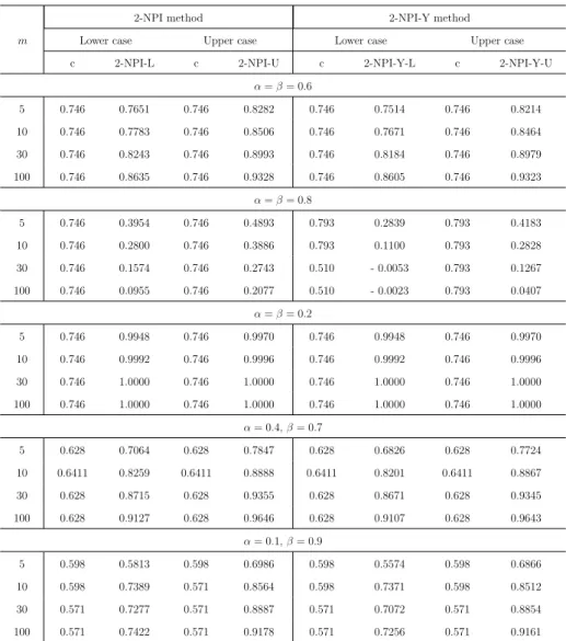
m

2-NPI method 2-NPI-Y method Lower case Upper case Lower case Upper case c 2-NPI-L c 2-NPI-U c 2-NPI-Y-L c 2-NPI-Y-U

α=β= 0.6 5 0.746 0.7651 0.746 0.8282 0.746 0.7514 0.746 0.8214 10 0.746 0.7783 0.746 0.8506 0.746 0.7671 0.746 0.8464 30 0.746 0.8243 0.746 0.8993 0.746 0.8184 0.746 0.8979 100 0.746 0.8635 0.746 0.9328 0.746 0.8605 0.746 0.9323 α=β= 0.8 5 0.746 0.3954 0.746 0.4893 0.793 0.2839 0.793 0.4183 10 0.746 0.2800 0.746 0.3886 0.793 0.1100 0.793 0.2828 30 0.746 0.1574 0.746 0.2743 0.510 - 0.0053 0.793 0.1267 100 0.746 0.0955 0.746 0.2077 0.510 - 0.0023 0.793 0.0407 α=β= 0.2 5 0.746 0.9948 0.746 0.9970 0.746 0.9948 0.746 0.9970 10 0.746 0.9992 0.746 0.9996 0.746 0.9992 0.746 0.9996 30 0.746 1.0000 0.746 1.0000 0.746 1.0000 0.746 1.0000 100 0.746 1.0000 0.746 1.0000 0.746 1.0000 0.746 1.0000 α= 0.4,β= 0.7 5 0.628 0.7064 0.628 0.7847 0.628 0.6826 0.628 0.7724 10 0.6411 0.8259 0.6411 0.8888 0.6411 0.8201 0.6411 0.8867 30 0.628 0.8715 0.628 0.9355 0.628 0.8671 0.628 0.9345 100 0.628 0.9127 0.628 0.9646 0.628 0.9107 0.628 0.9643 α= 0.1,β= 0.9 5 0.598 0.5813 0.598 0.6986 0.598 0.5574 0.598 0.6866 10 0.598 0.7389 0.571 0.8564 0.598 0.7371 0.598 0.8512 30 0.571 0.7277 0.571 0.8887 0.571 0.7072 0.571 0.8854 100 0.571 0.7422 0.571 0.9178 0.571 0.7256 0.571 0.9161

Table 2.3: Optimal threshold c and corresponding value of NPI-L, 2-NPI-U, 2-NPI-Y-L, 2-NPI-Y-U, using the 2-NPI and 2-NPI-Y

methods and mx=my =m

Table 2.3 provides the optimal threshold value cobtained from the two NPI-based methods along with their corresponding lower and upper probabilities, for mx =my. We

(30)

0.6, both NPI-based methods give the same optimal threshold value, c∈(0.746,0.769), regardless of the value of m.

On increasing the values ofαand β (α=β = 0.8), the 2-NPI method gives the same optimal threshold value as α =β = 0.6 scenario, whereas for the 2-NPI-Y the optimal threshold is c ∈ (0.793,0.800), regardless of the value of m; except for the 2-NPI-Y-L, the optimal threshold is c ∈ (0.510,0.543) for m = 30,100. In this scenario the values of lower and upper probabilities for both the methods are very low as they struggle to meet the required criterion. It is noticed that the 2-NPI-Y-L can be less than zero, this is because the lower probability of the number of correctly classified future individuals from groups X and Y in Equation (2.10) are very low. When the required criteria are easy to achieve (α=β = 0.2), both the methods perform well as these corresponding lower and upper probabilities are very high and both the 2-NPI and 2-NPI-Y methods provide the same optimal threshold, which is c∈(0.746,0.769), regardless of the value of m.

For α = 0.4,β = 0.7, as this scenario requests to put more emphasis on the number of correctly classified future individuals from group Y than that of group X, it is clear that the optimal threshold cfor both methods decreases in order to achieve the desired criteria in comparison to the α=β scenario. In addition, the optimal threshold changes with different values of m, for example, for m = 10 the optimal threshold for both the NPI-based lower and upper probabilities is c∈(0.6411,0.642), whereas form= 5,30,100, the optimal threshold is c ∈ (0.628,629). For the extreme case with α = 0.1, β = 0.9 where the desired criterion strongly emphasises the number of future observations from group Y, the optimal threshold value c decreases to achieve the required criterion in comparison to the α=β scenario, which isc∈(0.598,0.602) for m= 5,10 for both the methods, except for m= 10, the optimal threshold for the 2-NPI-U is c∈(0.571,0.572), and for larger values of m, m = 30,100, the optimal threshold for both the methods is c∈(0.571,0.572).

(31)

2.5. Examples 23

mx my

α=β= 0.6 10 6 0.746 0.6971 0.746 0.7723 0.746 0.6799 0.746 0.7651 30 40 0.746 0.8315 0.746 0.9070 0.746 0.8259 0.746 0.9057 60 100 0.746 0.8592 0.746 0.9306 0.746 0.8557 0.746 0.9299 α=β= 0.8 10 6 0.746 0.2955 0.746 0.3962 0.793 0.1457 0.793 0.3066 30 40 0.746 0.1404 0.746 0.2550 0.510 -0.0042 0.793 0.0964 60 100 0.746 0.0981 0.746 0.2087 0.510 -0.0023 0.793 0.0371 α= 0.4,β= 0.7 10 6 0.628 0.6656 0.628 0.7585 0.628 0.6387 0.628 0.7458 30 40 0.628 0.8774 0.628 0.9398 0.628 0.8734 0.628 0.9389 60 100 0.628 0.9056 0.628 0.9597 0.628 0.9033 0.628 0.9593

Table 2.4: Optimal threshold c and corresponding value of NPI-L, 2-NPI-U, 2-NPI-Y-L, 2-NPI-Y-U, using the 2-NPI and 2-NPI-Y methods and mx6=my

Table 2.4 provides the optimal threshold value cobtained from the two NPI-based methods along with their corresponding lower and upper probabilities for mx 6= my.

Comparing this table with Table 2.4, with respect to the optimal threshold, the optimal thresholds for α = β = 0.6 and α = β = 0.8 are found to be the same, whereas for α = 0.4, β = 0.7, the optimal threshold is c∈ (0.628,0.629), regardless of the values of mx and my. Again, in this table, the 2-NPI-Y-L can be less than zero since the lower

probability of the number of correctly classified future individuals from groups X and Y in Equation (2.10) are very low.

Over all, it is clear from the results in this example that the optimal threshold can change depending on the values of α andβ and also on the value of m. The maximum values of the empirical Youden index (EYI) and maximum area (EMA) are equal to 0.5696 and 0.6087, respectively, and the optimal threshold for both methods is c∈(0.793,0.800) As Example 2.1 involved a data set with the data from the two groups quite a bit overlapping, we now consider a small example with more separate data for the two groups.

Example 2.2. Consider an artificial data set for groupsX andY withnx =ny = 10,

con-sisting of the ranks,X ={1,2,3,4,6,7,8,9,10,12}andY ={5,11,13,14,15,16,17,18,19, 20}.

(32)

m

α=β= 0.6 5 10 0.8521 10 0.9565 10 0.8462 10 0.9560 10 10 0.8641 10 0.9678 10 0.8591 10 0.9675 25 10 0.8843 10 0.9787 10 0.8807 10 0.9786 100 10 0.9019 10 0.9856 10 0.8993 10 0.9855 α=β= 0.8 5 10 0.5749 10 0.8186 10 0.5165 10 0.8095 10 10 0.5027 10 0.8006 10 0.4180 10 0.7895 25 10 0.4424 10 0.7937 10 0.3303 10 0.7818 100 10 0.4092 10 0.7949 10 0.2715 10 0.7831

Table 2.5: Optimal threshold c and corresponding value of NPI-L, 2-NPI-U, 2-NPI-Y-L, 2-NPI-Y-U, using the 2-NPI and 2-NPI-Y

methods and mx=my =m

Table 2.5 provides the optimal threshold valuescobtained from the 2-NPI and 2-NPI-Y methods along with their corresponding lower and upper probabilities, formx =my =m.

We have considered two different scenarios of α and β. Forα =β = 0.6, both NPI-based methods give the same optimal threshold, c∈(10,11), regardless of the value of m, with high values of the lower and upper probabilities since the data from each group are less overlapping. The same results hold for α=β = 0.8, but with lower values of the lower and upper probabilities. The maximum values of the empirical Youden index (EYI) and maximum area (EMA) are equal to 0.8000 and 0.8100, respectively, and the optimal threshold value for both the methods is c∈ (10,11). It is clear that both the methods provide high values of the probability.

2.6 Simulation

In order to study the performance of the methods presented in this chapter, a simulation study was conducted for the two-group scenarios. We have considered two main cases, in which the data are simulated from the following normal distributions:

(33)

2.6. Simulation 25

Case A: X ∼N(0,22_{) and} _Y _∼_N₍₁_,₂2_).

Case B: X ∼N(0,12_{) and} _Y _∼_N₍₁_,₁2_).

Due to the larger variance in Case A, the groups in that case overlap more than in Case B, with the means in case A being one standard deviation apart while they are 0.5 standard deviation apart in case B. We simulatenx andny from the two normal distributions. Then,

thenx andny simulated data observations will be used to find the optimal thresholdsc

according to these methods and for specific values of (α, β) when applicable, where the threshold values are set to the midpoint in the partition of_Rused by the data. After that, we simulatemxandmy future observations from the same underlying normal distributions

as the nx and ny simulated data observations to see how the methods perform.

The mx and my simulated future observations are compared with the optimal

thresholds to obtain the number of correctly classified observations per group. We have studied the predictive performance of all methods in terms of the number of correctly classified future observations that are achieved using the desired criterion, that is when the number of correctly classified future observations from group X and Y exceedαmx

and βmy, respectively. Let us denote by ‘+’ when the desired criterion is achieved and

‘−’ otherwise. Throughout this simulation we assume that nx =ny and mx =my, and

jx, jy ∈ {0,1, . . . , m}.

We have run the simulation for n= 10 and m= 5,30, and we have chosen different values ofαandβ. Obviously the empirical Youden index and the maximum area methods do not depend on the values of α and β in terms of selecting the optimal thresholds. However for the comparison of predictive performance we have considered the same desired criterion of the number of future observations that are correctly classified from groups X and Y being at least αmx and βmy, respectively. The results in this section

are based on 10,000 simulations per case per method.

To search for the optimal threshold c, rather than searching for the value c that maximises the probability within each of the nx+ny + 1 intervals created by the data

observations, which could be computationally demanding especially in the simulation, we just consider the intervals as discussed in Section 2.2, that is we only consider the

(34)

threshold c to be in intervals between an observation from group X to the left and an observation from groupY to the right, and we also consider the first and the last intervals.

The predictive performance results for Case A are given in Tables 2.6 and 2.7 for m= 5 andm= 30, respectively, and in Tables 2.8 and 2.9 for Case B. We have studied the performance in two shapes forα=β with values 0.2,0.6 and 0.8, and forα= 0.4, β = 0.7, for the NPI-based methods (2-NPI and 2-NPI-Y) and the empirical estimates of the Youden index and maximum area methods (2-EYI and 2-EMA).

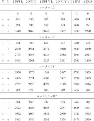
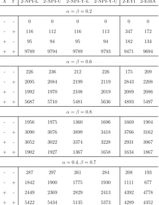
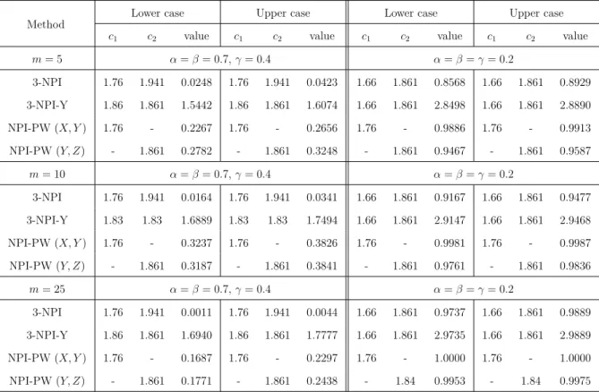
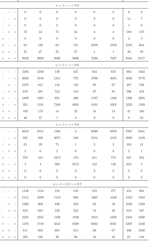
Consider Table 2.7, for example, where ‘+ +’ indicates that the desired criteria are achieved for both groups while ‘− −’ indicates that the desired criteria for both groups are not achieved. For example, for 2-NPI-Y-U and α=β = 0.2, the desired criteria have been achieved for both groups in 9886 out of 10,000 simulations, that is, at least 6 future observations (αm= 0.2×30 andβm = 0.2×30) are correctly classified from each of the disease and non-disease groups. On the other hand, in 62 out of 10,000 simulations, the desired criterion is achieved (6 or more out of 30 are correctly classified) for groupX, but the desired criterion is not achieved for group Y.

From Tables 2.6-2.9, the 2-NPI method outperforms all the other methods and for all the settings that have been considered for achieving the desired criterion for both

groups. While for small values of α and β, it appears that the 2-NPI and 2-NPI-Y

perform similarly, the 2-NPI-Y method performs poorly for larger values of αand β. One possible explanation is that the 2-NPI-Y method is based on the sum of the probabilities of correct classification rather than the product, which does not seem ideal if one tries to achieve higher proportions of those who are correctly classified. Yet for small values of α and β, as we have mentioned earlier, the 2-NPI-Y method performs equally well as the 2-NPI method.

Interestingly, the maximum area method (MA) is the closest in terms of performance to the 2-NPI method over all settings, yet the NPI method can be better, considering its predictive nature. It is not surprising that the maximum area method performs better than the Youden index method, as we have already discussed that summing the probabilities of correct classification may not be ideal when considering the prediction

(35)

performance.

In addition, we can see from these tables that for α=β = 0.6 and α=β = 0.8, all the methods perform better for small value of mthan for largerm, while forα=β = 0.2, all the methods perform better for large m than for small m; this is because of the randomness effect as discussed in Section 2.1. In general, we notice that all the methods, when they are not achieving the desired criterion on both groups X and Y, tend to reach the desired criterion for either group X or group Y. However, for larger values of α and β, the 2-NPI and 2-EMA methods mostly fail the desired criterion for each group. This result becomes clearer for larger m; for example, in Table 2.7, for α =β = 0.8 the 2-NPI and 2-EMA methods mostly fail the desired criterion for each group, whereas, the 2-NPI-Y method prefers to reach the desired criterion for either group X or group Y. It is obvious that if the values of α and β vary (α = 0.4, β = 0.7), the required criterion becomes either harder or easier to achieve, which depends on these values and the value of m. Clearly, all methods perform poorly with the increase of α and β as the criteria become harder to achieve, especially for α = β = 0.8. Finally, and not surprisingly, all methods perform much better in Case B than in Case A, as the groups in Case B are more separated than in Case A.

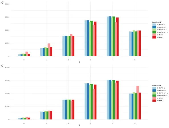
We summarise the number of correctly classified future observations in all simulations from groups X and Y using bar-plots as follows. Let the number of successfully classified future observations from group X with regards to the event of interest, which include α, be denoted by SX

jx and the number of successfully classified future observations from group Y with regards to the event of interest, which include β, be denoted by S_jY_y, where jx ∈ {0,1, . . . , mx}and jy ∈ {0,1, . . . , my}, respectively. Figures 2.1-2.4 show the

distributions of the numbers of future observations out of m in all 10,000 simulations, that are correctly classified for each group. For Case A, we can see that for larger values ofα =β, all methods struggle to meet the required criterion. Obviously, the performance for all methods becomes better for Case B since the groups have less overlap.

The results of this simulation show that the number of future observations considered and the values of α and β have an impact with regard to achieving the required criterion

(36)

of the number of future observations that are correctly classified from groups X and Y.

X Y 2-NPI-L 2-NPI-U 2-NPI-Y-L 2-NPI-Y-U 2-EYI 2-EMA

α=β= 0.2 - - 0 0 0 0 0 0 - + 301 293 301 294 890 424 + - 259 249 259 249 620 356 + + 9440 9458 9440 9457 8490 9220 α=β= 0.6 - - 793 795 664 747 540 741 - + 2869 2854 3372 3040 3844 3039 + - 2795 2787 2937 2882 3034 2911 + + 3543 3564 3027 3331 2582 3309 α=β= 0.8 - - 3556 3575 1684 2447 2734 3455 - + 2885 2874 4686 3902 3749 2999 + - 2797 2779 3325 3149 2962 2815 + + 762 772 305 502 555 731 α= 0.4, β= 0.7 - - 863 864 727 816 575 607 - + 2523 2727 2458 2887 1828 1031 + - 3072 2860 3833 2939 5121 5663 + + 3542 3549 2982 3358 2476 2699

Table 2.6: Simulation results (10,000 runs) for case A with n= 10 and

m = 5

X Y 2-NPI-L 2-NPI-U 2-NPI-Y-L 2-NPI-Y-U 2-EYI 2-EMA α=β= 0.2 - - 0 0 0 0 0 0 - + 52 50 54 52 752 185 + - 63 65 62 62 542 172 + + 9885 9885 9884 9886 8706 9643 α=β= 0.6 - - 867 890 586 797 488 751 - + 3943 3922 4753 4162 4905 4203 + - 3624 3595 3606 3617 3748 3696 + + 1566 1593 1055 1424 859 1350 α=β= 0.8 - - 7043 7186 1461 2701 5003 6746 - + 1495 1447 3327 4450 2899 1753 + - 1460 1365 5212 2848 2097 1499 + + 2 2 0 1 1 2 α= 0.4, β= 0.7 - - 274 277 210 266 154 181 - + 3105 3148 2718 3249 2630 1437 + - 3556 3450 4620 3539 5379 6236 + + 3065 3125 2452 2946 1837 2146

Table 2.7: Simulation results (10,000 runs) for case A with n= 10 and

(37)

Table 2.8: Simulation results (10,000 runs) for case B with n= 10 and

m = 5

Table 2.9: Simulation results (10,000 runs) for case B with n= 10 and

Nonparametric predictive inference for diagnostic test thresholds

Durham E-Theses

Nonparametric predictive inference for diagnostic test

thresholds

Nonparametric predictive inference

for diagnostic test thresholds

Manal H. Alabdulhadi

A thesis presented for the degree of

Doctor of Philosophy

Department of Mathematical Sciences

Durham University

United Kingdom

March 2018

for diagnostic test thresholds

Manal H. Alabdulhadi

Submitted for the degree of Doctor of Philosophy

March 2018

Declaration

Contents

Chapter 1

Introduction

1.1

Accuracy of diagnostic tests

1.2

Methods for selection of a threshold

1.3

Nonparametric Predictive Inference

1.3.1

A brief introduction

1.3.2

NPI for future order statistics

1.3.3

NPI for Bernoulli quantities

P

(

Y

≥

y

|

Y

=

s

) =

+

P

(

Y

< y

|

Y

=

s

) =

+

1.4

Outline of thesis

NPI for two-group diagnostic test

threshold

2.1

Introduction

2.2

NPI for two-group diagnostic test threshold

2.3

NPI method related to the two-group Youden

index

2.4

Searching for the optimal threshold

2.5

Examples

2.6

Simulation