Beta-boosted ensemble for big credit scoring data

(1)

SFB 649 Discussion Paper 2016-052

Beta-boosted ensemble

for big credit scoring data

Maciej Zieba *

Wolfgang K. Härdle*²

* Wroclaw University of Science and Technology, Republic of Poland *² Humboldt-Universität zu Berlin, Germany

This research was supported by the Deutsche

Forschungsgemeinschaft through the SFB 649 "Economic Risk". http://sfb649.wiwi.hu-berlin.de

ISSN 1860-5664

SFB 649, Humboldt-Universität zu Berlin Spandauer Straße 1, D-10178 Berlin

SFB

6

4

9 E

C

O

N

O

M

I

C

R

I

S

K

B

E

R

L

I

N

(2)

data

Maciej Zi˛eba, Wolfgang Karl Härdle

AbstractIn this work we present a novel ensemble model for a credit scoring prob-lem. The main idea of the approach is to incorporate separate beta binomial distri-butions for each of the classes to generate balanced datasets that are further used to construct base learners that constitute the final ensemble model. The sampling procedure is performed on two separate ranking lists, each for one class, where the ranking is based on prepotency of observing positive class. Two strategies are considered: one assumes mining easy examples and the second one forces good classification of hard cases. The proposed solutions are tested on two big datasets on credit scoring.

JEL classification:C53, Forecasting and Prediction Methods; Simulation

Key words: credit scoring, ensemble model, beta distribution, Beta boost, big data

Maciej Zi˛eba

Wroclaw University of Science and Technology, Wybrzeze Wyspianskiego 27, 50-370 Wroclaw, Poland, e-mail: [email protected]

Wolfgang Karl Härdle

Professor at Humboldt-Universität zu Berlin, Ladislaus von Bortkiewicz chair of statistics and Di-rector of C.A.S.E. - Center for Applied Statistics and Economics, Humboldt-Universität zu Berlin, Spandauer Straße 1, 10178 Berlin, Germany and School of Business, Singapore Management University, 50 Stamford Road, Singapore 178899. e-mail: [email protected]

Financial support from the Deutsche Forschungsgemeinschaft via CRC Economic Risk and IRTG 1792High Dimensional Non Stationary Time Series, Humboldt-Universität zu Berlin, is gratefully acknowledged.

(3)

1 Introduction

The problem of constructing a decision model to distinguish good and bad con-sumers can be defined as a dichotomous classification task, where the positive class (usually less numerous) represents "bad" applicants and the negative class stays be-hind "good" cases. Usually, instead of obtaining the binary classification result we aim at estimating the probability of credit repayment for each of the consumers. Basing on the probabilities the financial institution is capable to define the various profiles of the consumers. The common procedure for that kind of applications is to separate from training some group of labeled consumers and sort them according to the predictive probability using the trained model. The sorted group with the given labels is further used to distinguish the profiles. As a consequence, a higher patience is given to construct models that are characterized by good sorting capabilities than to the typical classifiers used for binary classification. Instead of maximizing the accuracy of predictionthe community working on the credit scoring models aims at achieve the highest value of AUC (area under ROC curve)criterion that stays behind sorting capabilities of the models.

Various machine learning algorithms were applied to solve credit scoring and fraud detection problems, such as: neural networks [13, 18, 22], Gaussian Processes [10], various extensions of SVMs (Support Vector Machines) [2, 3, 4, 7, 8, 9, 23] or comprehensible models based on neural structures [20] or SVMs [16].

Ensemble methods have also gained particular attention in the field of credit scoring. The general idea of this type of models is based on constructing many component models (so called base learners) that are joined together as one complex classifier. Usually, the base model is so-called weak learner that is characterized by poor individual performance, but strong learners are also used for particular en-semble models. Authors of [17] present very beneficial comparison of the standard ensemble procedures in application to credit scoring tasks. Some more up-to-date analysis of this kind of models for this particular application were presented in [1] and [24]. The most recent models make use of various types of base learners [11], joined two strategies of diversification on features and data levels [15], switching class labels [25], boosting neural networks [21] or using ensemble of cost-sensitive SVMs trained with active learning strategy [26]. Most recent studies studies show the great benefit of using Extreme Boosted Trees [27].

Here, we aim at constructing a novel boosting approach that works indepen-dently on selected base model and performs well on big credit scoring datasets. The key idea of this approach is to apply a strategy to sample examples for each of the boosting iterations to construct the base learners. We make use of particular Beta Binomial distributions that are applied to the sorted training data according to the prediction probabilities returned by current ensemble model. In this work we dis-tinguish two sampling strategies: the first strategy aims at sampling with the higher probability the examples that are already well located in the ranking. The other strat-egy is an example of so-calledhard examplesmining where the higher probabilities are given to the examples badly predicted and badly located in the ranking. Our approach was tested on the two benchmark datasets using two base models:

(4)

Logis-tic Regression and Decision Tree classifier. The results show that the first strategy works fine with the stable models like Logistic Regression, while the second strat-egy improves the quality of weak learners like Decision Trees.

The paper is organized as follows. In Section 2 we present theBetaBoost algo-rithm. In Section 3 we introduce some experimental studies investigating the perfor-mance of the approach. The paper is summarized with some conclusions presented in Section 4.

2 Method description

The main idea of the proposed approach is to create an ensemble model that makes use of re-sampling diversification technique in only to increase its sorting capa-bilities. To achieve the goal, each of the base learners is trained using re-sampled training data. The re-sampling procedure makes use of two particular beta binomial distributions (one for each class) that are used to generate indexes of examples that are going to be taken in the next boosting iteration. The crucial step in the training procedure is sorting the training data according to predictive capabilities of the so far created ensemble model. As a consequence, the examples with higher probabil-ity value have higher indexes and are going to be selected more often in training iterations. For the sampling sampling procedure we propose to useBeta Binomial distribution which is going to be characterized in the next subsection.

2.1 Beta Binomial distribution

The beta binomial distribution is selected because it is capable to assign high prob-abilities to particular regions of the sorted data according to predictive probability values of the training examples. Practically, it means that we are capable to concen-trate our model either on learning from difficult-to-distinguish credit consumers, or put the higher impact on learning from the easy-to-classify client applicants.

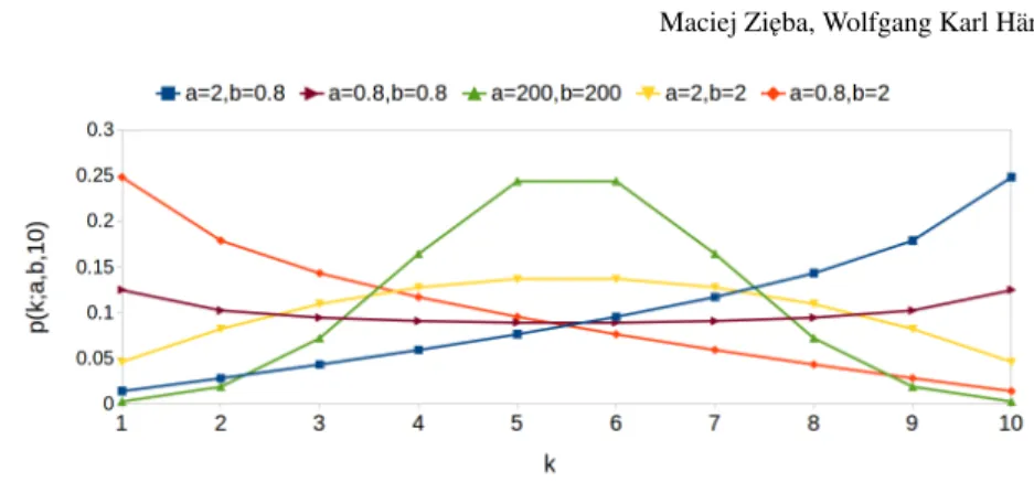
The flexibility of beta binomial distribution is controlled by three parameters:

• Shape parametersaandbthat are characteristic for beta distribution (a,b>0).

• ParameterNthat represents the number of trials characteristic for binomial dis-tribution (N∈N0).

The probability function for beta binomial distribution (BBin(a,b,N)) can be presented in the following form:

p(k;a,b,N) =

_N

k

_B₍_k₊_a_,_N₋_k₊_b₎

B(a,b) , (1)

whereB(a,b)is the beta function. The plots of the probability function for various values of the parametersaandbare presented in Figure 1.

(5)

Fig. 1: Probability mas function for beta binomial distribution considering various a,bvalues.

The presented distribution has the important property for the particular values of shape parametersaandb. In this application we are concentrating on particular families of beta binomial distributions:

• The subset of distributions, where a≤1, b≥1 and a6=b. If k1>k2, then p(k1;a,b,N)<p(k2;a,b,N).

• The subset of distributions, where a≥1, b≤1 and a6=b. If k1>k2, then p(k1;a,b,N)>p(k2;a,b,N).

The selection of the particular distributions is indicated by the strategies that are going to be applied to train the ensemble model. For the first strategy we aim at putting the higher impact on selecting better located examples in the rank-ing so for the rankrank-ing list for negative examples (sorted accordrank-ing to probabil-ity of observing positive class) we apply the family of distributions that satisfies p(k1;a,b,N)<p(k2;a,b,N), while for the ranking list for positive cases we use family of distribution that satisfies p(k1;a,b,N)>p(k2;a,b,N). As a consequence it is more probable to select the examples properly located on the both of the lists.

For the second strategy we make use of the first family of distributions for pos-itive ranking list and the second family for negative sorted samples. Contrary to previous strategy we aim at mining rather hard positive and negative examples and omitting well classified examples.

In the next section we present, how the beta binomial sampling is used in con-structing the boosted model.

2.2 Beta-boosted ensemble model

In this work we aim at constructing the ensemble classifier for binary classification y∈ {0,1}, composed ofT base models:

(6)

pT(y|x) = T

∑

t=0 ptp(y|x,t)y n 1−p(y|x,t)o (1−y) , (2)

wherexis vector of input features, p(y|x,t)representst-th base learner, and pt is

prior distribution over base learners.

For further work we assume that base learners are characterized by uniform dis-tribution, so we can present the ensemble model given by equation (2) in the fol-lowing form: pT(y=1|x) = 1 T+1 T

∑

t=0 p(y=1|x,t). (3) We are interested in obtaining probability value for a given positive class therefore we will further operate on probability for this class,p(y=1|x).

For the given predictorp(y=1|x)and the set of examplesXN={xn}Nn=1we can define the rank functionh(x,XN,p):

h(x,XN,p) = N

∑

n=1 Inp(y=1|x)>p(y=1|xn) o (4) The procedure for creating the ensemble classifier can be described by Algorithm 1. To create the classifier we make use of training data DN ={(xn,yn)}N_n=1, that contains N training examples: N1 positive and N0 negative instances. We aim at constructing the ensemble model given by the equation (3).

Algorithm 1:BetaBoost

Input:Training data:DN={(xn,yn)}Nn=1

Output:Ensemble model:pT(y=1|x)(see eq. (3))

Parameters:BBin0(·)parameters for negative class:a0,b0, BBin1(·)parameters for positive class:a1,b1, number of base learners:T+1.

1 SetX_N

1={xn:yn=1}andXN0={xn:yn=0}; 2 Train weak learnerp(y|x,0)with dataD_N; 3 fort←1toT do

4 Create ensemble predictorp_t−1(y=1|x) =_t+11 ∑tj=0p(y=1|x,j);

5 GenerateX˜(1)

N/2withsample(XN1,pt−1,a1,b1,N/2)(see Algorithm 2); 6 GenerateX˜(0)

N/2withsample(XN0,pt−1,a0,b0,N/2)(see Algorithm 2); 7 Create new training data ˜D_N= (X˜(1)

N/2,1)∪(X˜

(1)

N/2,0);

8 Train weak learnerp(y|x,k)with data ˜D_N; 9 end

To initialize the training procedure we distinguish positive and negative exam-ples denoting them by XN1 andXN2 respectively. We also initialize the

(7)

ensem-ble structure by training the first base learner p(y|x,0) using initial training set DN ={(xn,yn)}Nn=1. In the next step we perform constructing the committee ofT base classifiers in the training loop. Before creating the base learner we perform beta binomial sampling using separate distributions for each of the classes to obtainN/2 samples for each class. We use distributions for each of the classes,BBin0(a,b,N) to sample negatives andBBin1(a,b,N)to sample positives. We recommend to use particular families of distributions that was characterized in subsection 2.1.

Algorithm 2:Sampling procedure:sample(XN,p,a,b,Nout)

Input:Predictorp(y=1|x), the set of examplesXN={xn}N_n=1, number of output samplesNout.

Output:Set of data samples ˜XNout={xn}N_n=1out

Parameters:BBin(·)parameters:a,b.

1 X˜₀←/0;

2 forn←1toN_outdo

3 Samplek∼BBin(a,b,N−1);

4 X˜_n←X˜_n−1∪ {x∈XN:h(x,XN,p) =k},h(x,XN,p)is given by eq. (4);

5 end

The procedure of sampling the data makes use of the currently created ensem-ble model pt−1(y=1|x)to determine the ranking position of the examplexin the given setXN using ranking function h(x,XN,p) given by equation (4). The

sam-pling procedure is performed independently for each of the classes and is described by Algorithm 2. First, we sample the integerkfromBBin(a,b,N−1)distribution. Second, we identify the sample that has ranking value equal to the sampledkvalue and include it into the set of output samples ˜Xn. The sampling procedure is repeated

Nout times to obtain the output set of examples, ˜XNout. The procedure is equivalent

to sorting the given data according to the given predictions and then sampling their position with beta binomial distribution.

The sampling procedure is performed separately for the sets of positive and neg-ative examplesXN1,XN0 and, as a consequence, the new setsX˜

(1)

N/2andX˜

(0)

N/2are

created and each of them containsN/2 sampled examples. The two set are then la-beled and concatenated to the new training data ˜DN that is further used to train the

k-th base learner p(y|x,k). The procedure is repeatedT times to obtain ensemble model composed ofT+1 base learners.

2.3 Toy example

Consider the toy example in which we have set of 15 examples, 5 from positive class and 10 from negative class. Assume, that we have the committee of the models that sorted the training examples according to the predictive probabilityp(y=1|x)(see Figure 2a). Further, we assign individual ranking position for each of the considered

(8)

p0(y=1|x)

0 1

(a) Sorted data points according to the predictive distribution.

p0(y=1|x)

0 1

0 1 2 0 3 4 5 1 6 7 8 2 9 3 4

(b) Sorted data points with individual rankings for each class.

Fig. 2: The set of data examples sorted according top0(y=1|x). Red circles repre-sent negative examples, and green circles stand behind positive cases.

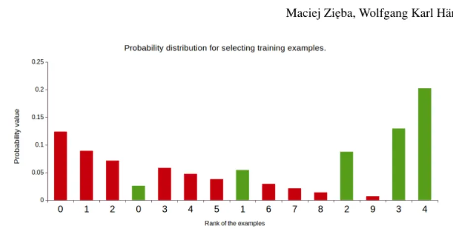
classes (see Figure 2b). Next, we assume individual Beta binomial distribution for each of the classes:

• BBin0(0.8,2,9)for negative examples.

• BBin1(2,0.8,4)for positive examples.

The selected distributions are consistent with the first strategy described in sub-section 2.1, where we aim at mining easy examples from both classes. We take arbitrary values of the parameters (a0=0.8,b=2,a=2,b=0.8) just to illustrate the proposed algorithm. Considering real applications, the selection of theaandb is crucial for the training procedure. If the both values are close to 0 the distribution approaches uniform distribution, while for largeaand smallbexamples with high positions are going to be selected multiple times. To select proper parameters for the distributions model selection procedure should be applied.

If we assume equal prior probabilities for selecting examples from minority and majority class, the sampling distribution for the next boosting iteration is presented in Figure 2.

If perform sampling with replacement from the given distribution we can obtain the set of examples that should be taken into next boosting iteration that is presented in Figure 4a. After learning the second base learner p(y=1|x,1)and adding it to the ensemble modelp1(y=1|x) = p(y=1

|x,0)+p(y=1|x,1)

2 we obtain the better sorting of the data (see Figure 4b).

If we consider the AUC criterion (area under ROC curve) that represents the quality of the sorting capabilities for the binary classification models it increases from 0.76 to 0.92.

The idea that stays behind the proposed procedure is a proper selection of the sampling distributions the satisfy the conditions that are described in subsection 2.1. In this variant we take the distribution for sampling positive examples that sat-isfies:a1≥1, b1≤1 and for sampling negative instances we use the distribution with parameters:a0≤1,b0≥1. Practically it means, that we aim at putting the higher impact on the examples that are characterized by higher predictive

(9)

probabil-Fig. 3: Sampling distribution for examples presented in Figure 2 -BBin0(0.8,2,9) for negative andBBin1(2,0.8,4)for positive examples.

p0(y=1|x) 0 ₁ 0 1 2 0 3 4 5 1 6 7 8 2 9 3 4 0 1 1 4 4 4

(a) The data sampled from distribution presented in Figure 3 (Grey circle stays behind unselected sample).

p1(y=1|x)

0 1

0 1 2 5 3 4 0 6 7 8 9 1 2 3 4

(b) The new order based on the classification of the ensemble modelp1(y= 1|x) =p(y=1|x,0)+₂p(y=1|x,1).

Fig. 4: The illustrative example presenting the capabilities of the joined ensemble model, after training the second base learner on the sampled data.

ities (for positive examples), or lower probability values (for negative examples). Our philosophy for this particular case is to put the higher impact on distinguishing the examples located away from each other in the global ranking determined by the predictions comparing to examples located in the weighted middle of the ranking list. As a consequence, we are sacrificing some portion of difficult to distinguish examples by putting them to unsure region, but we avoid observing them in low or high ranking positions. So the model has some capability to prevent overfitting that can be caused by discursive (or even noise) examples in training data. We also aim at dealing with imbalanced data phenomenon by sampling equal number of positive and negative examples.

(10)

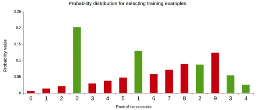
Fig. 5: Sampling distribution for examples presented in Figure 2 -BBin0(2,0.8,9) for negative andBBin1(0.8,2,4)for positive examples.

• BBin0(2,0.8,9)for negative examples.

• BBin1(0.8,2,4)for positive examples.

In this case, the sampling distribution for the next boosting iteration is presented in Figure 5. Following this strategy we aim at correct classification of the improperly ranked examples, assuming that they are rather hard examples that we manage to classify by the ensemble model.

The two presented strategies aim at different cases. In the first case we trust our base model, but we do not trust to our data assuming that there are some portion of the examples that are impossible to be distinguished. Therefore, we are leaving some portion of examples in controversial area on the ranking, cleaning low and high ranking regions with improperly located samples. For the second strategy, we use rather untrusted weak learner as a base model, but we aim at create the com-plex model that will properly classify hard instances if their impact is going to be decreased.

2.4 Relation to existing solutions

The presented work is inspired by existingRankBoost[5] (for which the equiva-lence to well knownAdaBoostwas described in [19]) method and couple of other approaches. In contrast to theRankBoostwe define two separate ranking functions for positive and negative examples. First of all, theRankboostapproach is very sen-sitive to the noisy examples located in training data.BetaBoostmodel presented in this paper deals well with insecure and noisy data because the distribution is not updated in iterations and does not depend on global ranking. Moreover, it is also more beneficial to use more flexible sampling distribution that is characterized by two parameters (aandb) contrary to the specific exponential-based distribution used

(11)

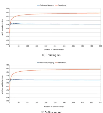
(a) Training set.

(b) Validation set.

Fig. 6: A comparison analysis ofBetaBoost(a0=0.8,b0=2,a1=2 andb1=0.8) andBalanced Baggingfor the growing number of base learners onGMSCdataset. We considerLogistic Regressionas base learner.AUCis taken as quality criterion.

in typical boosting approaches. The proposed solution is also inheriting self-paced philosophy [12] if the strategy with the increasing probabilities for positive and with decreasing probabilities for negative examples is applied.

As the procedure is independent on global ranking it is crucial to apply proper model selection procedure that will fit proper sampling curves for each of the classes.

3 Experiments

We are going to evaluate our approach on two large datasets from credit scoring domain that are available inKagglerepository:

(12)

(a) Training set.

(b) Validation set.

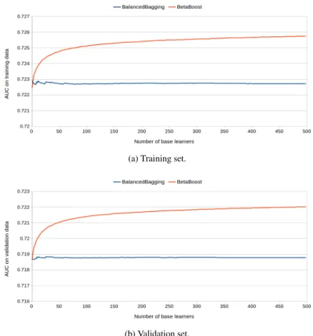
Fig. 7: A comparison analysis ofBetaBoost(a0=0.8,b0=2,a1=2 andb1=0.8) andBalanced Baggingfor the growing number of base learners onLCLDdataset. We considerLogistic Regressionas base learner.AUCis taken as quality criterion.

• Give me Some Credit[6].

• Lending Club Loan Data[14].

Give me Some Credit (GMSC)dataset is composed of 150000 examples, 10026 positive and 139974 negative elements. Each of the credit consumers is represented by the vector of 10 numeric features. Each of the attributes were normalized before using it for training.

Lending Club Loan Data(LCLD) dataset is composed of 887379 examples, 67429 positive and 819955 negative cases. Each of the examples were described by 12 features, where 6 of them were numeric, and the remaining 6 were nominal. On the preprocessing stage we have normalized the numeric features and binarized nominal attributes.

(13)

(a) Training set.

(b) Validation set.

Fig. 8: A comparison analysis of BetaBoost (a0=1.5, b0=0.8, a1=0.8 and b1=1.5) andBalanced Baggingfor the growing number of base learners onGMSC dataset. We consider Logistic Regressionas base learner.AUC is taken as quality criterion.

We divide each of the initial datasets to: training set (80% examples) and test set (20% examples). From training set we separate 10% instances for validation to monitor the training progress and select the best set of base learners.

For the evaluation we useAUC (area under ROC curve)criterion, which is often for evaluating credit scoring models and measures well the sorting capabilities of learners. For each of the scenarios we apply model selection of the sampling param-eters (a1,b1,a0,b0) from the set of candidates and select the parameters with the highestAUCobtained on the validation set.

We consider the two scenarios that were described in this work. In the first of the scenarios we aim at putting higher weights to the "secure" examples, assuming that controversial examples are hard to classify.

(14)

(a) Training set.

(b) Validation set.

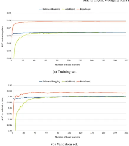
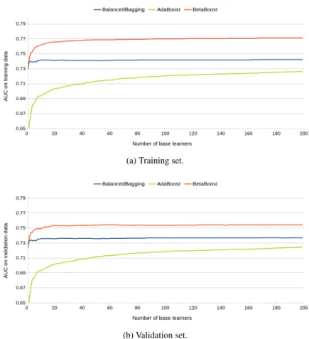
Fig. 9: A comparison analysis ofBetaBoost(a0=1.2,b0=0.8,a1=0.8 andb1= 1.2),Balanced BaggingandAdaBoostfor the growing number of base learners on LCLDdataset. We considerDecision Treeas base learner.AUCis taken as quality criterion.

p(y=1|x,k) =σ(wT_kx) = 1

1−exp{−wT

kx}

(5) At first we analyze the training capabilities of theBetaBoostmodel trained using the following beta parameters:a0=0.8,b0=2,a1=2 andb1=0.8. We compare the proposed approach with so called Balanced Bagging that performs sampling with replacement from uniform distribution to obtainN/2 samples from each class. The results of the comparison are presented in Figure 6 and 7.

It can be observed, thatLogistic Regressionis a very stable model characterized by small variance of the performance. Practically, it means that small changes in data caused by uniform sampling does not affect the overall performance of the

(15)

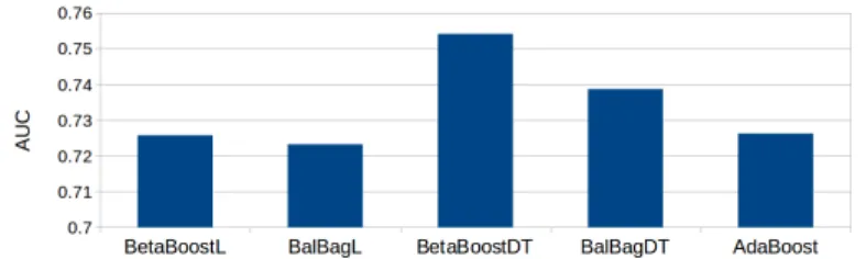
Fig. 10: Final results for considered models -GMSCdataset (test data)

Fig. 11: Final results for considered models -LCLDdataset (test data)

model. If we apply sampling for the procedure characteristic forBetaBoostmodel we would obtain the improvement ofAUCmeasure as it is observed in Figures 6 and 7. As a consequence of increasing probabilities for positive examples (a1>1 and b1<1) and decreasing probabilities for negative cases (a0<1 andb0>1) we aim at good quality prediction of the positive examples that are located on higher ranking positions and negative examples that are located on low positions. To obtain the goal we sacrifice the "difficult" examples that are suspected to be "noisy" instances, that are located in the discussion area. As a consequence, the improvement ofAUC is observed for both of the considered datasets.

As a second base model we propose to useDecision Trees. As a fact that this model is recognized as so calledweak learner, we propose the following sampling parameters to train theBetaBoostmodels:

• a0=1.5,b0=0.8,a1=0.8 andb1=1.5 forGMSCdataset,

• a0=1.2,b0=0.8,a1=0.8 andb1=1.2 forLCLDdataset.

The results are presented in Figures 7 and 8. We can see that sampling with replacement using the second strategy (a0≥1,b0≤1 anda1≤1,b1≥1) makes significant improvement ofAUCcriterion comparing toBetaBooststrategy, that also uses decision tree as a base learner. We also consider in the analysis theAdaBoost classifier that learns the component base model using the similar strategy that in-creases the impact of "hard examples", decreasing the significance of well predicted instances. TheAdaBoost model needs more iterations to achieve acceptableAUC level because both datasets are spoiled by imbalanced data phenomenon. The perfor-mance ofAdaBoostis similar toBetaBoostonGMSCdataset, but onLCLDdataset

(16)

it gives significantly worse results. We also present the results on validation data to show that overfitting problem is not observed for the considered models.

We presented the final results obtained by the considered models in Figures 10 (GMSCdataset) and 11LCLDdataset. The considered models are as follows:

• BetaBoostL.BetaBoostwithLogistic Regressionas base learner trained with the first strategy (a0≤1,b0≥1 anda1≥1,b1≤1).

• BalBagL.Balanced BaggingwithLogistic Regressionas a base learner.

• BetaBoostDT.BetaBoostwith a decision tree as a base learner trained with the second strategy (a0≥1,b0≤1 anda1≤1,b1≥1).

• BalBagDT.Balanced Baggingwith a decision tree as a base learner.

• AdaBoost.AdaBoostclassifier with a decision tree as a base learner.

It can be observed, that theBetaBoostwith decision tree as a base learner train with the second strategy performed better then the reference approaches considered in the experiments. On (GMSCdataset) we observed only slight increase in quality of BetaBoost comparing to Balanced Bagging from 0.8652 to 0.8673. However, we operate onbig data, so the slight improvements in quality criterion may have great impact on financial benefit. The improvement observed on theLCLDdataset is indisputable.

4 Conclusions and Future Works

In this work we propose alternative ensemble based strategy, that makes use of beta binomial sampling to create the base models. Two strategies can be distinguished while taking the sampling distribution. In the first strategy we aim at putting higher impact on "easy examples", we bestow trust the base model and do not trust in data quality. In the second strategy we take rather weak and unstable base model and we put the higher impact on training "hard examples".

Contrary to existing approaches likeAdaBoost, we update the sampling distribu-tion basing only on individual ranking for each of the classes. As a consequence, the impact of noisy examples in training data is not high.

The crucial step for the proposed theBetaBoostmodel is to find proper parame-ters for sampling distributions. It can be performed by grid search, but this approach is ineffective for large data sets. In the future works we plan to propose the smart model selection approach to solve that issue. Additionally, we are going to per-form more per-formal discussion of the properties of the proposed model. Moreover, the weighted variant of ensemble model is going to be proposed.

(17)

References

1. Abellán J, Mantas CJ (2014) Improving experimental studies about ensembles of classifiers for bankruptcy prediction and credit scoring. Expert Systems with Applications 41(8):3825–3830

2. Bellotti T, Crook J (2009) Support Vector Machines for credit scoring and dis-covery of significant features. Expert Systems with Applications 36(2):3302– 3308

3. Chen S, Härdle WK, Jeong K (2010) Forecasting volatility with Support Vector Machine-based GARCH model. Journal of Forecasting 29(4):406–433 4. Chen S, Härdle W, Moro R (2011) Modeling default risk with Support Vector

Machines. Quantitative Finance 11(1):135–154

5. Freund Y, Iyer R, Schapire RE, Singer Y (2003) An efficient boosting algorithm for combining preferences. Journal of machine learning research 4(Nov):933– 969

6. Give me Some Credit (2011) Give me Some Credit. https://www.kaggle.com/c/GiveMeSomeCredit

7. Härdle W, Lee YJ, Schäfer D, Yeh YR (2009) Variable selection and oversam-pling in the use of smooth Support Vector Machines for predicting the default risk of companies. Journal of Forecasting 28(6):512–534

8. Härdle WK, Prastyo DD, Hafner C (2012) Support Vector Machines with Evo-lutionary Feature Selection for Default Prediction. Handbook of Applied Non-parametric and Semi-Non-parametric Econometrics and Statistics pp 346–373 9. Harris T (2015) Credit scoring using the clustered Support Vector Machine.

Expert Systems with Applications 42(2):741–750

10. Huang SC (2011) Using Gaussian process based kernel classifiers for credit rating forecasting. Expert Systems with Applications 38(7):8607–8611 11. Koutanaei FN, Sajedi H, Khanbabaei M (2015) A hybrid data mining model of

feature selection algorithms and ensemble learning classifiers for credit scoring. Journal of Retailing and Consumer Services 27:11–23

12. Kumar MP, Packer B, Koller D (2010) Self-paced learning for latent variable models. In: Advances in Neural Information Processing Systems, pp 1189– 1197

13. Lee TS, Chiu CC, Lu CJ, Chen IF (2002) Credit scoring using the hybrid neural discriminant technique. Expert Systems with applications 23(3):245–254 14. Lending Club (2016) Lending Club Loan Data.

https://www.kaggle.com/wendykan/lending-club-loan-data

15. Marqués A, García V, Sánchez JS (2012) Two-level classifier ensembles for credit risk assessment. Expert Systems with Applications 39(12):10,916– 10,922

16. Martens D, Baesens B, Van Gestel T, Vanthienen J (2007) Comprehensible credit scoring models using rule extraction from Support Vector Machines. Eu-ropean journal of operational research 183(3):1466–1476

(18)

17. Nanni L, Lumini A (2009) An experimental comparison of ensemble of classi-fiers for bankruptcy prediction and credit scoring. Expert systems with applica-tions 36(2):3028–3033

18. Oreski S, Oreski D, Oreski G (2012) Hybrid system with genetic algorithm and artificial neural networks and its application to retail credit risk assessment. Expert systems with applications 39(16):12,605–12,617

19. Rudin C, Schapire RE (2009) Margin-based ranking and an equivalence be-tween AdaBoost and RankBoost. Journal of Machine Learning Research 10(Oct):2193–2232

20. Tomczak JM, Zi˛eba M (2015) Classification Restricted Boltzmann Machine for comprehensible credit scoring model. Expert Systems with Applications 42(4):1789–1796

21. Tsai CF, Wu JW (2008) Using neural network ensembles for bankruptcy pre-diction and credit scoring. Expert systems with applications 34(4):2639–2649 22. Zhao Z, Xu S, Kang BH, Kabir MMJ, Liu Y, Wasinger R (2015) Investigation

and improvement of multi-layer perceptron neural networks for credit scoring. Expert Systems with Applications 42(7):3508–3516

23. Zhou L, Lai KK, Yen J (2009) Credit scoring models with AUC maximization based on weighted SVM. International journal of information technology & decision making 8(04):677–696

24. Zhu Y, Xie C, Wang GJ, Yan XG (2016) Comparison of individual, ensemble and integrated ensemble machine learning methods to predict chinas sme credit risk in supply chain finance. Neural Computing and Applications pp 1–10 25. Zi˛eba M, ´Swi ˛atek J (2012) Ensemble classifier for solving credit scoring

prob-lems. In: Doctoral Conference on Computing, Electrical and Industrial Systems, Springer, pp 59–66

26. Zi˛eba M, Tomczak JM (2015) Boosted svm with active learning strategy for imbalanced data. Soft Computing 19(12):3357–3368

27. Zi˛eba M, Tomczak SK, Tomczak JM (2016) Ensemble boosted trees with syn-thetic features generation in application to bankruptcy prediction. Expert Sys-tems with Applications 58:93–101

(19)

SFB 649 Discussion Paper Series 2016

For a complete list of Discussion Papers published by the SFB 649,

please visit http://sfb649.wiwi.hu-berlin.de.

001 "Downside risk and stock returns: An empirical analysis of the long-run and short-run dynamics from the G-7 Countries" by Cathy Yi-Hsuan Chen, Thomas C. Chiang and Wolfgang Karl Härdle, January 2016.

002 "Uncertainty and Employment Dynamics in the Euro Area and the US" by Aleksei Netsunajev and Katharina Glass, January 2016.

003 "College Admissions with Entrance Exams: Centralized versus Decentralized" by Isa E. Hafalir, Rustamdjan Hakimov, Dorothea Kübler and Morimitsu Kurino, January 2016.

004 "Leveraged ETF options implied volatility paradox: a statistical study" by Wolfgang Karl Härdle, Sergey Nasekin and Zhiwu Hong, February 2016. 005 "The German Labor Market Miracle, 2003 -2015: An Assessment" by

Michael C. Burda, February 2016.

006 "What Derives the Bond Portfolio Value-at-Risk: Information Roles of Macroeconomic and Financial Stress Factors" by Anthony H. Tu and Cathy Yi-Hsuan Chen, February 2016.

007 "Budget-neutral fiscal rules targeting inflation differentials" by Maren Brede, February 2016.

008 "Measuring the benefit from reducing income inequality in terms of GDP" by Simon Voigts, February 2016.

009 "Solving DSGE Portfolio Choice Models with Asymmetric Countries" by Grzegorz R. Dlugoszek, February 2016.

010 "No Role for the Hartz Reforms? Demand and Supply Factors in the German Labor Market, 1993-2014" by Michael C. Burda and Stefanie Seele, February 2016.

011 "Cognitive Load Increases Risk Aversion" by Holger Gerhardt, Guido P. Biele, Hauke R. Heekeren, and Harald Uhlig, March 2016.

012 "Neighborhood Effects in Wind Farm Performance: An Econometric Approach" by Matthias Ritter, Simone Pieralli and Martin Odening, March 2016.

013 "The importance of time-varying parameters in new Keynesian models with zero lower bound" by Julien Albertini and Hong Lan, March 2016. 014 "Aggregate Employment, Job Polarization and Inequalities: A

Transatlantic Perspective" by Julien Albertini and Jean Olivier Hairault, March 2016.

015 "The Anchoring of Inflation Expectations in the Short and in the Long Run" by Dieter Nautz, Aleksei Netsunajev and Till Strohsal, March 2016. 016 "Irrational Exuberance and Herding in Financial Markets" by Christopher

Boortz, March 2016.

017 "Calculating Joint Confidence Bands for Impulse Response Functions using Highest Density Regions" by Helmut Lütkepohl, Anna Staszewska-Bystrova and Peter Winker, March 2016.

018 "Factorisable Sparse Tail Event Curves with Expectiles" by Wolfgang K. Härdle, Chen Huang and Shih-Kang Chao, March 2016.

019 "International dynamics of inflation expectations" by Aleksei Netšunajev and Lars Winkelmann, May 2016.

020 "Academic Ranking Scales in Economics: Prediction and Imdputation" by Alona Zharova, Andrija Mihoci and Wolfgang Karl Härdle, May 2016.

SFB 649, Spandauer Straße 1, D-10178 Berlin http://sfb649.wiwi.hu-berlin.de

Forschungsgemeinschaft through the SFB 649 "Economic Risk".

(20)

For a complete list of Discussion Papers published by the SFB 649,

please visit http://sfb649.wiwi.hu-berlin.de.

021 "CRIX or evaluating blockchain based currencies" by Simon Trimborn and Wolfgang Karl Härdle, May 2016.

022 "Towards a national indicator for urban green space provision and environmental inequalities in Germany: Method and findings" by Henry Wüstemann, Dennis Kalisch, June 2016.

023 "A Mortality Model for Multi-populations: A Semi-Parametric Approach" by Lei Fang, Wolfgang K. Härdle and Juhyun Park, June 2016.

024 "Simultaneous Inference for the Partially Linear Model with a Multivariate Unknown Function when the Covariates are Measured with Errors" by Kun Ho Kim, Shih-Kang Chao and Wolfgang K. Härdle, August 2016. 025 "Forecasting Limit Order Book Liquidity Supply-Demand Curves with

Functional AutoRegressive Dynamics" by Ying Chen, Wee Song Chua and Wolfgang K. Härdle, August 2016.

026 "VAT multipliers and pass-through dynamics" by Simon Voigts, August 2016.

027 "Can a Bonus Overcome Moral Hazard? An Experiment on Voluntary Payments, Competition, and Reputation in Markets for Expert Services" by Vera Angelova and Tobias Regner, August 2016.

028 "Relative Performance of Liability Rules: Experimental Evidence" by Vera Angelova, Giuseppe Attanasi, Yolande Hiriart, August 2016.

029 "What renders financial advisors less treacherous? On commissions and reciprocity" by Vera Angelova, August 2016.

030 "Do voluntary payments to advisors improve the quality of financial advice? An experimental sender-receiver game" by Vera Angelova and Tobias Regner, August 2016.

031 "A first econometric analysis of the CRIX family" by Shi Chen, Cathy Yi-Hsuan Chen, Wolfgang Karl Härdle, TM Lee and Bobby Ong, August 2016.

032 "Specification Testing in Nonparametric Instrumental Quantile Regression" by Christoph Breunig, August 2016.

033 "Functional Principal Component Analysis for Derivatives of Multivariate Curves" by Maria Grith, Wolfgang K. Härdle, Alois Kneip and Heiko Wagner, August 2016.

034 "Blooming Landscapes in the West? - German reunification and the price of land." by Raphael Schoettler and Nikolaus Wolf, September 2016. 035 "Time-Adaptive Probabilistic Forecasts of Electricity Spot Prices with

Application to Risk Management." by Brenda López Cabrera , Franziska Schulz, September 2016.

036 "Protecting Unsophisticated Applicants in School Choice through Information Disclosure" by Christian Basteck and Marco Mantovani, September 2016.

037 "Cognitive Ability and Games of School Choice" by Christian Basteck and Marco Mantovani, Oktober 2016.

038 "The Cross-Section of Crypto-Currencies as Financial Assets: An Overview" by Hermann Elendner, Simon Trimborn, Bobby Ong and Teik Ming Lee, Oktober 2016.

039 "Disinflation and the Phillips Curve: Israel 1986-2015" by Rafi Melnick and Till Strohsal, Oktober 2016.

(21)

SFB 649 Discussion Paper Series 2016

For a complete list of Discussion Papers published by the SFB 649,

please visit http://sfb649.wiwi.hu-berlin.de.

040 "Principal Component Analysis in an Asymmetric Norm" by Ngoc M. Tran, Petra Burdejová, Maria Osipenko and Wolfgang K. Härdle, October 2016. 041 "Forward Guidance under Disagreement - Evidence from the Fed's Dot

Projections" by Gunda-Alexandra Detmers, October 2016.

042 "The Impact of a Negative Labor Demand Shock on Fertility - Evidence from the Fall of the Berlin Wall" by Hannah Liepmann, October 2016. 043 "Implications of Shadow Bank Regulation for Monetary Policy at the Zero

Lower Bound" by Falk Mazelis, October 2016.

044 "Dynamic Contracting with Long-Term Consequences: Optimal CEO Compensation and Turnover" by Suvi Vasama, October 2016.

045 "Information Acquisition and Liquidity Dry-Ups" by Philipp Koenig and David Pothier, October 2016.

046 "Credit Rating Score Analysis" by Wolfgang Karl Härdle, Phoon Kok Fai and David Lee Kuo Chuen, November 2016.

047 "Time Varying Quantile Lasso" by Lenka Zbonakova, Wolfgang Karl Härdle, Phoon Kok Fai and Weining Wang, November 2016.

048 "Unraveling of Cooperation in Dynamic Collaboration" by Suvi Vasama, November 2016.

049 "Q3-D3-LSA" by Lukas Borke and Wolfgang K. Härdle, November 2016. 050 "Network Quantile Autoregression" by Xuening Zhu, Weining Wang,

Hangsheng Wang and Wolfgang Karl Härdle, November 2016.

051 "Dynamic Topic Modelling for Cryptocurrency Community Forums" by Marco Linton, Ernie Gin Swee Teo, Elisabeth Bommes, Cathy Yi-Hsuan Chen and Wolfgang Karl Härdle, November 2016.

052 "Beta-boosted ensemble for big credit scoring data" by Maciej Zieba and Wolfgang Karl Härdle, November 2016.