W
W
OR
O
RK
KI
IN
N
G
G
P
P
AP
A
PE
ER
R
NO
N
O
.
.
1
1
5
5
5
5
Informal Credit Markets, Judicial Costs
and Consumer
Credit: Evidence from Firm Level Data
Charles Grant and Mario Padula
February 2006
University of Naples Federico II University of Salerno Bocconi University, Milan CSEF - Centre for Studies in Economics and Finance–UNIVERSITY OF SALERNO
W
W
O
O
R
R
K
K
I
I
N
N
G
G
P
P
A
A
P
P
E
E
R
R
N
N
O
O
.
.
1
1
5
5
5
5
Informal Credit Markets, Judicial Costs
and Consumer
Credit: Evidence from Firm Level Data
Charles Grant
and Mario Padula
Abstract
How does the punishment for default affect repayment behavior? We use administrative data provided by the leading Italian lender of unsecured credit to the household sector to investigate the effect of two potentially important factors: judicial efficiency and the availability of informal credit from family and friends. By making economic assumptions we can place upper and lower bounds on these effects. We find that the availability of informal credit reduces repayment, while variation in court enforcement has no significant effect. Moreover, households with access to informal credit are more likely to borrow from our lender.
JEL Classification: D14, K42, O17
Keywords: Households Borrowing, Informal Credit Markets, Asymmetric Information
University of Reading. E-mail address: c.grant@reading.ac.uk.
University of Salerno and CSEF. E-mail address: mpadula@unisa.it. Mario Padula gratefully acknowledges financial support of the Finance and Consumption Chair in the European Community which enabled this project to be completed. Without involving them, we would like to thank for comments and suggestions at various stages of this project Alberto Bennardo, Giuseppe Bertola, Agar Brugiavini, John Duca, Burcu Duygan, Stefan Hochguertel, Winfried Koeninger, Tullio Jappelli, Theresa Osborne, and Frank Vella. We also would like to thank seminar participants at the University of Venice.
Contents
1. Introduction
2. Background literature 3. Data
4 The econometric model 5 Estimation
6. Results 7. Conclusions References
1
Introduction
Which households repay their debts and which borrowers default? Which factors affect repayment behavior, and how large are the effects? This paper addresses these questions and provides some evidence using data provided by the leading lender of unsecured credit to the Italian household sector. Credit markets in Italy are small by EU standards, but they grew quite rapidly over the past 20 years, as well documented by Casolaro, Gambacorta and Guiso (2005). The trend is similar for consumer credit (e.g. non-housing debt), which accounts for 8.1 percent of the GDP in 2003 and is largely unsecured. Theory predicts that incentives to repay depend crucially on how default is punished. We particularly focus on how the quality of judicial enforcement and the availability of informal credit markets affect households’ default on consumer credit contracts.
The incentives for individuals to default depends on the penalty incurred when not re-paying. If the debt is collateralized, and the debt is not repayed, then the property pledged as collateral is transferred to the creditor. The speed with which the asset is transferred depends, among others things, on how long it takes for the court to enforce the contract. Thus, enforcing debts more slowly makes it less costly for the borrower to fail to repay.
Using data on civil trials provided by the Italian Institute of Statistics (ISTAT), both Jappelli, Pagano and Bianco (2004) and Fabbri and Padula (2005) document the effect of judicial enforcement on credit to firms and households, respectively. Both studies exploit the large variation across Italy in judicial enforcement, and find significant effects on access to credit. Our approach is similar, with geographical variation in markets and institutions playing a major role in our analysis. However, in contrast to these papers, the focus is on the unsecured consumer credit market. Namely, we investigate the effect of judicial enforcement and of informal credit markets on borrowers’ repayment behavior.
Judicial enforcement affects the decision to lend through its effect on the value of the col-lateral. But for non-housing consumer credit, it is not obvious how the judicial enforcement affects the screening of loan applicants and thus borrower behavior. Given the small size of the loans, and that they are poorly collateralized, failure to repay usually only amounts to
being blacklisted and excluded from future borrowing in formal credit markets.1
The cost of exclusion will also depend on whether alternative sources of credit are avail-able. Households with access to credit from the informal sector are likely to view the deterrent effect of exclusion from the formal sector less seriously, and thus have lower incentives to repay debts incurred there. Among alternative credit providers, an important role is played by informal credit markets: around 3 percent of Italian households are indebted to family and friends. The use of these alternative credit providers is common throughout Italy but more prevalent in the South.
Other than affecting the borrowers’ outside option, there is another important way in which financial help from relatives or friends might affect repayment behavior. As empha-sized in a number of papers (see for instance Ghosh, Mookherjee and Ray, 2000), family networks have access to a better monitoring technology, and thus can lend to borrowers who would otherwise be unable to pay their debts in the formal sector. This can enable financially troubled borrowers to meet their payments on consumer credit contracts even when their assets would not allow them to do so and consequently makes default less likely.
The paper will thus investigate whether the availability of family and friends’ financial help makes borrower default more, or less likely. Furthermore, we investigate if the the effect of judicial enforcement on loan selection in the market for consumer credit differs from the previously studied market for housing debt.
We use a novel data-set drawn directly from the administrative records of the leading Italian lender of unsecured credit to the Italian household sector. The data provide detailed information on the characteristics of contracts, customers, repayment and, importantly, re-jected applications. Administrative data have a number of advantages. Since the data record the repayment history of applicants who were given credit, this allows us to observe default, which is a rare event in general household surveys. Even on the few occasions appropriate questions on default are included, this is likely to be underreported.2 A second advantage
1Even for installment credit, the resale value of the good would rarely cover the outstanding debt.
2For example, Fay, Hurst and White (2002) found that only around 250 US households reported filing for
bankruptcy in the 1996 wave of the PSID, around half the national filing rate. Moreover, and more seriously, only a small proportion of households in serious arrears result in a filing for bankruptcy.
is that administrative data records all the variables that affect the decision to lend, while survey data typically has only a subset of them. Finally, administrative data allows us to ob-serve both accepted and rejected applications, while survey data is rarely informative about rejected credit applications. This information is crucial if one wants to draw inference on household repayment behavior and account for the fact that that households granted credit, and those refused, are likely to be different.
The rest of the paper is organized as follows. Section 2 reviews some background liter-ature. The data are described in Section 3, while Section 4 deals with the selection issues involved in the use of a choice based sample. To investigate households’ repayment be-haviour, we must impute the probability that a household refused credit would default if the credit application had been accepted. This imputation can impose implausible economic assumptions, hence we provide upper and lower bounds on the estimated effect. Section 5 discusses parametric and semi-parametric estimation. The results are illustrated in Section 6, where we also discuss the role of asymmetric information in the consumer credit market, and argue that both moral hazard and adverse selection are present. Section 7 concludes.
2
Background literature
The early literature on the lender-borrower relationship, showed how asymmetric informa-tion could cause banks and other lenders to restrict access to credit (see, for instance, the pioneering work of Stiglitz and Weiss, 1981). In these models, default is exogenous but cred-itors can not tell a priori which agents will default and which will not, hence they offer the same contract to all borrowers. In contrast, Jaffee and Russell (1976) discussed how agents who do not bear the full consequences of their actions may indulge in riskier behaviour and hence be more likely to default on their debts. While this literature considered entrepreneurs, the insights are also relevant for consumption smoothing. In a more recent literature, Ke-hoe and Levine (1993) and Kocherlakota (1996) explicitly model the decision to default of infinitely lived consumers in a general equilibrium framework. Whether households default depends on how severely they are punished: agents compare the punishment for default with the gain from not repaying their debts. In these models, default is punished by autarky;
permanent exclusion from borrowing and saving in all future time periods. These studies show that credit constraints would arise endogenously since above some maximum level of debt, default is assured, and it is never rational for lenders to extend credit beyond this level. A key point in this literature is that incentives to default depend on the agents outside option. In empirical studies this is important since debtors can not be permanently excluded from credit markets. In the US, for example, bankruptcy can not be recorded in credit files for more than 10 years, and in practice, these households gain access to credit and to saving instruments much more quickly. Moreover, informal credit channels, such as friends and family, may be available to such households without interruption. Incentives to default will also depend on the cost of enforcing debts, in terms of both money and the time it takes for lenders to recover their debts. Making the enforcement of debt contracts more difficult makes lending less attractive for lenders. This paper will explicitly concentrate on studying these two issues.
While the relation between credit contracts and both the legal rules and their enforcement is widely studied (see for instance Fay, Hurst and White, 2002, Grant, 2003, and Fabbri and Padula, 2004), much less it has been said on the effect of non-market sources of credit. In a very different context, Banerjee and Newman (1998) show that these alternative credit sources can have important effects on development. They argue that in the formal sector, informational asymmetries can be large, while they are much smaller in the informal sector in which agents behaviour can be much more easily observed: friends and family are likely to know whether people they know closely are reliable and will repay their debts. In contrast, our paper provides empirical evidence (albeit on credit to consumers not producers) showing that in areas where informal credit is more common, households are less likely to repay their debts in the formal sector, everything else being equal.
While the theory is well understood, the evidence is scant. In their survey, Chiappori and Salani´e (2003) note that most of the empirical literature that assesses the theoretical impli-cations of asymmetric information does not investigate lending relationships. Moreover, few studies can distinguish between adverse selection and moral hazard. For example, Chiappori and Salani´e (2000) focus on the car insurance market and test the hypothesis that contracts with more comprehensive coverage are chosen by agents with a higher accident probability.
This robust correlation might equally arise because of adverse selection or moral hazard. The results are however negative, suggesting that the French car insurance market is not plagued by asymmetric information. In a later paper, Chiappori, Jullien, Salani´e and Salani´e (2005) provide similar evidence in a more general setting and argue that market power and risk aversion are responsible for the low correlation between coverage and accident probability.
Ausubel (1999) did investigate credit markets. His study explored the effect of a major US credit card company randomly offering different loan rates to different households. He found that borrowers had worse credit scores than non-borrowers and that households accepting inferior offers have worse credit scores than those with better offers but that all borrowers had worse credit scores than non-borrowers. However, since these characteristics are observable to the lender prior to the loan, they do not suggest adverse selection. To address this, Ausubel also found that after controlling for observable (to the lender) household characteristics, borrowers with worse offers are more likely to default. However, this paper does not explicitly investigate moral hazard, arguing that interest rate differences are too small for this to be important. Klonner and Rai (2005) also exploited exogenous differences in interest rates in India, where the government introduced interest rate ceiling. They find evidence that default rates are higher when interest rates were higher. They also note that social capital seems to mitigate adverse selection since default rates are higher in urban areas and in newly established branches, although they have no direct measure of social capital.3
Edelberg (2003), in contrast to these studies, disentangles adverse selection from moral hazard effects through a fully structural model and finds evidence for both. Like Ausubel (1999), Karlan and Zinman (2005) also exploit a randomized experiment. They focus on consumer credit market in South Africa, in which, again, households are randomly offered different loan rates. However, the innovation in their study is that after accepting the terms, some borrowers subsequently have their interest rate reduced. They argue this allows them to distinguish between adverse selection and moral hazard since adverse selection will affect acceptance at the initial offered loan rate, while moral hazard will affect repayment at the actual loan rate. They find evidence for both moral hazard and for adverse selection.
3That default rates are higher in urban areas is not fully consistent with the implications of Banerjee and
Our paper differs from these studies since we do not exploit differences in the interest rate: our lender offers standard debt contracts and the interest rate on their contracts does not differ across borrowers. Loan applications are either granted at the prevailing interest rate, or the request is turned down.4 This paper does not conduct an experiment either.
Rather, our study contains details on the applications for credit, whether they were granted, and whether the debt was repayed. We exploit variables that are not in the original data that is constructed by the lender (and hence do not enter their lending decision), and show that some of these variables affect repayment behaviour in the way that is predicted by theory: evidence which is consistent with moral hazard.
3
Data
We take data from three different sources, described in turn. For information on borrowing, we have a unique data set which consists of a random sample of households that are in the full administrative database of Findomestic Banca for 1995 - 1999. This data has been used in Alessie, Hochguertel and Weber (2005). Findomestic specializes in non-mortgage lending to the Italian household sector, much of it (61 percent in our sample) via instalment credit made available by the retailer at the point of sale. The bank also supplies revolving credit, in the form of credit cards. This type of contract amounts to 37 percent of our sample. Lastly, and rather less importantly, the bank offers personal loans, a market which it has entered more recently. Our lender is the market leader for these types of credit in Italy. In the data, the median debt is only 700 euros. Even though much of the debt is instalment credit, in practice the recovery value of the good which was purchased is small, hence Findomestic treats all the loans as unsecured, and does not attempt to repossess the good.5
In 1999, the last year for which we have data, our lender had three million customers in their credit records. From this they have provided a random sample approximately 120,000
4Edelberg (2003) showed that systematically offering different interest rates to different agents, conditional
on the borrowers observable characteristics (known as ‘risk-based pricing’ in the industry) is a comparatively recent phenomenon even in the US, and it is not currently practiced by Italian lenders.
clients, and since clients may have more than one contract, we have information on roughly 200,000 contracts. The lender has made all their customer information available to us, except the specific credit score for the customer. Their aim in collecting the data is to identify suitable consumers with which to build long-term relationships, such as middle-income families with steady jobs. The data records all applications that have been made by the household; whether credit was granted; and the repayment history of the household for each debt. The data also includes information about the household’s characteristics such as date of birth of the head and of the spouse, the profession of household members, the province and region of residence, seniority in the profession of the head and of the spouse, housing tenure, number of children, income and so on.
Compared to the Italian population as a whole, the households in our sample of credit applications are younger, have lower income, are more likely to be living in the South, and more likely to rent than is typical of the Italian population. For each client, we have informa-tion on all current and past contracts and all applicainforma-tions (including rejected applicainforma-tions), for each of the three types of loans that are granted. Moreover, some of the loans although authorized by the lender, were not activated by the customer.
For contracts that went into effect, we have information on the type of contract, the amount financed or the credit limit, the amount repaid or the credit actually extended, and the currently outstanding debt and repayment status of the borrower. The data for accepted applicants is a cross sectional snapshot of existing contracts, containing financial information on particular contracts (including the price of the good, the item financed, the amount of credit extended, and the currently outstanding debt), as well as some demographics and other background information on the customer, including the method of repayment. For revolving credit, it includes the outstanding amount and the credit limit. The data set also includes the bank’s evaluation of the customer and the contract in terms of the repayment behavior of the borrower. In about 15 percent of cases, applicants are refused credit. We have a random sample consisting of 5 percent of these rejected applications. This file records information similar to that which we have for accepted applicants. A few households have been rejected on some applications and have been successful in others.
reduced compared to survey data. Since the lender uses this information when screening the applicant and when assessing whether action needs to be taken against borrowers in arrears, it has strong incentives to ensure its accuracy. However, a disadvantage of using administrative data is that it contains less information about the characteristics of the household than most survey data, and any data on the household is self-reported by the applicant (who may have incentives to report falsely). Standard consistency checks on the data have been carried out as described in Alessie, Hochguertel and Weber (2005).
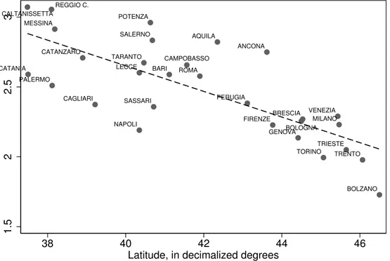
In order to construct our indicators of judicial efficiency and of borrowing from friends and relatives, we use two other data sources: the data on civil trials, provided by ISTAT, and the Survey of Household Income and Wealth (SHIW), a household level survey conducted by the Bank of Italy almost every second year. The first of these two data-sets is used to measure the quality of judicial enforcement, the second to construct an indicator that captures the availability of ‘non-market’ credit providers, such as relatives and friends. Judicial efficiency is proxied by the average length of trials in the civil courts in each Italian judicial district using data from the Annuario di Statistiche Giudiziarie for 1989-2000, published by ISTAT. Figure 1 plots the average trial length in each region against the latitude of the city where the main court is located. There is a clear and significant geographical gradient, which shows that in Southern regions the average trial takes nearly twice as long as in the North. Bolzano has the most efficient court, and Catanzaro the least efficient.
To measure the availability of credit from informal sources, we exploit the SHIW. The survey includes detailed questions about household characteristics, income, spending and assets. In particular, it records information on debts held by different lenders, such as banks, other financial institutions, and, importantly for us, informal credit from with friends or family.
We construct an indicator of the availability of informal credit markets by regressing a dummy for whether debt is held with relatives and friends on the region and year in which the household lives.6 This yields a household level indicator of the availability of alternative
6We also construct an alternative indicator by regressing the dummy for whether debt is held with relatives
and friends on the region and year in which the household lives, and on age of the head and household income. The results are almost identical and not reported for brevity.
credit providers and allows us to impute access to credit from informal sources (such as relatives and friends) in the lender’s data. It measures the proportion of households in each region and year who report that they have some outstanding debt with friends, and/or family. This directly captures the outside option of debtors, if we assume that households who default on their debts in formal credit markets do not default in these informal markets. Recall that default will be more attractive if households can not be excluded from access to credit in the future, and thus if access to informal credit is more pervasive, then households have less incentive to repay debts incurred in the formal credit market.
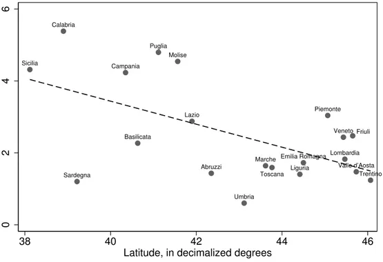
Figure 2 plots the relationship between the incidence of borrowing from friends and family against the latitude of the main city in the region in which the household resides. It shows that borrowing from friends and family is much more important in the South than in the North. It is highest in Calabria, and lowest in Umbria. This pattern is similar to that found for length of trials, which is inversely related to judicial efficiency.
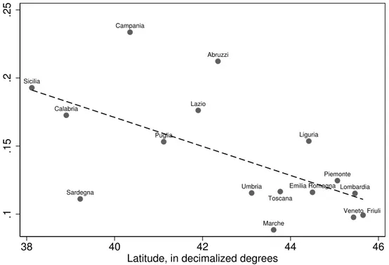
The Findomestic data records whether households default on their debts. Figure 3 plots the proportion of loans that defaulted in each region against its latitude. It clearly shows that relatively fewer households repay their debts in the South than in the North. In the North, under 10 percent of households fail to repay their debts on schedule, but in Calabria over 20 percent fail to repay on schedule: this rate is well over twice that in Trentino and Veneto, for instance. These figures suggest a positive relationship between the repayment of debts and the ease with which borrowers can be punished if they default, which the rest of the paper explores in more detail.
4
The econometric model
Our aim is to investigate the effect of access to informal credit markets, and of judicial en-forcement on borrower behaviour, and to provide evidence on the importance of asymmetric information in the Italian credit market. We estimate upper and lower bounds of the effect of judical enforcement and access to informal credit on repayment behaviour, and assess whether such households are more likely to apply for credit. To proceed, denote e as the repayment behaviour of the borrower taking the value 1 if the debt is repaid on schedule and
zero if any scheduled repayment is missed. Denote by X a vector of observable characteris-tics that might affect the repayment behaviour. The vectorX records the variables that the lender observes in making their credit granting decision and the additional variables that we have constructed. Finally, IG is a binary variable that takes the value one if the credit
request was granted, and zero if it was refused.
If the loan was granted we observe the repayment behaviour of the borrower. Our exercise is to test how the household’s characteristics affect whether the borrower defaults. However, we wish to deduce repayment behaviour accounting for the lending decision of our bank which requires us to predict the likely repayment behaviour of households whose loan application was refused. How does the repayment behaviour of Italian households change with their characteristics? Obviously, to do this we need to assume that households who apply for loans from our lender are typical of all Italian applicants, e.g. given their observable characteristics there is no difference between customers with our lender and customers who go elsewhere. This seems quite a strong assumption but can be consistent with economic theory. It will be true if, for instance, all lenders adopt the same strategy, conditional on the observable characteristics X. This seems reasonable if all firms are profit maximizing in a competitive market (or if they all have the same market power). It does rule out lenders segmenting the market and adopting different strategies. For instance, in the US, ‘sub-prime lenders’ concentrate on low-income / high risk households that are denied credit by more traditional lenders. However, these type of sub-prime lenders did not operate in the Italian credit market at this time. We believe that this assumption is reasonable, but if it is not, then although the results will not be applicable to the whole Italian credit market, they will be evidence of the behaviour of customers with our lender.
We also need to make an additional assumption if our results are representative of the whole Italian population: after accounting for the variables X, knowing that the agent has applied for a loan, does not predict whether it will be repaid. This is a much stronger assumption. It rules out that agents who are predictably bad borrowers are applying for credit.7 We will discuss this further below.
7Differences in the observable characteristics that can be controlled for by the lender are not evidence of
4.1
The selection problem
Our aim is to model the repayment behaviour of households. For any household with char-acteristicsX, their repayment probability is the sum of repayment if their credit application was granted multiplied by the probability of credit being granted, and repayment if it was refused multiplied by the probability of being refused credit.
E(e|X) = E(e|X, IG = 1|X)P r(IG= 1|X) +E(e|X, IG = 0|X)∗P r(IG = 0|X) (1)
We directly observe whether the household was granted credit, hence we knowP r(IG = 1|X)
and since the household is either granted or refused credit, we also know thatP r(IG= 0|X) =
1−P r(IG = 1|X). Since the household’s repayment behaviour is observed if it was granted
credit, we can also construct the sample analog ofE(e|X, IG = 1). However, the repayment
behaviour of households refused credit can not be directly observed hence we can not di-rectly construct E(e|X, IG = 0). This is the selection problem: some way must be found to
construct E(e|X, IG = 0) from what is observed, although we know it must lie between zero
and one. Notice that if rejected applicants are less likely to repay (implying that lenders screen out bad risks), the sample analog of E(e|X, IG= 1) underestimates E(e|X). There
are several standard econometric techniques to handle this type of selection problem, but each imposes economic assumptions. We now discuss the economic assumptions that are needed for identification.
4.1.1 Selection by observables, i.e.“Rubin”
In matching models, there is some set of variables, W, by which observations are sorted. Households with the same W are matched: households for which IG = 1 replace those
households, with the same W, for which IG= 0. Formally, this requires that:
e⊥IG|W
which implies thatP r(IG= 1|X, W, e) =P r(IG = 1|X, W).8 In our framework, this amounts
to requiring that the setW affects the credit scoring algorithm, but not repayment behaviour.
8Matching also requires the common support assumption to be satisfied. This implies that 0 <
This is unlikely to be satisfied by the data if the lender is rational and maximizes profits. Why would the lender use a variable in their screening procedure if it did not affect repay-ment behaviour? Hence this assumption seems inconsistent with lender rationality. However, it will be satisfied, if, for instance, the lender discriminates for non-economic reasons against subgroups in society (such as ethnic minorities) but this would be inconsistent with profit maximization.
4.1.2 Selection by unobservables, i.e.“Heckman”
A second popular method of solving the selection problem is through specifically modelling the selection process. Identification using this method requires some exclusion restriction (except in the case of identification via functional form assumptions). Formally, identification requires that for some set of variables W we have:
(a) E(e|X) =E(e|X, W)
(b) P r(IG= 1|W, X)6= Pr(IG = 1|X)
meaning that theW affects whether the application is rejected but not repayment. Assump-tions (a) and (b) are not very attractive. IfW enters the screening procedure, then as before, rationality implies that it is likely to affect repayment behaviour.
4.1.3 The bounds
Neither selection by unobservables nor matching seem to be consistent with profit maximizing by the lender. Both impose economic assumptions that are difficult to reconcile with lender rationality: lenders are likely to include variables in their screening procedure only if they predict likely repayment behaviour. However, if we make weaker assumptions, we can place bounds on the estimated effects of interest. Recall that we have modelled whether the household repays, e, as a binary variable equal to one if the debt is repaid on schedule, and zero if not. We can re-write equation 1 as:
P r(e = 1|X) = P r(e= 1|X, IG = 1)∗P r(IG = 1|X)
Recall that the data does not allow us to identify P r(e= 1|X, IG= 0): we cannot observe
whether households repay (or would have repaid) their loan if they were never granted credit. However, we know that the probability of repaying lies between zero and one, thus we can proceed as in Manski (1989), and place upper and lower bounds on the effect of the variables of interest. The lower bound assumes a zero probability of repaying for those who are refused credit, while the upper that this probability is one. This gives:
K0X =P r(e= 1|X, IG = 1)∗P r(IG = 1|X)
≤P r(e= 1|X)≤
P r(e= 1|X, IG= 1)∗P r(IG = 1|X) +P r(IG = 0|X) = K1X
(2)
That is, we define the lower bound as K0X and the upper bound as K1X. These bounds can
be identified since we have data on rejected applications, from which we can construct the probability that a credit application was granted, P r(IG = 1|X), and since we observe the
repayment behaviour of households granted credit we can construct P r(e= 1|X, IG= 1).
Suppose now that we want to measure the effect of access to informal credit markets, measured by the incidence of financial help from friends and family, on default rates. If one had point identification, the effect of family financial help is captured by the relevantβin the estimation of P r(e= 1|Xβ). Otherwise, we could split the sample by whether the reliance on family financial help is high (above median) or low. Defining Z = H if the reliance is high and Z =L if it is low, the difference in effort across high and low reliance is:
P r³e= 1|X, Z˜ =L´−P r³e= 1|X, Z˜ =H´
where we partition X into ˜X and Z. This probability is bounded between K1XL −K0XH
and K0XL−K1XH, where: K0XL = P r ³ e= 1|X, I˜ G = 1, Z =L ´ ∗P r³IG = 1|X, Z˜ =L ´ K1XL = P r ³ e= 1|X, I˜ G= 1, Z =L ´ ∗P r ³ IG= 1|X, Z˜ =L ´ + h 1−P r ³ IG= 1|X, Z˜ =L ´i K0XH = P r ³ e= 1|X, I˜ G = 1, Z =H ´ ∗P r ³ IG = 1|X, Z˜ =H ´ K1XH = P r ³ e= 1|X, I˜ G= 1, Z =H ´ ∗P r ³ IG= 1|X, Z˜ =H ´ + h 1−P r ³ IG= 1|X, Z˜ =H ´i
The intuition is simple. Suppose that the effect of Z on repayment is positive, then the smallest difference between a high value Z =H and a low value Z =L for access to credit
from family and friends Z is given by K1XL −K0XH. Here, K1XL represents the highest
possible value for the when Z =LwhileK0XH represents the lowest possible value for when
Z =H. In contrast the largest difference is given by K0XL−K1XH, the difference between
the lowest possible value when Z =L and the highest possible value when Z =H. Hence the difference in the estimated effect of whenZ is high, and whenZ is low, must be between
K1XL −K0XH and K0XL −K1XH. If, instead, the effect of Z is negative, K1XH −K0XL
becomes the lower bound, and K0XH −K1XL the upper bound.
4.1.4 Tightening the bounds
Suitable assumptions tighten the bounds, which could otherwise be large. Lenders have strong incentives to refuse credit to households which are less likely to repay their debts, hence households refused credit are likely to be worse credit risks. If this were not true then it would imply lenders were rejecting low risk and accepting high risk applicants, which would be inconsistent with their motive to screen customers, and with profit maximization. If rejected applicants are weakly less likely to repay their debts than households whose application was accepted then:
P r(e= 1|X, IG = 0)≤P r(e= 1|X, IG = 1)
Using this inequality means that equation (2) becomes:
P r(e = 1|X, IG= 1)∗P r(IG = 1|X)≤P r(e= 1|X)≤P r(e= 1|X, IG = 1) = ˜K1X (3)
which narrows the bounds, since the upper boundary, ˜K1X, is now tighter. With these
narrower bounds the effect of informal credit markets, measured by the extent of lending through friends and family, is instead bounded between ˜K1XL −K0XH and K0XL −K˜1XH
where:
˜
K1XL = P r(e= 1|X, IG = 1, Z =L)
˜
5
Estimation
In order to estimate the bounds one needs the sample analog of P r(e= 1|X, IG = 1) and
P r(IG= 1|X). We will use both a fully parametric estimator and a semi-parametric
esti-mator to construct these probabilities. Calculating the lower bound means estimating:
P r(e= 1|X, IG = 1)P r(IG = 1|X)
which is equivalent to estimating:
E(e·IG|X) (4)
That is, estimating the lower boundary is equivalent to estimating the proportion of house-holds who are both granted credit and repay that credit on time. While for the upper bound estimating:
P r(e= 1|X, IG = 1)P r(IG= 1|X) +P r(IG = 0|X)
is equivalent to estimating:
E(e·IG−IG|X) + 1 = 1−E(IG(1−e)|X) (5)
That is, estimating the lower boundary is equivalent to estimating one minus the proportion of households who are both granted credit and do not repay that credit on time. Lastly, the tightened upper bound is the probability that a household which is given credit repays their debt. This is the same as a naive estimate (which ignores selection) of the effect of the variable of interest on repayment behaviour. The upper, tightened upper and lower boundaries are easily calculated.
The parametric estimation of the lower, upper and tightened upper bound is straightfor-ward. We use standard probit regressions to provide the first set of results. Additionally, we estimate the lower, upper and tightened upper bound by using a semi-parametric approach. Probit regression is a maximum likelihood estimator which maximizes the function:
ΠiF(Xiβ)di[1−F(Xiβ)]1−di
wherediis a dummy variable which takes the value one if the event happens (for example,
otherwise. Probit regressions make parametric assumptions about both the functional form of the index function Xiβ and the distribution of the error term, assuming that F is the
normal distribution.
In order to free our estimates from distributional assumptions, we also employ a semi-parametric estimator. The lower bound is so estimated by minimizing the sample analog of:
keIG−E(eIG|X)k
where we approximateE(eIG|X) with a third order ploynomial in a linear index,Xβ. 9 This
procedure is similar to that suggested by Ichimura (1993), with two important differences. First, Ichimura employs kernel methods as approximation method while we favour series due to the large dimensionality of our problem. Second, while we are only interested in
E(eIG|X), Ichimura’s focus is on the estimation of β, which represents a more difficult task.
6
Results
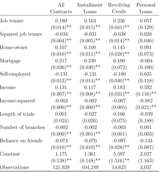
Table 1 presents estimates the probability of repayment among households granted credit by the bank. The first column reports results for all contract types together, while columns 2-4 report separate results for the three different types of contracts are offered: instalment credit, revolving credit and personal loans.
All regressions feature agency and year dummies, which implies that our estimates are not biased by unobservable regional or time effects.10 The results show that the probability
of repayment is an increasing and concave function of job seniority and income. This is consistent with the intuitive notion that wealthier households are less likely to default, though at a decreasing pace. The probability of not defaulting is also higher for home-owners and mortgage borrowers: these are typically stable income earners and the fact that they have
9Trying higher order polynomials does not affect the results. Consistency relies on the correlation between
the higher order terms and the error, defined aseIG−E(eIG|X), to vanish as the sample size grows.
10Agency dummies are defined on the basis of the province where the agency dealing with the contract is
a mortgage signals that they are good borrowers. The probability of repayment is instead lower for the self-employed. Their income is more volatile and risky and so these households are more likely to default.
Our measure of the quality of judicial enforcement, the average length of civil trials, does not affect the probability of repaying. But the proportion of households which repay their loans decreases significantly as reliance on friends and family for financial help increases. The degree of competition in the credit market, measured by the number of bank branches per banks in the province, is negatively correlated the proportion of households who repay. The results on enforcement are not entirely surprising, since consumer credit is unsecured and collateral is the main channel through which the quality of enforcement affects borrowers’ behaviour. The effect of access to credit from family and friends accords with the idea that those who have better outside options are more likely to default. Even if they are permanently excluded from the formal credit market, they can still borrow from friends and family in the informal credit market. The degree of competition, measured by the number of branches per bank in the province, is also significant. We interpret this result as reflecting that higher competition causes lenders to weaken credit standards, which reduces the average quality of the borrower and raisesex post default rates. These results are similar for each of the three different types of credit contract: the length of trial is not associated with reduced repayment for any of the different contract types whereas access to informal credit markets is significant for both installment loans and for revolving credit at the one percent level, and is significant at the 10 percent level in the last column. The number of branches per bank also remains significant for installment loans, but is no longer significant for either revolving credit or personal loans.
Nevertheless, table 1 gives as us a biased picture of the probability of repayment since it focuses only on those actually given credit. The probability of repayment if the household had been granted credit is not observed if the applicant is rejected. In order to draw inference on the probability of repayment, whether or not the application is rejected, we estimate the lower and the upper bounds.
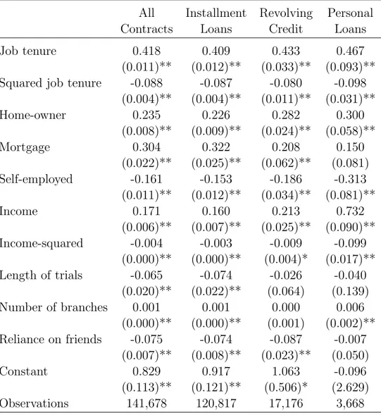
Table 2 provides probit an estimate of the lower bound. The lower bound is an increasing and concave function of job experience and income, decreases for self-employed and increases
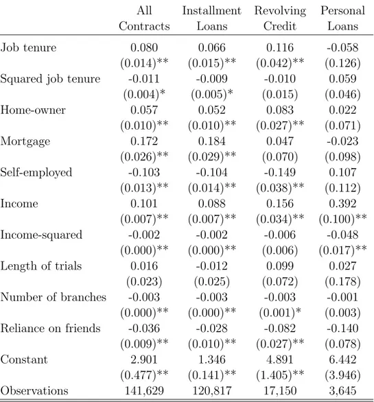
for home-owners. Having a mortgage makes the lower bound increase, while the degree of competition (measured by the number of branches), and the indicator of reliance on friends’ and relatives’ financial help are negatively related to the lower bound. The results are similar for each of the three different contracts. Table 3 shows the results for the upper bound. The first column refers to all contracts, the remaining three columns to instalment credit, revolving credit and personal loans. The results are similar to those in table 1. This is not surprising: the results in table 1 are the tightened upper bound, under the assumption that the non-rejected applicants are more likely to repay than the rejected ones.
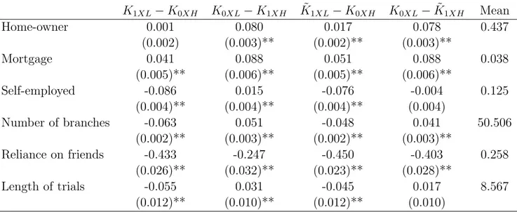
In order to understand the results, we explore how repayment changes if, say, the value of the index of reliance on friends’ and relatives’ financial help increases from the 25th to the 75th percentile of its distribution.
In table 4 we evaluate lower and upper bounds of the unobserved probability of defaulting at the 25th and 75th percentile for several variables. Two situations may arise: either the lower and upper bounds changes have the same sign, (both negative or both positive) or they have different signs. In the former instance we can identify the sign of the effect of the variable of interest, but in the latter case the sign of the effect is not identified.
Increasing access to credit from friends and family reduces the probability of repayment by between 25 percent (with a standard error of 3.2 percent) and 43 percent (with a standard error of 3.6 percent) or by between 40 (with standard error of 2.8) and 45 per cent (with standard error of 2.3) using the tightened bounds. This is substantial: the probability of repayment decreases by over 40 percent if access to credit from family and friends increases and everything else stays constant. It supports the hypothesis that the availability of informal credit weakens incentives to repay. The sign of the effect of length of trial is not identified. The effect is bounded between -0.05 and +0.03 using the wide bounds and between -0.05 and +0.02 using the tightened bounds. These effects are smaller, and we can not rule out that there is no effect, since zero lies between the upper and the lower bounds.
The effect of banks’ competition is also not identified. Increasing the number of branches per banks in the province form the 25th to the 75th percentile decreases the lower bound but increases the upper bound. Notice, however, that the changes in the probability of repaying are quite precisely estimated. Overall, the results do not rule out either a positive or a
negative effect of banking concentration on repayment.
Having a mortgage increases the probability of repayment by between 4.1 and 8.8 percent (between 5.1 and 8.8 percent using the tightened bound). Home-owners are more likely to repay by between 2 and 8 percent. Lastly, for the tightened bounds, we can rule out a positive effect for the self-employed since the probability of defaulting increases by between 0.4 and 7.6 percent.
6.1
Semi-parametric results
The results of our semi-parametric single index estimator are reported in table 5. Recall that we estimate both the parameters on the variables that enter the linear index, and the coefficients on a cubic polynomial in that index. The results show that the quadratic and the cubic terms are both significant at conventional significance levels when either the upper, the lower or the tightened upper bound is estimated. Using the parameter estimates reported in table 5 one can compute the lower, upper and tightened upper bound to the probability of repaying. The lower bound for the probability of not-defaulting is on average 73 percent, the upper bound 87, the tightened upper bound 85 percent.
The results are consistent with the probit estimates: the probability of repaying is an increasing and concave function of job tenure and income, is lower for self-employed and higher among those who own their house of residence or have a mortgage. The quality of judicial enforcement has a negative effect on the lower bound and a positive effect on the upper and the tightened upper bounds. This makes identification hard. In contrast, the number of branches, scaled by the number banks per province, increases the lower bound and reduces both the upper and the tightened upped bound. Lastly, the coefficient for availability of credit from family and friends reduces all the bounds.
As before, we quantify the effect of moving from the 25th percentile to the 75th percentile of each variable of interest. For access to credit from family and friends, the probability of defaulting increases by between 5 percent (with a standard error 2 percent) and 38 percent (with a standard error 1 percent) using the wide bounds, and by between 12 (with a standard error 2 percent) and 37 percent (with a standard error 2 percent), using the tightened upper
bound. These numbers confirm that the size of the effect is large, but smaller and perhaps more plausible than in the parametric case.
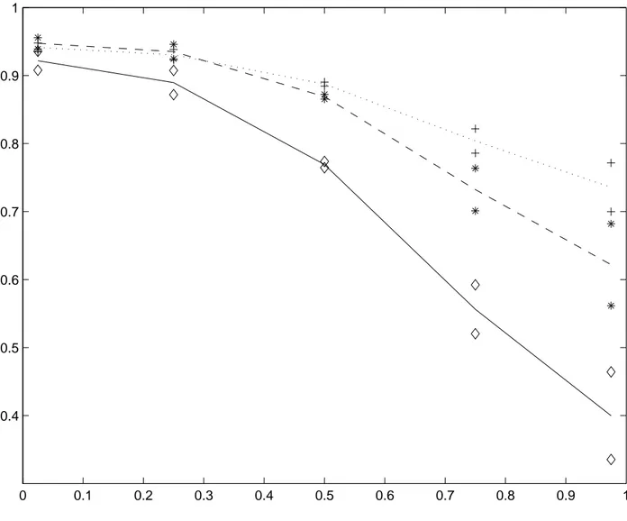
Figure 7 helps to visualize the effect of borrowing from relatives and friends on the probability of repaying. The solid line is the lower bound to the probability of repaying computed at the 2.5, the 25, the 50, the 75 and the 97.5 percentiles of the borrowing from family and relatives distribution, holding the other variables constant at their sample mean. The dotted and the dashed line are the upper and the tightened upper bounds and are obtained in a similar way. The figure shows that the lower, the upper and the tightened upper bounds decrease as financial help from family and friends increases. The decrease is sizable and statistically significant, as shown by the diamonds, the plus, and the stars placed two standard deviations above and below the lower, the upper and the tighten upper bound. The effect of judicial enforcement is more ambiguous. Figure 7 shows that upper and the tightened upper bounds increase with the length of trials, while the lower bound is flat. This implies that one cannot exclude that judicial enforcement does not affect the probability of repaying.
6.2
Adverse Selection and Moral Hazard
Our results show that the quality of judicial enforcement makes little difference to whether the borrower defaults or repays his loan. In contrast, access to credit from friends and family has large effects (the bounds exclude zero from the confidence interval). This large effect is consistent with theory. Recall that both Kehoe and Levine (1993) and Kocherlakota (1996) argued that incentives to repay depended on the punishment for default. For the small unsecured loans that our lender specializes in, the judicial process is relatively unimportant since it is rarely invoked. Instead, defaulters are punished by being denied further loans. Thus, if households have alternative credit sources (through informal credit markets provided by family and friends) then their incentives to repay debts in the formal market are much lower. We interpret it as evidence of moral hazard.
Our lender does not observe whether the household has access to alternative credit sources and thus does not change its lending behaviour to such households. But theory predicts and
we have found that these households are less likely to repay their debts on schedule. This implies moral hazard: incentives to repay depend on access to these informal credit markets. However, this is not the same as moral hazard in Jaffee and Russell (1976), in which granting credit changes behaviour. Instead, we have found that access to alternative credit sources affects repayment. Moral hazard arises because the bank cannot write a contract, conditional on whether the household has access to informal credit markets, and hence cannot exploit the information that those with access to family and friends financial help are more likely to default. Nevertheless, this is compelling evidence for moral hazard in consumer credit markets.
What does this say about adverse selection? Recall that adverse selection means that households who are predictably worse credit risks are more likely to apply for credit, after conditioning on the characteristics that the bank observes. We know that households who have access to informal credit markets are more likely to default, and we know that the lender does not observe whether potential borrowers have access to alternative sources of credit. Hence to establish adverse selection we need only to establish whether these households are more likely to apply for, and be granted, credit in the formal sector. This would be unambiguous evidence of adverse selection.
Formally, we wish to show that family and friends financial help is more prevalent in the Findomestic population than in the general household population. In order to do that, we matched the Findomestic sample with the SHIW sample, which is a representative sample of the Italian household population, and then we check if the average reliance on family and friends financial help is different between the two samples.11 The two samples are matched
along three variables, number of kids, marital status and geographic area of residence.12 This
implies that the two samples are balanced with respect these three variables: their mean is the same in the Findomestic and SHIW sample.
The results show that households with access to informal credit are 0.3 percent more likely to apply for and be granted credit. This is highly statistically significant (the t-statistic is
11This is like estimating the average treatment effect, where households surveyed in the Findomestic are
treated and those in SHIW are non treated.
over 30).13 Since around 3 percent of Italian households borrow from family and friends, we
see this result as also economically significant. Overall, this suggests that adverse selection is also present in our population.
7
Conclusion
Using a leading Italian lender’s administrative data on credit applications, we are able to assess how features of the market affect repayment behaviour. Two issues are particularly important: how easy it is to enforce debts through the courts; whether the agents have alternative credit sources. We measure judicial enforcement with the average length of civil trials, while we use credit from friends and family to measure the availability of informal sources of credit. We also measure competition using the total number of bank branches in each province. Identifying the effects of these variables is not trivial. A selection issue arises because we do not observe the repayment behaviour of those households which are refused credit by our lender. Two popular methods for addressing selection require imposing the economic restriction that the lender’s screening procedure is unrelated to the potential borrowers repayment behaviour, which is unlikely to be satisfied. At the cost of losing point identification, we impose less stringent assumptions and provide upper and lower bounds of the likely effect of the variables of interest.
The effect of informal credit markets on whether the debt was repaid is both economically and statistically significant. This evidence is consistent with the predictions of Kehoe and Levine (1993) and Kocherlakota (1996), that repayment behaviour depends crucially on how default is punished. Borrowing from family and friends improves household’s outside option and reduces the penalty for default. Households with access to these informal credit markets view exclusion from the formal credit market as less onerous since they can still borrow from friends and family should the need arrive. In contrast, the effect of judicial enforcement is economically small (one tenth of the effect of family and friends) and statistically insignifi-cant. This is unsurprising given the small size of the typical loan that we examine, and the
13Finding that Findomestic households are less likely to rely on family and friends financial help would
fact that these loans are uncollateralized.
Our data also allows us to discuss asymmetric information. We observe an extra variable that the lender does not observe, which predicts whether the borrower defaults. This extra variable measures access to credit from family and friends and can be used to explore adverse selection. Our results suggest that moral hazard is present in the formal credit market, in the sense that access to credit from family and friends reduces repayment in the formal sector. However, unlike conventional moral hazard where the loan from the lender changes repayment behaviour on that loan, we instead show that access to alternative credit sources changes repayment behaviour on the loan granted by the lender. Because we use administrative data, we know that access to credit from family and friends does not enter the lending decision, and hence does not affect lender behaviour. Hence, a test for adverse selection is whether households with access to these informal sources of credit are more likely to apply for (and be granted) credit by our lender. The results show that such households are 0.3 percent more likely to have credit, which is both statistically and economically significant.
References
[1] Alessie, Rob, Stefan Hochguertel, and Guglielmo Weber, (2005), “Consumer Credit: Evidence from Italian Micro Data,” Journal of the European Economic Association, 3, pp. 144-178
[2] Ausubel, Lawrence, (1999), “Adverse Selection in the Credit Card Market,” mimeo, University of Maryland.
[3] Banerjee Abhijit, and Newman, Andrew, (1998) “Information, the Duel Economy, and Development”Review of Economic Studies, 65, pp.631-653.
[4] Casolaro, Luca, Gambacorta Leonardo and Luigi Guiso, (2005), “Regulation, Formal and Informal Enforcement and the Development of Household Loan Market: lessons from Italy”, in The Economics of Consumer Credit, ed. by Giuseppe Bertola, Richard Disney and Charles Grant, MIT press, Cambridge, MA.
[5] Chiappori, Pierre-Andr´e and Bernard Salani´e, (2003), “Testing Contract Theory: A Survey of Some Recent Work,” in Advances in Economics and Econometrics, vol 1, M. Dewatripont, L. Hansen and S. Turnovsky eds, Cambridge University Press.
[6] Chiappori, Pierre-Andr´e and Bernard Salani´e, (2000), “Testing Asymmetric Information in Insurance Markets,” Journal of Political Economy,108, pp. 56-78.
[7] Chiappori Pierre-Andr´e, Jullien, Bruno, Salani´e Bernard and Fran¸cois Salani´e, (2005), “Asymmetric Information in Insurance: General Testable Implications,” forthcoming in the Rand Journal of Economics.
[8] DiNardo, John, Fortin, Nicole M. and Thomas Lemieux (1996) “Labor Market In-stitutions and the Distribution of Wages, 1973-1992: A Semiparametric Approach”,
Econometrica, 64(5), 1001-1044.
[9] Edelberg, Wendy, (2003), “Risk-based pricing of interest rates in household loan mar-kets,” FEDS Working Paper No. 2003-62.
[10] Fabbri, Daniela and Mario Padula, (2004), “Does Poor Legal Enforcement Make House-holds Credit-Constrained?,” Journal of Banking and Finance, 28(10), pp. 2369-2397.
[11] Fay, Scott, Hurst, Erik, and Michelle White (2002), “The Household Bankruptcy Deci-sion”, American Economic Review, 92(3), pp. 706-718.
[12] Ghosh, Parikshi, Mookherjee, Dilip and Debray Ray, (2000), “Credit rationing in devel-oping countries: an overview of the theory,” in A Reader in Development Economics, edited by Dilip Mookherjee and Debraj Ray, London: Blackwell
[13] Guiso, Luigi, Sapienza Paola and Luigi Zingales, (2004) “Does Local Financial Devel-opment Matter?” Quarterly Journal of Economics, 119, pp. 929-969.
[14] Jaffee, Dwight, M., and Tom Russel, (1976), “Imperfect information, uncertainty, and credit rationing,” Quarterly Journal of Economics, 80, pp. 651-666.
[15] Jappelli, Tullio, Pagano Marco and Magda Bianco, (2005),“Courts and Banks: the Ef-fect of Judicial Enforcement in Credit Markets,”Journal of Money Credit and Banking, 37(2) pp. 223-245.
[16] Ichimura, Hideiko, (1993), “Semiparametric Least Squares (SLS) and Weighted SLS Estimation of Single-Index Models,” Journal of Econometrics, 58, pp. 71-120.
[17] Karlan, Dean S. and Jonathan Zinman, (2005), “Observing Unobservables: Identifying Information Asymmetries with a Consumer Credit Field Experiment,” paper presented at Finance & Consumption conference: The Micro Foundations of Credit Contracts, 21 and 22 May 2004, Florence
[18] Kehoe, Timothy J., and David K. Levine, (1993), “Debt-Constrained Asset Markets,”
Review of Economic Studies, 60, pp. 865-888.
[19] Kocherlakota, Narayana, (1996), “Implications of efficient risk sharing without commit-ment”, Review of Economic Studies, 63, pp. 595-609.
[20] Klonner, Stefan, and Ashok Rai (2005), “Adverse Selection in Credit Markets: Evidence from South Indian Bidding Roscas”, mimeo, Cornell University.
[21] Manski, Charles, (1989), “The anatomy of selection problem,” Journal of Human Re-sources, 24, pp. 343-360
[22] Manski, Charles, (1990), “Nonparametric bounds on treatment effects,”American Eco-nomic Review, 80, pp. 319-323
[23] Rosenbaum, Paul R., and Donald B. Rubin (1983) “The Central Role of the Propensity Score in Observational Studies for Causal Effects”, Biometrika 70(1), pp. 41-55
[24] Stiglitz, John E., and Andrew Weiss, (1981), “Credit rationing in markets with imperfect information,” American Economic Review, 71, pp. 393-410.
CALTANISSETTA CATANIA REGGIO C. PALERMO MESSINA CATANZARO CAGLIARI LECCE NAPOLI TARANTO POTENZA SALERNO SASSARI BARI CAMPOBASSO ROMA AQUILA PERUGIA ANCONA FIRENZE GENOVABOLOGNA BRESCIA TORINO VENEZIA MILANO TRIESTE TRENTO BOLZANO 1.5 2 2.5 3 38 40 42 44 46
Latitude, in decimalized degrees
Piemonte Valle d’Aosta Lombardia Trentino Veneto Friuli Liguria Emilia Romagna Toscana Umbria Marche Lazio Abruzzi Molise Campania Puglia Basilicata Calabria Sicilia Sardegna 0 2 4 6 38 40 42 44 46
Latitude, in decimalized degrees
Piemonte Lombardia Veneto Friuli Liguria Emilia Romagna Toscana Umbria Marche Lazio Abruzzi Campania Puglia Calabria Sicilia Sardegna .1 .15 .2 .25 38 40 42 44 46
Latitude, in decimalized degrees
0 0.1 0.2 0.3 0.4 0.5 0.6 0.7 0.8 0.9 1 0.4 0.5 0.6 0.7 0.8 0.9 1
0 0.1 0.2 0.3 0.4 0.5 0.6 0.7 0.8 0.9 1 0.7 0.75 0.8 0.85 0.9 0.95
Table 1: The probability of not-default among those given credit All Installment Revolving Personal Contracts Loans Credit Loans Job tenure 0.180 0.163 0.236 0.057 (0.014)** (0.015)** (0.041)** (0.129) Squared job tenure -0.034 -0.031 -0.038 0.028
(0.004)** (0.005)** (0.014)** (0.046) Home-owner 0.107 0.100 0.145 0.091 (0.010)** (0.011)** (0.028)** (0.073) Mortgage 0.217 0.230 0.100 -0.004 (0.026)** (0.030)** (0.072) (0.100) Self-employed -0.131 -0.131 -0.180 0.035 (0.013)** (0.014)** (0.040)** (0.118) Income 0.131 0.117 0.183 0.592 (0.007)** (0.008)** (0.031)** (0.116)** Income-squared -0.003 -0.002 -0.007 -0.082 (0.000)** (0.000)** (0.005) (0.021)** Length of trials 0.001 -0.027 0.106 -0.039 (0.024) (0.026) (0.075) (0.188) Number of branches -0.002 -0.002 -0.003 0.001 (0.000)** (0.001)** (0.001) (0.003) Reliance on friends -0.074 -0.070 -0.097 -0.144 (0.010)** (0.010)** (0.028)** (0.087) Constant 1.175 1.361 5.597 2.027 (0.138)** (0.148)** (1.516)** (1.163) Observations 121,928 104,249 14,625 3,037
Standard errors in parenthesis. ?significant at 5 percent level, ??significant at 1 percent level.
The regression also included a full set of provincial and year dummies. Income is in 10,000 Euros.
Table 2: The lower bound of the probability of not-defaulting All Installment Revolving Personal Contracts Loans Credit Loans Job tenure 0.418 0.409 0.433 0.467
(0.011)** (0.012)** (0.033)** (0.093)** Squared job tenure -0.088 -0.087 -0.080 -0.098
(0.004)** (0.004)** (0.011)** (0.031)** Home-owner 0.235 0.226 0.282 0.300 (0.008)** (0.009)** (0.024)** (0.058)** Mortgage 0.304 0.322 0.208 0.150 (0.022)** (0.025)** (0.062)** (0.081) Self-employed -0.161 -0.153 -0.186 -0.313 (0.011)** (0.012)** (0.034)** (0.081)** Income 0.171 0.160 0.213 0.732 (0.006)** (0.007)** (0.025)** (0.090)** Income-squared -0.004 -0.003 -0.009 -0.099 (0.000)** (0.000)** (0.004)* (0.017)** Length of trials -0.065 -0.074 -0.026 -0.040 (0.020)** (0.022)** (0.064) (0.139) Number of branches 0.001 0.001 0.000 0.006 (0.000)** (0.000)** (0.001) (0.002)** Reliance on friends -0.075 -0.074 -0.087 -0.007 (0.007)** (0.008)** (0.023)** (0.050) Constant 0.829 0.917 1.063 -0.096 (0.113)** (0.121)** (0.506)* (2.629) Observations 141,678 120,817 17,176 3,668
Standard errors in parenthesis. ?significant at 5 percent level, ??significant at 1 percent level.
The regression also included a full set of provincial and year dummies. Income is in 10,000 Euros.
Table 3: The upper bound of the probability of not-defaulting All Installment Revolving Personal Contracts Loans Credit Loans Job tenure 0.080 0.066 0.116 -0.058 (0.014)** (0.015)** (0.042)** (0.126) Squared job tenure -0.011 -0.009 -0.010 0.059
(0.004)* (0.005)* (0.015) (0.046) Home-owner 0.057 0.052 0.083 0.022 (0.010)** (0.010)** (0.027)** (0.071) Mortgage 0.172 0.184 0.047 -0.023 (0.026)** (0.029)** (0.070) (0.098) Self-employed -0.103 -0.104 -0.149 0.107 (0.013)** (0.014)** (0.038)** (0.112) Income 0.101 0.088 0.156 0.392 (0.007)** (0.007)** (0.034)** (0.100)** Income-squared -0.002 -0.002 -0.006 -0.048 (0.000)** (0.000)** (0.006) (0.017)** Length of trials 0.016 -0.012 0.099 0.027 (0.023) (0.025) (0.072) (0.178) Number of branches -0.003 -0.003 -0.003 -0.001 (0.000)** (0.000)** (0.001)* (0.003) Reliance on friends -0.036 -0.028 -0.082 -0.140 (0.009)** (0.010)** (0.027)** (0.078) Constant 2.901 1.346 4.891 6.442 (0.477)** (0.141)** (1.405)** (3.946) Observations 141,629 120,817 17,150 3,645
Standard errors in parenthesis. ?significant at 5 percent level, ??significant at 1 percent level.
The regression also included a full set of provincial and year dummies. Income is in 10,000 Euros. Squared income and the number of branches per banks are divided by 10.
Table 4: Changes in the probability of defaulting: parametric estimates K1XL−K0XH K0XL−K1XH K˜1XL−K0XH K0XL−K˜1XH Mean Home-owner 0.001 0.080 0.017 0.078 0.437 (0.002) (0.003)** (0.002)** (0.003)** Mortgage 0.041 0.088 0.051 0.088 0.038 (0.005)** (0.006)** (0.005)** (0.006)** Self-employed -0.086 0.015 -0.076 -0.004 0.125 (0.004)** (0.004)** (0.004)** (0.004) Number of branches -0.063 0.051 -0.048 0.041 50.506 (0.002)** (0.003)** (0.002)** (0.003)** Reliance on friends -0.433 -0.247 -0.450 -0.403 0.258 (0.026)** (0.032)** (0.023)** (0.028)** Length of trials -0.055 0.031 -0.045 0.017 8.567 (0.012)** (0.010)** (0.012)** (0.010)
Bootstrap standard errors in parenthesis. ?means significant at 5 percent level,??significant at
1 percent level. The last column reports the means of the variables given in left-hand column. The length of trials is expressed in years.
Table 5: Semi-parametric estimates of the bounds on the the probability of not-defaulting. Tightened
Lower Bound Upper Bound Upper Bound Index coefficients
Job tenure 0.167 0.032 0.053
(0.009)** (0.005)** (0.005)** Squared job tenure -0.038 -0.004 -0.009
(0.002)** (0.001)** (0.001)** Home-owner 0.076 0.019 0.029 (0.005)** (0.004)** (0.003)** Mortgage 0.098 0.075 0.068 (0.009)** (0.013)** (0.010)** Self-employed -0.048 -0.033 -0.034 (0.004)** (0.006)** (0.005)** Income 0.069 0.046 0.048 (0.004)** (0.003)** (0.003)** Income-squared -0.002 -0.001 -0.001 (0.000)** (0.000)** (0.000)** Length of trials -0.006 0.035 0.022 (0.006) (0.008)** (0.007)* Number of branches 0.001 -0.001 -0.000 (0.000)** (0.000)** (0.001)** Reliance on friends -0.015 -0.008 -0.013 (0.001)** (0.001)** (0.001)** Polynomial coefficients (Xβ)2 0.781 0.264 0.766 (0.185)** (0.099)** (0.182)** (Xβ)3 -0.850 -0.368 -0.814 (0.199)** (0.087)** (0.193)** Observations 141,678 141,629 121,928
Standard errors in parenthesis. ?means significant at 5 percent level,??significant at 1 percent
level. The regression is run for all contracts together, and includes a full set of provincial and year dummies. Income refers to disposable annual income measured in 10,000 Euros. The
estimates were obtained by choosing the parameters that minimizesε0εwhere ε=y−f(Xβ)
Table 6: Robustness checks: probability of applying
Borrowers Discouraged borrowers 1995 and 1995,1998 1995 and 1995,1998 1998 SHIW and 2000 SHIW 1998 SHIW and 2000 SHIW
Length of trials 0.018 0.002 -0.017 -0.004 (0.017) (0.009) (0.011) (0.005) Reliance on friends 0.060 0.072 0.095 0.059 (0.013)** (0.009)** (0.008)** (0.006)** Constant 0.289 0.270 0.070 0.052 (0.112)** (0.056)** (0.044) (0.034) Observations 15,148 23,283 14,103 21,932
Standard errors in parenthesis. ?significant at 5 percent level, ??significant at 1 percent level.
The regression included a full set of provincial and year dummies, as well as the variables, age and its square, income and its square home-ownership, whether the household has mortgage, the head is a self-employed.