D
S
E
Working
Paper
ISSN: 1827/336X
Multiple Lending and
Constrained Efficiency
in the Credit Market
Andrea Attar
Eloisa Campioni
Gwenaël Piaser
Dipartimento
Scienze Economiche
Department
of Economics
Ca’ Foscari
University of
W o r k i n g P a p e r s D e p a r t m e n t o f E c o n o m i c s C a ’ F o s c a r i U n i v e r s i t y o f V e n i c e N o . 2 9 / W P / 2 0 0 6 ISSN 1827-336X T h e W o r k i n g P a p e r S e r i e s i s a v a i l b l e o n l y o n l i n e w w w . d s e . u n i v e . i t / p u b b l i c a z i o n i F o r e d i t o r i a l c o r r e s p o n d e n c e , p l e a s e c o n t a c t : w p . d s e@ u n i v e . i t D e p a r t m e n t o f E c o n o m i c s C a ’ F o s c a r i U n i v e r s i t y o f V e n i c e C a n n a r e g i o 8 7 3 , F o n d a m e n t a S a n G i o b b e 3 0 1 2 1 V e n i c e I t a l y F a x : + + 3 9 0 4 1 2 3 4 9 2 1 0
Multiple Lending and Constrained Efficiency in the Credit
Market
Andrea Attar
IDEI, University of Toulouse and Università di Roma, La Sapienza
Eloisa Campioni
LUISS, University of Rome
Gwenaël Piaser
University of Venice
Abstract
This paper studies the relationship between competition and incentives in an economy with financial contracts. We concentrate on non-exclusive credit relationships, those where an entrepreneur can simultaneously accept more than one contractual offer. Several homogeneous lenders compete on the contracts they offer to finance the entrepreneur's investment project. We model a common agency game with moral hazard, and we characterize its equilibria. As expected, notwithstanding the competition among the principals (lenders), non-competitive outcomes can be supported. In particular, positive profit equilibria are pervasive. We then provide a complete welfare analysis and show that all equilibrium allocations turn out to be constrained Pareto efficient.
Keywords
Common Agency, Financial Markets, Efficiency
JEL Codes
D4, D6, G2
Address for correspondence: Gwenaël Piaser Department of Economics Ca’ Foscari University of Venice Cannaregio 873, Fondamenta S.Giobbe 30121 Venezia - Italy Phone: (++39) 041 234 91 22 Fax: (++39) 041 2349176 e-mail: [email protected] This Working Paper is published under the auspices of the Department of Economics of the Ca’ Foscari University of Venice. Opinions expressed herein are those of the authors and not those of the Department. The Working Paper series is designed to divulge preliminary or incomplete work, circulated to favour discussion and comments. Citation of this paper should consider its provisional character.
1
Introduction
The paper is devoted to the analysis of credit markets where several lenders strategi-cally compete over the contracts they offer to entrepreneur-borrowers. At the stage of contracting, the decision of the unique borrower crucially depends on the loans she is si-multaneously receiving from all the lenders of the economy. We consider a set-up where
the contracts are non-exclusive, i.e. the borrower is allowed to accept more than one
contract at a time. The main aim of the work is to emphasize the interplay of contrac-tual externalities in determining the welfare properties of the equilibria arising in such framework.
Examples of financial interactions with non-exclusive contracting which aim at clarify-ing the relationship between incentives and competition are very recent: the main general results and implications are discussed by Segal & Whinston (2003).
The relevant finding of the literature on non-exclusivity can be summarized as follows: the contractual externalities emerging when several principals interact with one common
agent, can be responsible for existence ofsecond-best inefficient equilibria. In other words,
a social planner who is subject to incentive constraints and feasibility can achieve outcomes that Pareto dominate the equilibrium outcomes of players’ interactions.
Constrained inefficient equilibria have mostly been analyzed in insurance set-ups (Arnott & Stiglitz (1993), Hellwig (1983), Kahn & Mookherjee (1998) and Bisin & Guaitoli (2004)). The present essay proposes an investigation on the welfare properties of equilibria in the credit market, where strategic competition is over financial contracts.
The theoretical contributions examining credit market imperfections mostly use the principal-agent model as a tool to represent credit relationships. The solution to a standard principal-agent program is equivalent to the outcome of a planner’s maximization problem under exclusive contracting and subject to the same asymmetry of information, given appropriate welfare weights.
Exclusivity clauses are not explicitly imposed, though, in several financial relationships. It is recognized that many firms have access to multiple credit sources, as shown by Petersen & Rajan (1995) for the small firms in the U.S., or by Detragiache et al. (2000) for the Italian case. The credit card market has been proposed as an example of non-exclusive dealings, as Bizer & DeMarzo (1992) and Parlour & Rajan (2001) have already explained. Hence, enriching the analysis of competition in the credit market using the common agency approach to financial contracting, we believe is a necessary step to analyze competition on financial markets and the welfare properties of the equilibria of the corresponding game. This work could then be regarded as part of a research project on welfare foundations for policy intervention, in particular along the lines of the credit channel of monetary policy.1
1The credit view of monetary policy relates the effects of a monetary intervention to the difficulties
for borrowers to access the credit market. Fundamental imperfections in credit relationships, mainly due to asymmetric information problems, constitute the main channel for monetary transmission. Many have been the contributions to the theoretical assessment of this transmission mechanism (see Besanko & Kanatas (1993), Bolton & Freixas (2000), Holmstrom & Tirole (1997) and Repullo & Suarez (2000)). The standard models of the credit channel assume perfect competition among investors in the financial market; thus, they restrict the analysis to zero-profit equilibria for lenders in an economy subject to asymmetric
We propose a simple, static and partial equilibrium model of the credit market to study multiple credit relationships. We model competition between an arbitrarily large and finite number of lenders who offer credit lines to a single borrower. The borrower has to take some non-observable action; she can choose not to perform the hidden action and to divert resources for private use, in which case she will appropriate a fixed proportion
of the received liquidity.2 By exerting effort in the investment project, she will get some
stochastic returns from the production technology. None of the lender is irrelevant, in the sense that every proposed loan affects the entrepreneur on the effort she will choose.
The possibility to sign several contracts simultaneously generates externalities among the financiers. These externalities are responsible for the emergence of equilibrium results which are not in line with Bertrand theory of competition. If the agency costs are high enough, competition among financiers delivers non-competitive results in the forms of credit rationing and of positive extra-profits at equilibrium.
The model is closely related to the Parlour & Rajan (2001)’s work on the credit cards market, which we regard as a useful benchmark to provide insights on the emergence of positive profit equilibria. We modified their analysis, generalizing their incentive structure. As a result, we are able to provide the same equilibrium characterization as Parlour & Rajan (2001) in a richer set-up.
The main contribution of this work relies, though, on the welfare analysis of the credit market equilibria. Examining this issue, we show that every positive-profit equilibrium is constrained Pareto efficient, i.e. it would be the outcome of the decision of a central authority subject to the same informational constraints. The result is not in line with the main findings of the existing literature on competition and incentives, which has always emphasized that non-exclusive contracting generates those externalities sustaining
constrained inefficient outcomes.3
Our simple example clarifies how could the incentive structure eliminate the (con-strained) inefficiency result. The crucial element turns out to be the existence of a bind-ing Incentive Compatibility constraint in every credit market equilibrium. This guarantees that all equilibrium outcomes can in fact be obtained as the solution of a planner’s prob-lem. In particular, the feasible sets of the two problems result to be the same.
Surprisingly, the same argument applies to the recent literature on insurance mar-kets with non-exclusive contracting. Relaxing the assumption of risk-averse agents in the framework of Bisin & Guaitoli (2004) and Kahn & Mookherjee (1998) implies that their positive profits equilibria (which were the inefficient ones) would feature binding incentive constraints and, as a consequence, collapse to allocations on the second-best frontier. information. In the optimal contracting problems, this is summarized in a binding Individual Rationality constraint for the (single) financier. Now, if lenders compete on the loan contracts they offer to borrowers, then they could strategically exploit each others presence and positive-profit equilibria may appear. The existence of a credit channel of monetary policy in such a context has not been analyzed in the literature, so far.
2
This model is indeed compatible with the literature on strategic default. For a detailed justification of such an approach to strategic default, refer to Parlour & Rajan (2001).
3
See Arnott & Stiglitz (1993), Kahn & Mookherjee (1998), Bisin & Guaitoli (2004), Segal & Whinston (2003).
The discussion is organized in the following way: Section 2 presents the features of our set-up. Section 3 characterizes the credit market equilibria of a simplified version of the model. Section 4 provides the welfare analysis and the results on the efficiency of the positive-profit equilibria as compared to those obtained in the insurance set-ups. Section 5 presents a discussion of our results in the light of the existing literature on competitive insurance markets under moral hazard. The Appendix presents the general version of our credit economy and contains all the proofs.
2
The model
Credit relationships are represented in a simple way. In this economy there are N ≥ 2
lenders (indexed byi∈N ={1,2, ..., N}) who compete over the loan contracts to finance
a single borrower.4 The entrepreneur is penniless though she has access to the technology
for the production of the only existing good. Contractual offers are simultaneous. Having received all the contract’s proposals, the borrower decides which of them to sign taking
into account that she can accept any subset of them.5
The production process is stochastic and the probability distribution over the random outcomes is determined by the entrepreneur’s choice on a non-contractible action (effort).
The entrepreneur’s effort space is made of two elements: eH and eL, with eH > eL. If
the high efforteH is chosen, production successfully yieldsG(I) for every I invested with
probabilityp and 0 with probability 1−p. If, on the contrary, the low effort eL is taken,
the entrepreneur’s activity is unsuccessful with probability 1.
Exerting effort implies some disutility for the borrower. We chose to represent this feature using a private benefit functionψ(e), which takes values ψ(eH) = 0 and ψ(eL) =
B(I). The private benefit function B(I) is assumed continuous, increasing and convex
and such to satisfy the Inada conditions. For the discussion that follows, we adopt a linear version of the private benefit function, i.e. B(I) =BI.6
In other words, we are considering the set of outcomes Y = {G(I),0}. The private
choice of effort affects the probability distribution of these realizations. In particular, if the entrepreneur exerts high efforteH, the probability vector is given by the array: {p,1−p}
with p > 0. If instead the entrepreneur shirks, i.e. chooses low effort eL, the lottery is
degenerate and equal to {0,1}. The production function G(I) is continuous, increasing
and strictly concave inI. Inada conditions are also satisfied.
Let us describe the normal form of the game we are considering. Lenders strategically
compete over financial contracts. The strategy of each lenderiis the choice of the contract
Ci. The contract offer Ci prescribes a repayment lineRi and a loan amount Ii, i.e.
Ci = (Ri, Ii)∈ Ci⊆R 2
+
4
Abusing notation we indicate the set of lenders and its cardinality withN.
5
This defines a scenario ofdelegated common agency Martimort & Stole (2003)
6
This is without loss of generality and keeps the problem simple. In the Appendix we consider the more general version of the model.
whereCi is the set of feasible contract offers for each lender i. We also denoteC=iCi
the aggregate set of offered contracts.7 The borrower’s strategy is therefore given by the
map:
sb :C → {0,1}N
eH, eL
With a small abuse of notation, we also define the generic element of the set{0,1}N as the arrayab = a1b, a2b, ..., aNb
, where ai
b={0,1} is the borrower’s decision of rejecting or
accepting lenderi’s offer. The choice of the array ab defines the set of accepted contracts
A:
A=
i∈N :aib = 1
In other words, the borrower decides on the choice of the effort level and on the relevant set of offers to accept. Her strategy set will be denoted as Sb, so thatsb ∈ Sb.
Let us now consider the payoffs of this game. The borrower’s payoff is given by:
πb=
(
p[G(I)−R] if eH is chosen
BI ifeL is chosen
whereR and I denote the aggregate repayment and investment, respectively:
R=X i∈A Ri and I = X i∈A Ii.
Lender i’s payoff is given by:
πi=
(
pRi−(1 +r)Ii ifCi is accepted
0 otherwise,
and r∈R+ is the lender’s cost of collecting deposits.
8
Observe that lender i’s payoff does not directly depend on lenderj’s strategies.
Exis-tence of contractual externalities among lenders is originated by the borrower’s behavior
only: at the stage of contracting with lender i, the action chosen by the borrower also
depends on the contractual offer she is receiving from each lenderj6=i.9
The borrower is subject to limited liability. If the low effort is chosen, she will have no
appropriable resources to repay the loan. In particular each lenderiwill earn a negative
pay-off of:
7
One should notice that lenders’ strategy are take-it or leave-it offers. When common agency games of
completeinformation are considered, this restriction on principals’ strategy spaces involves a loss of gener-ality. If principals are allowed to offer menus over the relevant alternatives, there can emerge equilibrium outcomes that could not be supported by simple offers (see Peters (2001) and Martimort & Stole (2002)). There is, anyway, always a rationale for the use of take-it or leave-it offers: Peters (2003) shows that every equilibrium outcome of this simple game continues to be an equilibrium outcome of the extended game where principals are competing over menus.
8Lenders here rely on the deposit market to finance entrepreneurial activity. 9
This is usually referred to as the absence of direct externalities among principals. Most common agency models have been developed in such a simplified scenario. Examples of recent researches where direct externalities among principals are considered include Bernheim & Whinston (1998) and Martimort & Stole (2003).
πi=−(1 +r)Ii.
The only way to give the financier a positive repayment will hence be to induce the high effort choice. We model credit market interactions as a sequential game, with a first stage where several lenders play a simultaneous move game and a second stage where the borrower decides on acceptance/rejection of each offer and finally exerts effort. In formal terms, loan relationships are represented by the following complete information common agency game Γ:
Γ ={(πi)i∈N, πb,C,Sb}.
3
Credit market equilibria
This section discusses the properties of the Subgame Perfect Nash Equilibria of the game Γ. The equilibria match those discussed by Parlour & Rajan (2001). However, we are able to show that the specific characterization obtained in Parlour & Rajan (2001) can in fact be reproduced in a more general setting, where the private benefit earned by the single
agent is taken to be a non-linear function of the amount borrowedI.
The discussion of this general case is left to the Appendix (that contains all the proofs),
while in the following sections we present the simpler case with B(I) =BI, with B >0.
This scenario indeed simply reformulates the original Parlour & Rajan (2001) model in a moral hazard setting and introduces a positive interest rate on deposits.
Having presented the equilibria of the credit market we will characterize the constrained Pareto frontier of the economy, and show that competition among lenders sustains only second-best efficient allocations (equilibria). We start by remarking that whenever the
efforteL is chosen, every active lender earns negative profits. As a consequence, at
equi-librium only the high level of effort will be implemented.
Furthermore, since the entrepreneur’s private benefit is monotonically increasing in
the aggregate lendingI, the borrower will always have the incentive to accept the whole
array of offered contracts when selectingeL. This greatly simplifies the incentive analysis. We consider Subgame Perfection as the relevant equilibrium concept for the game Γ.
Definition 1 A (pure strategy) Subgame Perfect equilibrium(SP E) of the game Γ is an array hR˜i,I˜i i∈N,(˜a i b)i∈N, p i such that:
the borrower is optimally choosing the set of accepted contracts A(i.e. she is selecting
her optimal array ab∈ {0,1}N ) and implementing the high level of effort;
for every lender i∈N, the pair
˜
Ri,I˜i
is a solution to the following problem:
max
Ri,Ii
s.t. p G X j6=i ˜ Ij˜ajb+Iia˜ib − X j6=i ˜ Rj˜ajb+Ri˜aib ≥B N X j=1 ˜ Ij˜ajb+Ii˜aib . (IC)
The inequality (IC) is the borrower’s Incentive Compatibility constraint and it is
for-mulated in terms of aggregate investment and aggregate revenues. The borrower has no endowment in this game, her exogenous reservation utility is thus zero. Hence, the con-straint (IC) (together with limited liability conditions) defines the set of feasible contracts under non-exclusivity for each lenderi.
We also remark that the aggregate surplus when choosing eH corresponds to S =
πb+
P
i∈N
πi =pG(I)−(1 +r)I. The amount of investment that maximizes S defines the
first-best level I∗: I∗ =argmax I S ≡ argmax I pG(I)−(1 +r)I,
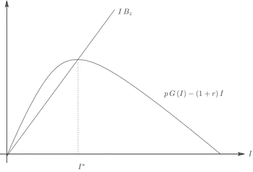
whereI∗ is such thatpG′(I∗) = 1 +r and that the corresponding surplus is positive.10
We characterize equilibrium allocations in terms of the incentive parameter B. As
a starting point, we introduce the threshold value Bz, which defines the lowest level of
incentives compatible with thefirst-best level of investment:
Bz =
pG(I∗)−(1 +r)I∗
I∗. (1)
Figure 1 identifiesBz using the total surplus hump-shaped curve,S =pG(I)−(1+r)I,
and straight lines starting from the origin with slope equal to B. Equation (1) implies
thatBz is the slope of the ray that cuts the surplus’ curve at its maximum.
If B = Bz, then for the first-best investment I∗ to be feasible, the (IC) constraint
must bind. From equation (1) it follows that in every economy whereB =Bz, whenever
I∗ is implemented, the borrower gets the entire surplus. Lenders’ profits are equal to zero
and the corresponding aggregate repayment will beR∗ such that pR∗−(1 +r)I∗ = 0.11
Whenever B > Bz allocations giving zero-profits to the lenders are feasible only if the
level of debt is taken to be lower than I∗.12 We denote ¯I(B) the constrained-maximum
level of aggregate investment compatible with the incentive structureB. It has to be such
that:
pG I¯(B)
−(1 +r) ¯I(B) =BI¯(B),
and ¯I(B) < I∗ holds. Finally, whenever B < Bz, it is possible to achieve I∗ and
to leave some extra-surplus to lenders. One should also notice that for every B < Bz
10
Inada conditions guarantee the existence of such anI∗.
11Of course, this implies that every lender earns zero profit, given that their condition is symmetric and
limited liability holds.
G(I)
I Bz
I I∗
p G(I)−(1 +r)I
Figure 1: Graphical representation ofBz
it would be feasible to implement the first best level of investment I∗ in a monopolistic
environment.
3.1 Characterization
In a scenario where credit relationships take place under the assumption of exclusive
contracting, the borrower can only accept at most one contract at a time. If lenders
compete `a la Bertrand over contracts, at equilibrium the borrower will appropriate the
whole surplus and they will always receive zero profits.13 Notice that competition under
exclusivity delivers the first-best level of credit I∗ only for those economies where the
incentive problems are very mild (B < Bz). If the incentive to shirk is high enough, say
B≥Bz, then zero-profit equilibria will be associated to the constrained amount of credit
¯
I(B).
If we allow for non-exclusive contracting, then we formally enter into a common agency set-up. Given the high degree of externalities involved in the analysis, positive profits equilibria and low levels of aggregate investment will be a typical feature of the analysis. In our model, we can sustain zero-profit equilibria with competition among lenders offering non-exclusive contracts for those parameter values which make the moral hazard problem very mild. As will be clear from the following discussion, equilibria exhibit different
features according to the magnitude of the parameter B relative to the level Bz. To
provide a full description of equilibrium outcomes it is useful to introduce the threshold:
13
The mechanism of undercutting on each opponent’s proposal squeezes any possible rent for the lenders. There cannot be an equilibrium with positive profits for the lenders, given they are all identical and the entrepreneur chooses only one proposal.
Bc =
p G(I∗)−I∗(1 +r)
2I∗ ,
which is lower thatBz and in particular it holds 2Bc =Bz. From the definition ofBc,
we can argue that whenever B < Bc < Bz and there are at least two lenders offering the
zero-profit contract (R∗, I∗), thenI∗ can be sustained also in the presence of two lenders.
In addition, let Bm be the minimal incentive level sufficient to sustain the monopolistic
outcomeIm, where: Im= arg max I πm= arg max I pG(I)−BI−(1 +r)I,
and denoteBl the threshold level of incentive such that:
Bl=
p G(Im)−Im(1 +r)
I∗+I
m
.
Then, for every B < Bl < Bz it is feasible to implement the monopolistic outcome
even if the supplementary amountI∗ was offered.
We are now ready to provide a simple characterization of equilibria in terms of the
incentive parameterB.
Considering those situations where incentive problems are very mild, we can state the following:
Proposition 1 WheneverB ≤Bz, then the outcome (R∗, I∗) can be supported as a (pure
strategy) equilibrium of the gameΓ. In particular:
i) If B ≤Bc, then (R∗, I∗) is an equilibrium outcome for any N.
ii) If B ∈ (Bc, Bz], then there exists a critical number of lenders NB such that for all
N > NB the aggregate allocation (R∗, I∗) is an equilibrium outcome.
iii) For everyB ∈(Bc, Bl], there exists an equilibrium where only one contract is bought.
The contract guarantees positive profits to the unique active lender. Furthermore, there is a second lender who offers a zero-profit contract that is not accepted. All other lenders are not active.
Proof. The proof is given in the Appendix.
The intuition for the result (i) is the following: consider a scenario where (N −2)
lenders are not active, while each of the remaining two can offer a contract associated to a level of debt equal toI∗. Notice that by definition, 2B
c =Bz: this guarantees that two
lenders are enough to sustain the zero-profit equilibrium. If B = Bc, then the borrower
is indifferent between accepting any of the two contracts exerting the desired high effort,
and accepting both of them taking low effort. As long as any single lenderk=i, joffers a
contract different from the zero-profit one Rk6= I
∗(1+r)
p , Ik 6=I
∗, a Bertrand argument
applies: the two-lenders competition generates undercutting on each other’s offer until the marginal cost of funds meets the marginal revenue.
One should note that the competitive result emerging in a scenario of exclusivity can hence be implemented even without imposing exclusivity clauses. If the incentive to shirk
is low, then, despite the high amount of externalities associated to competition under non-exclusivity, the first best outcome can still be reached.
If the incentive to take the low action falls between Bc and Bz, then zero-profits
equilibria may arise only ifN is large enough. This is stated in (ii); in this case, there is no room for a single lender to offer the contract (R∗, I∗) and trigger the low effort choice. The borrower will always have an incentive to accept it in conjunction with other zero profit contracts and shirk. We hence consider a scenario where all lenders offer the contract (Ri, Ii), whereIi= I
∗
N−1 andRi is the repayment level that guarantees zero-profits to the
i-th lender when offering the loan amount NI−∗1, i.e. Ri = I
∗(1+r)
(N−1)p. The borrower accepts
(N −1) offers and selects e=eH. All active lenders enjoy zero profits, but they cannot
have an incentive to deviate given the existence of the inactive one. It is then possible
to find a level of N high enough such that this last lender could not profitably deviate
without inducing low effort.
Finally, (iii) identifies a situation where positive profit may emerge even though the
incentive to take low action is relatively small. In such a case, the first-best level of
investment I∗ will be achieved but the distribution of the total surplus will be rather
favorable to the lenders. The equilibrium is sustained by latent contracts, i.e. contracts which are not bought at equilibrium and are used to deter entry. The analysis of these sort of equilibria has been first introduced by Hellwig (1983) and Arnott & Stiglitz (1993), and then developed by Bisin & Guaitoli (2004).
If we consider the caseB > Bz, then positive profits equilibria are a general feature of
the analysis. Let us first observe that:
Lemma 1 When B > Bz, at every (pure strategy) equilibrium of the game Γ the IC
constraint binds.
Proof. The proof is given in the Appendix.
When the incentive to take the low action is low enough, sayB ≤Bz, then lenders will
effectively compete `a la Bertrand, and the IC constraint will bind at the first best level
I∗. The previous Lemma emphasizes that the existence of a binding incentive constraint
will be a general feature of our economy, independently of the distribution of surplus.14
The following proposition provides a full characterization of equilibria in this region.
Proposition 2 If B ≥Bz, then no allocation guaranteeing zero-profit for lenders can be
sustained at equilibrium. In addition,
iv) If B ∈ [Bz, Bm), there is a critical number of lenders NB such that for every
N ≥NB, there exists a positive profit equilibrium. The equilibrium outcome
NR, N˜ I˜is characterized by the following set of equations:
phGNI˜−NR˜i=phG(N−1) ˜I−(N −1) ˜Ri (2)
phGNI˜−NR˜i=BNI˜ (3)
14
and exhibits the feature that:
(N −1) ˜I > Im (4)
v) If B ≥Bm, then the monopoly outcome can be supported at equilibrium for any N.
Proof. The proof is given in the Appendix.
If the incentive problem is relevant, given the concavity of theG(.) function, then any equiproportional reduction in both the repayment and the credit offered by a single firm
satisfies the IC constraint as a strict inequality. Hence, there is room for a profitable
deviation to break any zero-profit equilibrium.
One should also notice that (iv) refers to an equilibrium where all theNexisting lenders
are active and the borrower is indifferent between accepting (N−1) or N contracts while
exerting high effort, as shown by (2). This no-side-contracting condition is crucial to
establish existence of equilibria with positive profits in several works on moral hazard in
insurance economies because it prevents additional purchases of insurance.15 When the
borrower accepts N contracts, her Incentive Compatibility constraint (3) binds. Finally,
the aggregate level of credit issued by (N −1) lenders is strictly greater than Im that
corresponds to the investment chosen by one monopolistic lender (4). At equilibrium, every lender is active in the market, though the aggregate investment level turns out to be strictly
lower thanI∗. Competition over financial contracts and moral hazard determine rationing
in credit supply and redistribution towards the financial sector. Whenever B > Bz, we
are in the increasing part of the social surplus functionS =p G(I)−(1 +r)I represented
in Fig. 1. As a consequence, a single lenderioffering a zero-profit contract can profitably
deviate if all the others are playing a zero-profit strategy: a Bertrand outcome cannot be sustained.
When the moral hazard problem is very relevant, say B ≥Bm, then any credit level
different from the monopoly one induces shirking, as stated in part (v) of Proposition 2.
The main concern of this paper is to characterize the welfare properties of credit market equilibria when multiple lenders compete over loan contracts. This analysis is developed in the next section.
4
Welfare analysis
We provide here a description of the economy’s feasible set, that is of the set of players’ payoffs corresponding to the allocations implementable by a (benevolent) social planner.
We introduce the notion of social planner and the related concept ofconstrained efficiency
in the same way as it is done in the literature on incentives in competitive markets (see for instance Bisin & Guaitoli (2004)), but we manage to characterize the whole constrained
Pareto frontier. The social planner will choose the aggregate investment level I and the
aggregate repaymentRto maximize his preference relation over the aggregate feasible set
that is usually named theutility possibility set.
We will henceforth denote πL the payoff earned by the lenders in the aggregate credit
sector and πb the corresponding borrower’s payoff. Let us start considering the
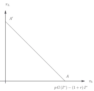
first-best situation, where the relevant constraints faced by the planner are those imposed by technology and resources (together with limited liability requirements). The corresponding utility possibility set is:
F(πL, πb) = (πL, πb)∈R 2 +:πL+πb ≤pG(I∗)−I∗(1 +r) (5) πL πb A A′ p G(I∗)−(1 +r)I∗
Figure 2: The first-best Pareto frontier
The frontier of the set F is referred to as the first-best Pareto frontier. All the arrays
(πL, πb) belonging to this Pareto frontier are such that there does not exist a pair (πL′ , πb′)∈
F with π′L≥πLand π′b> πb or π′L> πL and πb′ ≥πb.
Observe that the payoffs functions πL(R, I) and πb(R, I) evaluated at the high level
of effort are both linear in the aggregate repayment R. As a consequence, the first-best
Pareto frontier will be a downward-sloping 45-degree line. By using the variablepR as a
transfer, we can draw the first-best Pareto frontierπ∗
L(πb∗) as the line depicted in Figure 2.
Every point on the first-best Pareto frontier corresponds to the optimal investment levelI∗. In particular, pointAidentifies a situation where the whole surplus is distributed
to the borrower, π∗
b = pG(I∗)−(1 +r)I∗, so that p R = (1 +r)I∗, i.e. πL∗ = 0. If we
consider the opposite case πb∗ = 0, then from (5) we get pR = pG(I∗), i.e. lenders are
receiving everything and the borrower is left at her reservation utility of zero (pointA′). The second-best allocations are those implementable by a planner who is facing infor-mational as well as feasibility constraints. Theconstrained utility possibility set is the set of outcomes (πL, πb) such that:
F′(πL, πb) =
(πL, πb)∈R 2
+ :πL≤π∗∗L (πb∗∗, B), πb ≤πb∗∗∀πb∗∗∈[0, pG(I∗)−I∗(1 +r)]
where for every givenπ∗∗b ,πL∗∗(π∗∗b , B) is such that:
πL∗∗(πb∗∗, B) = max
R,I pR−(1 +r)I (6)
s.t.
pR−(1 +r)I+πb∗∗≤pG(I)−(1 +r)I (7)
πb∗∗≥BI (8)
With respect to the first-best problem, we have introduced here the Incentive
Compat-ibility requirement appearing in equation (8). Observe that for a given π∗∗
b , the lender’s
objective function is monotone in R, hence equation (7) will bind at the optimum. We
can therefore substitute the expression forpR obtained in (7), in the objective function.
The system (6)-(8) can be rewritten as:
πL∗∗(π∗∗b , B) = max I p G(I)−π ∗∗ b −(1 +r)I (9) s.t. πb∗∗≥BI (10)
One should notice that the constrained utility possibility set and the second-best Pareto
frontier are parameterized to the given incentive structure B. Recall that we defined Bz
as the level of the incentive parameter such that:
pG(I∗)−(1 +r)I∗ =BzI∗
implying thatpR∗ = (1 +r)I∗, i.e. lenders make zero profits. Hence,
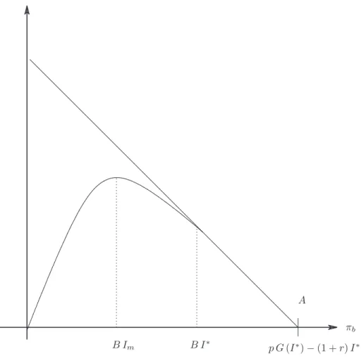
∀B < Bz pG(I∗)−(1 +r)I∗< BI∗
That is, constraint (10) is slack and the first-best is feasible in the second-best problem. In particular, the point (π∗∗
b , πL∗∗) = (pG(I∗)−(1 +r)I∗,0) belongs to the second-best
Pareto frontier (point A in Figure 3). Hence, given that B is strictly lower than Bz,
there is room to reduce π∗∗b without making the constraint (10) binding. There will
therefore be an interval of entrepreneur’s utilities, i.e. π∗∗
b ∈ [BI∗, p G(I∗)−I∗(1 +r)],
such that the second-best Pareto frontier π∗∗
L (π∗∗b , B) coincides with the first-best one
πL∗(πb∗) (Figure 3). By reducing the entrepreneur’s payoff we get to πb∗∗ = BI∗ and
π∗∗
L =p G(I∗)−I∗(1 +r)−BI∗. Every further reduction in π∗∗b will imply a decrease in
B Im p G(I∗)−(1 +r)I∗
A
πb
πL
B I∗
Figure 3: The first and second-best Pareto frontiers forB < Bz
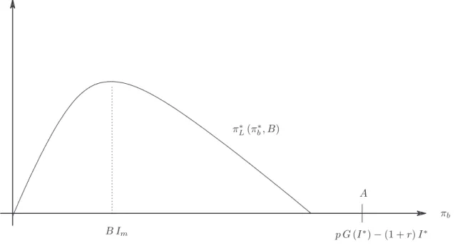
If we consider the case B > Bz, then equation (10) will always be binding at the
optimum level of investment, hence it will not be possible to sustain the first-best
invest-ment level I∗. As a consequence, for every B greater than Bz the second-best frontier
π∗∗
L(π∗∗b , B) will always lie below the first-best one, as it is depicted in Figure 4.
For the cases of relatively mild incentive problem the second-best frontier has therefore a linear part, that corresponds to the implementation of the first-best level of investment (Figure 3); whenever the moral hazard becomes harsher, then the frontier contracts in-wards (Figure 4).
No matter the value ofB, the highest possible payoff for the lending sector corresponds
to the monopolistic allocation, when the entrepreneur is squeezed to a payoff ofπ∗∗
b =BIm
and the lenders appropriate all the rest.16 Whenever π∗∗b < BIm every reduction in πb∗∗
calls for a reduction inπ∗∗
L. In the limit the only way to setπ∗∗b = 0 is to fix an investment
level equal to zero, so that there will not be anything left for the lenders, either. Finally,
we argue that the concavity ofG(I) induces a concavity in the second-best Pareto frontier
(Figure 3 and Figure 4).
16
Recall that every monopolistic investment depends on the value of the incentive parameter, hence it should be writtenIm(B).
πL B Im π∗ L(π∗b, B) πb A p G(I∗)−(1 +r)I∗
Figure 4: The second-best Pareto frontier forB > Bz
Lemma 2 Take any B, for every π∗∗
b ≤BI∗ the frontierπL∗∗(π∗∗b , B) is a concave curve.
In particular,πL∗∗(π∗∗b , B)has a maximum inπb∗∗=BIm. For everyπb∗∗< BIm,πL∗∗(π∗∗b , B)
is monotonically increasing.
Proof. If (10) is not binding, we are back to the linear part of the frontier, which is
trivially concave. The interesting case is that of a binding IC constraint (10). Given πb∗∗
andB, thenI is uniquely determined and given byI = π
∗∗ b B . As a consequence, we get: π∗∗L(π∗∗b , B) =pG π∗∗ b B −π ∗∗ b B (1 +r)−π ∗∗ b
that is a strictly concave function ofπ∗∗b . In particular, forB > Bz the second-best Pareto
frontier is strictly concave.
Defining the constrained Pareto frontier of the economy gives us more intuitions about the welfare implications of competition over loan contracts. The existence of positive profit equilibria and some form of rationing in credit markets, where an arbitrarily large number of homogeneous lenders is competing, turn out to be the by-products of the competitive process under asymmetric information. In such circumstances, we find that a planner facing the same informational constraints as the lenders, cannot implement Pareto-dominant allocations with respect to the equilibrium outcomes of the strategic
interactions between N lenders and a single borrower.
Let us examine the equilibria of the credit market. The equilibria characterized in Proposition 1 involve either a competitive outcome where lenders earn zero-profit (parts
iand ii) or the existence of some latent contracts sustaining positive-profit for the active financier (partiii). It is quite intuitive that the competitive equilibria in i) andii) lie on
the linear part of the frontier, in fact they correspond to pointAin Figure 3. The equilibria with positive profits and latent contracts in iii) fall in the region B < Bz. There, it is
always possible to sustain the first-best level of investment I∗ together with π∗∗
b > BI∗.
The equilibrium level of investment would be the same that a social planner would choose when solving (9)-(10) with a slack incentive compatibility constraint. Hence, the latent contracts are just a device for a different sharing of the surplus among the contractual parties. These equilibrium allocations would correspond to points on the linear part of
the second-best Pareto frontierπ∗∗
L (πb∗∗, B) as depicted in Figure 3.
The equilibria described in Proposition 2 satisfy the same property. Their crucial
feature turns out to be that theIC constraint is satisfied as an equality. As a consequence,
to every payoff earned by the entrepreneur/borrower will correspond the same level of credit issuance, both at equilibrium and at the optimum. As a consequence, the payoff
earned by the lending sector will also be the same:17
Proposition 3 ConsiderB≤Bz, all equilibria defined in Proposition 1 are efficient, and
the optimal level of investment I∗ is implemented.
Take a B > Bz and consider the allocations of the positive-profits equilibria defined in
Proposition 2, they all belong to the constrained Pareto frontierπ∗∗
L (πb∗∗, B). Proof. The proof is given in the Appendix.
The main result can hence be summarized as follows: the common agency interactions in the market for loans deliver constrained Pareto efficient equilibria, despite the external-ities due to strategic competition over financial contracts. The next section investigates in detail the sources of this finding.
5
Discussion and conclusions
We proposed a simple characterization of the constrained Pareto frontier. At the
opti-mum, either the first best outcome is implemented, or the Incentive Compatibility (IC)
constraint binds as an equality.
The equilibrium outcomes described in Proposition 1 are such that the investment level
I∗is achieved, whereas those characterized in Proposition 2 imply a bindingICconstraint.
This is the key to understand the efficiency result: whenever theICconstraint binds, there
is a one-to-one relationship between the entrepreneur’s payoff and the amount of credit issued at equilibrium (and at the optimum). This determines aggregate loan supply, and hence the social surplus. The overall payoff for lenders is determined residually. In particular, the no-side-contracting condition (4) only serves as a redistributive rule within the lending sector.
In our context, whenever theIC constraint is not binding, there is always room for an
additional lender to offer a profitable contract that will be accepted without inducing the borrower to switch to the low effort.
17See Proposition 6 in the Appendix for the generalization of this result to the case of a non-linearB(I)
This intuition provides useful insights for further discussion on the literature on com-petitive markets under asymmetric information. In particular, we can relate our findings to the studies on competition in insurance and financial markets: Arnott & Stiglitz (1993), Hellwig (1983), Bizer & DeMarzo (1992), Kahn & Mookherjee (1998), Bisin & Guaitoli (2004) among others. These researches emphasized how asymmetric information in non-exclusive markets may give rise to the so-called ”non-price equilibria”, that typically fail to be (constrained) Pareto efficient. If one modifies the basic description of the economy so to get a binding Incentive Compatibility constraint at equilibrium, then efficiency can be reestablished.
Take as an example the recent work of Bisin & Guaitoli (2004), where the inefficient equilibria are those supported by latent policies. In their framework, as in all the liter-ature dealing with insurance problems, the agent is typically risk-averse with respect to the event of an accident. Introducing a risk-neutral agent eliminates the extra-premium for misbehaving, hence it reduces the (endogenous) reservation utility of the low effort
at equilibrium and leads to a binding IC constraint. It is then possible to verify that
all the equilibria of their insurance model have the same efficiency properties, i.e. they
induce second-best efficient outcomes.18 Hence, introducing risk neutrality is a means
to recover a binding IC constraint. Even though risk aversion is a natural assumption
in insurance set-ups, most of the banking literature typically considers risk-neutral
en-trepreneurs/borrowers.19
Our investigation, then, contributes to improve the understanding of the welfare prop-erties of strategic competition among intermediaries in the presence of a single agent. Intuition seems to suggest that whenever common agency games with complete informa-tion are considered, then efficient outcomes can be supported at equilibrium as long as
theIC constraint binds.20 The effect of externalities from competition pass through the
incentive structure, hence if it was sensitive and reactive enough, we could identify the effects of competition on contracts. A related research along this line explores the possi-bility to enrich the contractual mechanism so to have several dimensions to measure the competition. It is shown that if the financial contracts includes some monitoring activ-ity, together with loan amount and repayment, then the constrained inefficiency result
emerges.21 Having a richer contractual mechanism is another way to sustain non-binding
Incentive Compatibility constraint.
Finally, it is important to remark that our analysis is focused on the simple scenario where lenders’ strategies are restricted to be take-it-or-leave-it offers. Investigating the welfare implications of competition through more complex mechanisms is still a very open
18
With reference to Bisin & Guaitoli (2004), if a risk-neutral agent is considered, then their equation (7) coincides with ourI Cconstraint. In addition, examining equations (8)−(12) which they use to define
the planner’s problem, one can check that theI Cbinds also at the optimum and that the second best can
be decentralized.
19For a detailed analysis of the role of risk-aversion in principal-agent models of the credit market see
Freixas & Rochet (1997).
20Importantly, we have not restricted in any way participation decisions. That is, our results apply to
the so-called ”delegated” scenario, as well.
21
problem. This is a relevant issue for policy matters and will be a major topic for future research.
6
Acknowledgment
The inspiration for the work came from the paper that Uday Rajan and Christine Parlour published on AER in december 2001. This is now part of a research project started with U. Rajan when we were all together at CORE.
We thank K. Dam, C. d’Aspremont, M. Franchi, P. Gottardi, D. Guaitoli, E. Minelli, D. Perez-Castrillo for helpful discussions and comments. We also thank the participants to seminars at CORE, Financial Market workshop at IDEI (Toulouse) and to the PAI workshop in Gent. All responsibility remains to the authors
7
Appendix
To show that our results are robust to the introduction of more general preference struc-tures for the entrepreneur, in the proofs we will consider the situation in which the
en-trepreneur’s private benefit is represented by the non-linear function B(I), whose
prop-erties have been stated in Section 2. The specification B(I) =BI makes the discussion
clearer in the paper and turns out to be unrestrictive.
From now on, we consider a total private benefit function B(I) that is continuous,
increasing and convex in I:
B(0) = 0, B′(I)>0, B′′(I)≥0,
and such that the Inada conditions hold: lim
I→0B
′(I) = 0, and lim
I→∞B
′(I) = +∞.
Everything else remaining unchanged, we now characterize the equilibrium allocations in terms of the incentive functionB(.). More precisely, we introduce the setsBz,Bc and
Bl corresponding to the parametersBz,Bc and Bl considered in the text.
Definition 2 We take Bz to be the set of functions B(.) such that:
B(I∗)≤pG(I∗)−(1 +r)I∗; (A.1)
Bc to be the set of functions B(.) satisfying:
B(2I∗)≤p G(I∗)−(1 +r)I∗; (A.2)
and finally, we refer to the set Bl as to the set ofB(.) such that:
B(I∗+Im)≤pG(Im)−(1 +r)Im. (A.3)
Under our assumptions onB(.), it holds that if B(.)∈ Bc then B(.)∈ Bz and B(.)∈ Bl;
in addition, it is also true thatB(.)∈ Bl impliesB(.)∈ Bz.
We now restate the propositions included in the text as relative to the sets of functions
B(.).
Proposition 4 WheneverB /∈ Bz, then the outcome (R∗, I∗) can be supported as a (pure
strategy) equilibrium of the gameΓ. In particular,
i) Take any B(.)∈ Bc, then (R∗, I∗) is an equilibrium outcome for any given N;
ii) If B(.)∈ Bz, andB(.)∈ B/ c then there exists a critical number of lenders N¯B s.t. for
allN >N¯B the aggregate allocation (R∗, I∗) is an equilibrium outcome;
iii) For every B(.)∈ Bl, there exists an equilibrium where only one contract (say, Ci) is
bought. The contract guarantees positive profits to lender i. Furthermore, there is a second lender (say, lender j) who offers a zero-profit contract that is not accepted. All other lenders are not active.
Proof of part i). We consider the following array of offered contracts:
{(Ri, Ii) = (Rj, Ij) = (R∗, I∗) fori6=j; (Rk, Ik) = (0,0) ∀ k6=i, j}.
That is, there are two lenders, say lenderiand lenderjwho offer the first-best allocation,
while all other lenders are offering the null contract (0,0). The borrower is indifferent
between accepting thei−th and the j−th contract; given that B(.)∈ Bc, accepting all
contracts and choosing low action is never a best reply.
In such a scenario, no lender has a profitable deviation given that the first-best outcome is implemented and the borrower’s profit is maximized.
Proof of part ii). Consider the case of B(.)∈ Bz and B(.)∈ B/ c. If every lender offers
the contract (R′, I′) = R∗
N−1,
I∗
N−1
, it is incentive compatible for the borrower to accept
(N−1) out of N contracts, provided that the high effort is chosen.
By doing so, the first-best aggregate level of investment would be implemented; the bor-rower would achieve her maximum expected payoff with each single lender getting zero profits. Let us evaluate if there exist profitable deviations for lenders.
Given what his opponents offer, lenderi can never propose a loan that the borrower will
accept and guarantees him positive profits. When allj6=ilenders offer (R′, I′), whatever
lenderiproposes, the borrower can always buy the remaining (N−1) contracts and achieve
her maximum payoff. Hence, it is a best response for lender i to offer (R′, I′) when all
other lenders offer (R′, I′).
Finally, to guarantee that the entrepreneur has no profitable deviations, we have to take into account the incentive to buy all available contracts and shirk:
pG N−1 N−1I ∗ −(N−1)I ∗(1 +r) N −1 ≥B I∗ N N −1 ; (A.4)
that is, we want that the utility she gets from buying all N contracts and exerting low
action be lower than the first-best payoff:
pG(I∗)−I∗(1 +r)≥B I∗ N N −1 . (A.5)
As the functionB(.) belongs to the setBz, then it satisfies the condition:
pG(I∗)−I∗(1 +r)≥B(I∗). (A.6)
Thus, if N is high enough, condition (A.5) is satisfied. Hence, for every B(.) ∈ Bz and
B(.) ∈ B/ c and N high enough, the borrower has no incentive to deviate from buying
(N −1) contracts and choosing high effort. There does not exist any contract for any
lenderi that gives him positive profits and is accepted by the borrower. Hence, (R′, I′)
for each lender, and the borrower accepting (N −1) contracts and exerting high effort
constitute an equilibrium.
Proof of part iii). Take any B(.)∈ Bl and consider the functionx(I) =pG(I)−I(1 +
The equilibrium is defined by:
one lender, say lender i, offering the contract Ci = (Ii, Ri) with Ii = I
∗ and R
i s.t.
pRi=pG(I∗)−I∗(1 +r)−(pG(I′)−I′(1 +r)), hence making positive profits;
a second lender, say lender j, offering the zero-profit contract Cj = (Ij, Rj) such that
Ij =I′ andpRj = (1 +r)I′;
all other lenders k ∈ N and k 6= i, j offering the null contract Ck = (0,0) and the
borrower acceptingCi, only.
Given the behavior of the other players, lenderimust offer the borrower at least a payoff
of pG(I′)−I′(1 +r) in order for his contract to be bought. Hence, he has the incentive
to set the investment level atI∗ so to realize the maximum amount of profits p R
i.
Let us now consider lender j: he cannot profitably deviate from the level of investment
Ij = I′ and be guaranteed that his offer is accepted, without inducing the borrower to
shirk to the low action.
Given the existence of the latent contract j, no contract offering positive investment level
proposed by any of the inactive lenders will be accepted at equilibrium.
Finally, the borrower is indifferent between accepting either contract i or j in isolation
and choosing high effort, and buying both contracts and choosing low action. That is, acceptingionly is a best reply.
To complete the characterization of all relevant equilibria, we need to define the set of
incentive functions related to the implementation of the monopolistic outcome, i.e. Bm.
Definition 3 We refer to Bm as to the set of functions B(.) such that:
BIm+I ′′ ≤pGI′′−(1 +r)I′′ (A.7) where I′′ =argmax I pG(I)−(1 +r)I−B(Im+I).
Lemma 3 When B(.) ∈ B/ z, at every (pure strategy) equilibrium of the game Γ the IC
constraint binds.
Proof. We have to show that there cannot be an equilibrium with:
p " G X i∈A Ii ! − X i∈A Ri !# > B X i∈N Ii ! , (A.8)
whereAis the set of accepted contracts.
Notice that equation (A.8) implies that for any given B(.), the aggregate investment is
X
i∈A
Ii < Im = arg max I∈R+
p G(I)−(1 +r)I−B(I). (A.9)
In addition, the argument is not restricting equilibria to be symmetric.
First, take the caseA(N. At the candidate equilibrium there are contracts that are not
accepted, hence lenders earning zero profits. Let the contract offered by lenderj be one
of those, i.e. j /∈ A.
Now, assume lenderj deviates, offering Cj = (Rj, Ij), where the deviation is such that:
lenderj makes positive profits;
the borrower performs the desired level of effort,
the borrower accepts the new contract together with the contracts contained inA.
In formal terms, the deviation is such that:
p " G X i∈A Ii+Ij ! − X i∈A Ri+Rj !# > p " G X i∈A Ii ! − X i∈A Ri !# , πj =pRj−(1 +r)Ij >0. (A.11)
We can therefore derive the following expression forpRj:
0< pRj < p " G X i∈A Ii+Ij ! −G X i∈A Ii !# . (A.12)
Now, let us remark that the following inequality
p " G X i∈A Ii+Ij ! −G X i∈A Ii !# −(1 +r)Ij >0. (A.13) is satisfied whenever: pG′ X i∈A Ii ! >(1 +r), (A.14)
which is always true as long as P
i∈AIi < Im and Ij “small enough”. It implies that it
exist a repayment Rj close enough to pG Pi∈AIi+Ij
−pG P
i∈AIi
such that (11) and (11) are satisfied.
If the new offer of lenderjwas such to induce modification in the set of accepted contracts
as long as equation (A.8) holds, there always exists a profitable deviation for lenderj. For a deviation to be profitable, it must now be:
p " G X i∈A′ Ii+Ij ! − X i∈A′ Ri+Rj !# > p " G X i∈A Ii ! − X i∈A Ri !# , πj =pRj−(1 +r)Ij >0,
whereA′ is the new set of accepted contracts. By construction: p " G X i∈A′ Ii+Ij ! − X i∈A′ Ri+Rj !# ≥p " G X i∈A Ii+Ij ! − X i∈A Ri+Rj !# .
Finally, asRj andIj are “small”, the set of accepted contract A′ cannot be the empty set.
Now, consider the case A=N, and let (Ii, Ri)i∈N be the collection of non-null contracts
offered at equilibrium. Clearly, if any of the lenders was offering the null contract, i.e.
Ck = (0,0) for some k∈N, then the previous argument for a profitable deviation would
apply. If p " G X i∈N Ii ! − X i∈N Ri !# > B N X i=1 Ii ! (A.17)
then any of theN lenders would have a profitable deviation: he could raise the repayment
of his contract until (A.17) binds.
Proposition 5 If B(.) ∈ B/ z, then no allocation guaranteeing zero profits to the lenders
can be sustained at equilibrium. In addition,
iv) If B(.) ∈ Bm, then there is a critical number of lenders NB such that for every
N ≥NB, there exists a positive profit equilibrium. The equilibrium outcome
NR, N˜ I˜is characterized by the following set of equations:
phGNI˜−NR˜i=phG(N −1) ˜I−(N −1) ˜Ri (A.18)
phGNI˜−NR˜i=BNI˜ (A.19)
and exhibits the feature that:
(N −1) ˜I > Im (A.20)
v) If B(.) ∈ B/ m, then the monopoly outcome can be supported at equilibrium for any
givenN.
Proof. Assume by contradiction that B(.) ∈ B/ z and that there exists a zero-profit
equilibrium. At equilibrium, it should beP
i
Ii≤I¯(B), otherwise the borrower will strictly
prefer to accept all loans and shirk.22 Now, there must be at least two lenders offering a
positive loan amount, otherwise monopoly would be implemented breaking the conjectured zero-profit equilibrium. Let us call these lendersiand j and let Ii >0 and Ij >0 be the
respective amount of loan each of them offers.
22
Paralleling the discussion in the text, we take ¯I(B) to be the credit level that guarantees the full appropriation of surplus by the borrower, given the incentive structureB.
It must be that: ¯I−Ij ≥Ii >0, and since we conjectured a zero-profit equilibrium with
two strictly positive contractual offers: pG(Ij)−(1 +r)Ij > B(Ij).
Hence, there should exist anǫ >0 such that:
pG(Ij+ǫ)−(1 +r)(Ij+ǫ)> B(Ij+ǫ)
Given we are in the increasing part of the surplus function,
pG(Ij+ǫ)−(1 +r)(Ij+ǫ)> pG(Ij) + (1 +r)Ij.
But then, there exists a δ >0 such that:
pG(Ij+ǫ)−(1 +r)(Ij+ǫ)−δ >max{pG(Ij) + (1 +r)Ij, B(Ij+ǫ)}.
That is, there exists a profitable deviation for lenderiwhen offering (ǫ, δ).
Proof of part iv). The proof is organized in two steps. First, we show that there is an aggregate contractNR, N˜ I˜which is a solution of the system (A.18)-(A.19) and satisfies (A.20). In a next step we show that the strategy profile (Ri, Ii) =
˜
R,I˜for every lender
i∈N together with the borrower decision of accepting all contracts and choosing the high
level effort is a subgame perfect equilibrium. Considering (A.8) and (A.9) together we get:
p G(N−1) ˜I− 1− 1 N GNI˜ − BNI˜ N = 0. (A.21) We definef(I) =p G((N−1)I)− 1−N1 G(N I) −B(NN I).
Notice that the aggregate investment level belongs to the interval
Im,I¯(B)
, where ¯I(B) is the level of investment such that
pG I¯(B)
−B I¯(B)
−(1 +r) ¯I(B) = 0
andImrepresents the monopolistic level of investment corresponding to the relevantB(.)∈
Bm. It is easy to check that ¯I(B)> Im. Now, let us denote ¯I(B)o=
¯ I(B) N . Evaluating the functionf(I) at ¯I(B)o, we obtain: f I¯(B)o =pG (N −1) N I¯(B) −pG I¯(B) +1 +r N I¯(B). (A.22)
Given that the function G(.) is concave and recalling that pG′ I¯(B)
> 1 +r, we have that: pG( ¯I(B))−(1 +r) N I¯(B)> p G (N−1) ¯I(B) N (A.23) andf I¯(B)o <0.
Using a similar argument, and recalling the definition of Bm we can check that for every
f Im N −1 >0. (A.24)
By continuity off(.), for everyN ≥NB there exists a value ˜I(B, N) such thatf
˜
I= 0.
Given ˜I, the value of R satisfying (A.18)-(A.19) can hence be defined in a direct way.
Now, we have to show that at equilibrium every lender will offer the contract R,˜ I˜and
that the borrower will always have an incentive to accept all contracts and to select the high action.
Let us start with the borrower’s behavior: if each lender is playing ( ˜R,I˜), then the
bor-rower’s strategy of acceptingN contracts and exerting high effort is a best reply. Equations
(A.18) and (A.19) guarantee that when NR, N˜ I˜ is offered in the aggregate, then the
borrower cannot deviate by accepting (N −1) contracts. No reductions in the number of
accepted contracts will be profitable.
Let us consider now the behavior of the lenders. Suppose all (N−1) lenders except lender
i offer R,˜ I˜ and consider lender i’s best response. Assume lender i offers (Ri, Ii), his
best payoff can be measured with respect to the aggregate amount of loans the borrower takes up: πi =pRi−(1 +r)Ii = =pGkI˜+Ii −(1 +r)Ii−kpR˜ −maxnpG(N −1) ˜I−p(N −1) ˜R, B(N−1) ˜I+Ii o , (A.25)
where πi is lender i’s payoff as a function of (Ri, Ii) and k = {0,1,2, ..., N −1} is the
number of contracts the borrower buys together with the i-th. On the right hand side
of equation (A.25) we represented the surplus at the aggregate amount of investment
kI˜+Ii
net of the reimbursements of theklenders offeringR,˜ I˜and of the borrower’s utility. The borrower’s payoff cannot fall below the minimum between the amount she
obtains accepting the (N −1) contracts and exerting high effort, i.e. pG(N −1) ˜I−
p(N −1) ˜R, and the utility from shirking, i.e. B(N −1) ˜I+Ii
.
We remark that using equations (A.18) and (A.19), the repayment of each of the (N−1)
lenders is given by:
pR˜ =phGNI˜−G(N−1) ˜Ii. (A.26)
Now, let us examine the choice ofIi by the i-th principal.
There can be two cases: eitherIi ≤I˜orIi >I˜.
In the first case, from the definition of the equilibrium the borrower will have to be guaranteed at least pG(N −1) ˜I−p(N −1) ˜R that is greater then B(N −1) ˜I+Ii
for everyIi ≤I˜.
In addition, given Ii≤I˜and the concavity ofG(.), the borrower will buy all the (N −1)
contracts together with thei-th. When choosingIi the lender anticipates how his proposal
affects the entrepreneur’s choice on the number of contracts k she purchases from the
in k up to k =N −1. Take the entrepreneur’s payoff in the case she buys kI˜+Ii and
compare it with buying (N −1) ˜I +Ii, it’s easy to see that: ∀k= 0,1, ..., N −2
pG(N −1) ˜I+Ii −p(N −1) ˜R−pRi> pG kI˜+Ii −pkR˜−pRi (A.27)
Hence, the borrower tries to implement an aggregate loan amount of (N −1) ˜I or NI˜.
This remains true even in the case whenIi>I˜. If lender ichooses to offerIi>I˜and the
number of lenders N is sufficiently high, the concavity ofG(.) implies that the borrower
selects the number of accepted contracts k from the non-deviating lenders according to
the following condition:
pG′kI˜+Ii ≈ pG(NI˜)−pG((N −1) ˜I) ˜ I ≈pG ′(N −1) ˜I (A.28)
Any increase inIimust hence be accompanied by a reduction ink. Conditional on choosing
high effort, the previous discussion completely characterizes the borrower’s choice ofk, i.e.
her best reply in terms of the number of accepted contracts.23
We remark that wheneverIi>I˜, implementing high effort and choosing the associatedk
contracts together withIi is always dominated by accepting all offers and shirking. That
is, for everyIi >I˜we have:
B(N −1) ˜I+Ii
> pGkI˜+Ii
−pRi−kpR˜ (A.29)
To show that the inequality (A.29) holds for every possible choice of Ii, consider that
the i-th lender must earn at least what he could earn offering the contract ( ˜I,R˜), i.e.
pRi−(1 +r)Ii ≥pR˜−(1 +r) ˜I. Let us take the most favorable case for the borrower, that
ispRi−(1 +r)Ii =pR˜−(1 +r) ˜I. In addition, according to equation (A.28), the choice
ofk satisfieskI˜= (N−1) ˜I−Ii. We can therefore rewrite the inequality (A.29) as:
B(N−1) ˜I+Ii > pG(N−1) ˜I−pRi− (N −1)−Ii ˜ I pR˜ (A.30)
Since the equilibrium conditions guarantee: BNI˜ = pG(N −1) ˜I−(N −1)pR˜,
equation (A.30) can hence be rewritten as:
B(N−1) ˜I+Ii −BNI˜>−pR˜−(1 +r)(Ii−I˜) +pR˜ Ii ˜ I (A.31) which becomes: B((N−1) ˜I+Ii)−B(NI˜) Ii−I˜ (Ii−I˜)> pG(NI˜)−pG((N−1) ˜I) ˜ I −(1 +r) ! (Ii−I˜) 23
Notice that wheneverIi>I˜the best reply of the borrower is multivalued. She is indifferent between
buying the i-th contract together with k < N −1 non-deviating ones, and rejecting the offer Ii and
and, considering derivatives, we get:
B′NI˜+ (1 +r)> pG′(NI˜). (A.32)
For everyIi >I˜equation (A.32) is true, since (N −1) ˜I > Im. Therefore, whenever the
i-th lender tries to offer a higher amount of loans Ii >I˜he cannot prevent shirking.
None of the lenders can profitably deviate from the offer ( ˜I,R˜).
Proof of part v). We want to prove that, at equilibrium, there is one lender, say lender
i, offering Ci = (Im, Rm) while the remaining N−1 lenders are offering (0,0). For lender
i,Ci is clearly a best response, since he attains the maximum available profit.
Let us consider if there exist profitable deviations for any of the non-activeN−1 lenders,
say lender j. To have a profitable deviation, lender j should be able to offer some
pos-itive amount of loan Ij > 0 and having his contract accepted either together with the
incumbent’s loan Im or in competition with him.
IfIj is bought together withIm, then the profit the deviating lender could get is given by:
πj =pG(Im+Ij)−(1 +r)Ij−pRm−B(Im+Ij), (A.33)
wherepRm =pG(Im)−B(Im) from the maximization problem of a monopolist. We can
rewrite equation (A.33) as:
πj =pG(Im+Ij)−pG(Im)−(1 +r)Ij−[B(Im+Ij)−B(Im)]. (A.34)
The concavity of G(.) and the convexity of B(.) imply that:
πj < pG′(Im)Ij−(1 +r)Ij−B(Im+Ij) +B(Im)
< pG′(Im)Ij−(1 +r)Ij−B′(Im)Ij
= 0
Hence, lenderj cannot profitably offer a loan that is taken up together with thei-th and
gives him positive profits. In case lenderj tries to compete with the incumbent, the best
he can earn is given by:
πj =pG(Ij)−(1 +r)Ij−B(Im+Ij). (A.35)
Now, the best lenderj can do is to offer the amount of investment that solves: pG′(I
j) =
(1 +r) +B′(Im+Ij). But, given thatB(.)∈ B/ m, by doing so the entrepreneur will always
strictly prefer to buy both contracts and shirk. As a consequence, lenderj does not have
any profitable deviation from offering (0,0).
Let us move now to the welfare properties of market equilibria. The features of constrained Pareto optimal allocations derived in Section 4 naturally extend to a scenario where private
benefits are a non-linear function of the borrowed amountI. First, it is possible to show
that the convexity of theB(I) function preserves the concavity of the Pareto frontier:
Lemma 4 For everyπ∗∗
b ≤B(I∗)the second-best Pareto frontierπL∗∗(π∗∗b , B)is a concave
curve. In particular,π∗∗
L(πb∗∗, B)has a maximum inπb∗∗=B(Im). For everyπb∗∗< B(Im),
π∗∗
L (πb∗∗, B) is monotonically increasing. Proof. If π∗∗
b ≤ B(I∗) is not binding, we are back to the linear part of the frontier,
which is trivially concave. The interesting case is that of a binding incentive compatibility constraint, i.e. πb∗∗=B(I∗). Given πb∗∗ and B, then I is uniquely determined and given byI =B−1(π∗∗
b ). As a consequence, we get:
πL∗∗(π∗∗b ) =pG B−1(π∗∗b )
−(1 +r)B−1(πb∗∗)−πb∗∗ (A.36)
Let us compute the first and second order derivatives with respect toπ∗∗
B: ∂π∗∗ L ∂π∗∗ b =pG′ B−1(π∗∗b ) B−1′(π∗∗b )−(1 +r)B−1′(π∗∗b )−1 ∂2π∗∗ L ∂ π∗∗ b 2 =pG ′′ B−1(π∗∗ b ) B−1′(πb∗∗)2 +pG′ B−1(πb∗∗) B−1′′(π∗∗b )−(1+r)B−1′′(πb∗∗)
SinceB′′≥0, we haveB−1′′≤0 and we can conclude that ∂2π∗∗L
∂ π∗∗ b 2 ≤0. Hence,π ∗∗ L (πb∗∗) is a concave function ofπ∗∗ b .
Eventually, we argue that the equilibrium outcomes characterized through Proposition 4 and Proposition 5 identify (constrained) efficient allocations. Importantly, all these
equilibria are such that the relevant (IC) constraint turns out to be binding. One can in
fact show the following:
Proposition 6 All the (pure strategies) equilibrium outcomes defined in Proposition 4 and Proposition 5 are constrained Pareto efficient. That is, they belong to the frontier
π∗∗
L (πb∗∗, B).
Proof. Let us start with Proposition 4.
The equilibria characterized in parts i) and ii) are competitive equilibria, where lenders
earn zero-profit and the entrepreneur appropriates all the surplus. In addition the
aggre-gate amount of investment is the first-best one,I∗. Hence, they correspond to pointA in
Figure 3 in the text. These equilibria belong to the linear part of the second-best frontier, in fact they are also first-best equilibria.
In part iii) of Proposition 4 we characterize equilibria with latent contracts in the region
B∈ Bz. These equilibria guarantee positive profits to the active lender and zero-profit to