Endogenous Credit Cycles
Chao Gu
Randall Wright
October 12, 2010
Abstract
We study models of credit with limited commitment, which implies endogenous bor-rowing constraints. We show that there are multiple stationary equilibria, as well as nonstationary equilibria, including some that display deterministic cyclic and chaotic dynamics. There are also stochastic (sunspot) equilibria, in which credit conditions change randomly over time, even though fundamentals are deterministic and station-ary. We show this can occur when the terms of trade are determined by Walrasian pricing or by Nash bargaining. The results illustrate how it is possible to generate equi-libria with credit cycles (crunches, freezes, crises) in theory, and as recently observed in actual economies.
JEL classi cation: E2
Key words: credit, commitment, dynamics, cycles
Gu: Corresponding author. 118 Professional Building, Department of Economics, University of Missouri, Columbia, MO 65211. Email: [email protected]. Tel: (573) 882-8884. Fax: (573) 882-2697. Wright: University of Wisconsin and Federal Reserve Bank of Minneapolis. We thank Noah Williams and Christian Hellwig for comments and conversations, as well as the Federal Reserve Bank of Minneapolis and the NSF for research support. Wright also thanks the Ray Zemon Chair in Liquid Assets at the Wisconsin School of Business.
“As we have seen, all Þnancial institutions are at the mercy of our innate
in-clination to veer from euphoria to despondency.” Niall Ferguson, The Ascent of
Money.
1
Introduction
Without doubt, recent events have put credit markets front and center in economics and
Þnance. As Akerlof and Shiller (2009) put it, “the overwhelming threat to the current
economy is the credit crunch.” In the Wall Street Journal (January 27, 2009) Shiller goes
on to say: “To a great extent these traders borrowed short term at low interest rates against collateral of asset-backed securities, of which residential mortgage-backed securities would be just one example. What enabled them to do that? It was the animal spirits. Those
who loaned short to the shadow banking sector were conÞdent. They thought they would
be repaid...They were trusting. But as soon as these lenders lost their conÞdence they were
no longer trusting. It was like a classic bank run, but this time not on the formal banking sector.” Are credit markets susceptible to animal spirits, or extrinsic uncertainty, and why?
There is much work onßuctuations in credit markets driven by the fundamentals, by which
we mean preferences, technologies and policies (see e.g. Kiyotaki and Moore 1997, or the survey by Gertler and Kiyotaki 2010). The goal here is to construct a model in which movements in credit markets are driven by beliefs, not fundamentals. And we want a theory based on explicit microeconomic foundations — not just a story.
Obviously such a theory will have to contain frictions of one form or another, since
frictionless models like Arrow-Debreu, where theÞrst welfare theorem says that equilibria are
e!cient, cannot generate endogenous (self-fulÞlling)ßuctuations in credit conditions.1 While
our model allows for several frictions, including imperfections in monitoring and collateral, we take a stand on limited commitment being the key to understanding credit markets.
1To be more precise, if not pedantic, one might add the adjectives Þnite-dimensional and convex to
Limited commitment naturally leads to endogenous borrowing limits, which may or may not be binding, in equilibrium. We prove that, if one sets up the model carefully, there can be
multiple steady state equilibria with di"erent credit limits and di"erent allocations, as well
as dynamic equilibria where credit limits and allocations vary over time even if fundamentals do not. These exotic dynamics include deterministic cyclic and chaotic equilibria, as well as stochastic equilibria, in which credit conditions change randomly over time even though fundamentals are deterministic and time invariant. In these equilibria, credit conditions change for no reason other than beliefs. We think these results are instructive about credit cycles, crunches, freezes, crises, or whatever one likes to call them in actual economies; they are certainly instructive about what can happen in economic theory.
The model contains inÞnitely-lived agents, where di"erent types may want to borrow
or lend at di"erent points in time. Limited commitment means they are free to renege on
debts whenever they like. Hence we need some way to punish those who behave badly, or reward those who behave well. As is standard, if agents are caught deviating (not honoring their obligations) they are punished by exclusion from access to future credit, but we allow deviators to be caught only probabilistically (imperfect monitoring). In our environment,
collateral mitigates the commitment problem but may not completely solve it. Di"erent
mechanisms are considered for determining the terms of trade. We show how to gener-ate endogenous credit market dynamics using Walrasian price taking and generalized Nash bargaining, and show that this is not possible using some other mechanisms, including
pro-portional bargaining or take-it-or-leave-it o"ers. When endogenous dynamics do arise, the
economic forces di"erent under Nash bargaining and Walrasian pricing: in the former case,
results hinge on the property of Nash bargaining that agents’ individual payo"s need not
increase monotonically as the bargaining set expands; in the latter case, they hinge on the
fact that payo"s in Walrasian markets need not increase monotonically as we relax quantity
There is a large literature on limited commitment and endogenous borrowing constraints.2
These papers typically consider only Walrasian pricing and do not incorporate the frictions considered here, other than limits to commitment (also much of that literature uses pure exchange, while we have production, but this is a detail). Generally, at least some version
of the welfare theorems hold in those models, and they cannot generate ßuctuations except
through changes in fundamentals. We deliver genuinely endogenous ßuctuations. This is
similar to the literature on dynamics in monetary economies.3 Once we reduce our model to
a dynamical system, the techniques used to study it are similar to those in monetary theory,
which is Þne since our objective is to develop an economic model, not mathematical tools.
One thing we learn from this is that credit models with limited commitment behave in some ways like monetary models — they can have complicated sets of equilibrium, including some
displaying exotic dynamics.4 In any case, we think the framework has some nice features:
it is tractable, yet it generates a variety of interesting outcomes. Moreover, by contrast with other models, endogenous dynamics arise here for very reasonable parameters values, including those measuring risk aversion and discounting.
The presentation is organized as follows. Section 2 lays out the environment. Section 3
deÞnes equilibrium. Section 4 analyzes stationary equilibria. Section 5 analyzes dynamics,
including cyclic, chaotic and stochastic equilibria. Section 6 discusses the economics behind the results. Section 7 concludes. All proofs are relegated to an Appendix.
2
Environment
Time is discrete and continues forever. Each period is divided into two subperiods. There
are two types of agents of equal measure in the economy: type 1 agents consume good 1
2Our set up is close to Kehoe and Levine (1993,2001) and especially Alvarez and Jermann (2000). See
also Azariadis and Kass (2007,2008), Lorenzoni (2008), and Hellwig and Lorrenzoni (2009).
3We refer readers to Azariadis (1993) for a textbook treatment and references to the original contributions.
4Sanchez and Williamson (2010) also highlight the relation between credit and money. There are too
and produce good 2; type 2 agents consume good 2 and produce good 1. Both goods are
produced in theÞrst subperiod, but while good1 is consumed in theÞrst subperiod, good2
is consumed in the second. Type2 thus produce before they consume while type1 consume
before they produce. Moreover, only the producer of good 2 can store or invest it across
subperiods. This generates a natural if stylized role for collateralized debt: type 1 gets to
consume in the Þrst subperiod in exchange for a promise to deliver goods in the second
subperiod out the returns on his investments. When the time to deliver rolls around, type
1 has less of an incentive to renege on his obligation than if he had to produce on the spot,
since the cost is sunk. However, so that collateral does not work too well, we assume type 1 can liquidate his investments, by consuming the proceeds himself, say, so that there is an
opportunity cost if not a production cost to making good on one’s promises.5
Agents of di"erent types meet in the Þrst subperiod, and can enter into credit contracts,
described as follows. Suppose in theÞrst subperiod type2produces!for type1to consume,
while type 1produces ", invests it, and delivers the proceeds, say#"$ for type 2to consume
in the second subperiod. The utility from this exchange is%1(!$ ")for type1and%2(#"$ !)
for type2. It should be clear that we can reduce notation by normalizing#= 1, with no loss
in generality. Both utility functions are strictly increasing in consumption and decreasing in
production, strictly concave, twice di"erentiable, and %!(0$0) = 0. We also assume normal
goods for some results.6 Once!is produced, type2has no reason not to hand it over to type
1 in the Þrst subperiod. But in the second subperiod, type 1 can liquidate (consume) the
output" from the previous subperiod, for a payo"of&" over and above the utility from the
original consumption of ! and production of ". The parameter & measures the temptation
5This captures the idea that, as Ferguson (2008) puts it, “Collateral is, after all, only good if a creditor
can get his hands on it.” Also, note that technology does not let type2store or otherwise invest! himself,
or, more generally, at least not as e!ciently as type 1, as that eliminates the need for credit. Nor does it
allow for goods to be carried across periods, only across subperiods.
6That is, at the solution tomax"! s.t. a standard budget equation,#is increasing and!is decreasing in
wealth for type$= 1, and vice versa for type$ = 2. This assumption is only used to clarify certain aspects
to deviate by reneging on one’s obligations, and hence the degree to which collateralized
borrowing ameliorates the commitment problem: if & = 0, collateral works perfectly. We
assume %1(!$ ") +&" ' 0 for all !$ " ! 0, so that it is never e!cient ex ante for type 1
to produce and invest for his own consumption. By design, liquidation of collateral may potentially occur ex post only for opportunistic reasons.
Since there is no commitment, credit contracts have to be self enforcing. Therefore, we
have to guarantee that (!$ ") makes both agents no worse o" than walking away, without
trading, which gives them a (normalized) payo"of0that period, and we have to ensure type
1does not want to renege in the second subperiod by liquidating". As is standard, for type
1the incentive to honor his obligations comes from the threat of exclusion from future credit,
which is equivalent here to living in autarky with a payo"of 0. However, we allow imperfect
monitoring: a deviant type 1can only be punished with autarky if he gets caught, and this
happens with probability (. Of course the impact of any future punishment depends on the
discount rate ) " (0$1), where without loss in generality we assume agents discount across
periods but not across subperiods. For many purposes, the discount rate ), the monitoring
probability(, and the liquidation parameter& play a similar role, but it is useful to include
all three in the speciÞcation for the economic interpretation and for constructing examples.7
In terms of the market structure by which agents meet and trade, we consider two
scenar-ios. In theÞrst, we assume they meet bilaterally, where the matching technology is such that
each period every type1agent matches with a type2agent, and vice versa, with probability
1 (it is straightforward to consider more general matching technologies). In each bilateral
meeting the agents negotiate the terms of trade (!$ ") according to some protocol that we
7The environment here, including the liquidation option and imperfect monitoring, is close to the one
studied in Mattesini, Monnet and Wright (2010), but the method and application are di"erent — in that paper
mechanism design is used to analyze banking. It also bears a resemblance to Lagos and Wright (2005), with its alternating subperiods, but this is superÞcial — we do not not use the subperiod strucutre to simplify the distribution of money holdings (since there is no money in our model), and we do not need quasi-linear
utility, as is required in monetary models. It does turn out, however, thatif we assume quasi-linear utility,
take as a primitive (i.e. the mechanism is part of the environment, not subject to choice). With bilateral meetings, we usually use generalized Nash bargaining, but we also discuss alternative bargaining solutions. In the second scenario, each period agents are randomly assigned to one of a large number of spatially distinct Walrasian markets, in each of which there are enough agents that it makes sense to assume they take as given the price that clears
the market.8 In either case, we can assume agents cannot enter into long-term contracts
be-cause they never meet again (see e.g. Aliprantis, Camera and Puzzello 2006, 2007). Also, to avoid issues concerning renegotiation, or the incentive compatibility of punishments, when we say deviators are excluded from future markets we really mean they are excluded — they not only lose access to credit, they do not even participate in the matching process.
3
Equilibrium
Let*"! be a type+ agent’s lifetime expected discounted utility when at date, he enters into
the credit arrangement(!"$ ""). Since we focus on symmetric equilibria, *"! does not depend
on the individual, only his type+ = 1$2. If credit contracts are honored, we have:
*"1 = %1(!"$ "") +)*"1+1 (1)
*2
" = %2(""$ !") +)*"2+1 (2)
A feasible contract at, must satisfy the participation constraints in the Þrst subperiod,
%1(!"$ "")!0and %2(""$ !")!0$ (3)
as well as the repayment constraint for type 1in the second subperiod,
&""+ (1#())*"1+1$)*"1+1- (4)
8If it helps, one may compare these two scenarios to what is done in search models of the labor market:
theÞrst corresponds to Mortensen and Pissarides (1996), with bilateral matching and bargaining; the second corresponds to Lucas and Prescott (1974), with price taking in spatially separated competitive markets. See Rocheteau and Wright (2005) for more disucssion.
Condition (4) says type 1does not want to renege when it comes time to deliver the goods.
The LHS is the instantaneous payo"to liquidating"", plus the expected continuation value,
since with probability(he is caught and excluded from future markets, while with probability
1#( he gets away with it and continues in good standing.
By deÞning ."% )( & * 1 "+1 (5)
we can rewrite the repayment constraint as
"" $."- (6)
Feasible credit arrangements at , cannot specify that type1repay more than.". Of course,
this credit limit is endogenous, and depends on credit conditions in the future. Using (5) and (1), it is useful to express this relationship recursively as
."!1 =
)( & %
1(!
"$ "") +)."$ (7)
As (7) indicates, credit limits in one period depend on credit limits in the next period.
3.1
Nash
Agents decide a contract(!"$ "")when they meet at,, taking as given what happens in other
meetings, at , and in the future. Here we use the generalized Nash bargaining solution to
determine (!"$ ""), where the type 1 agent has bargaining power / and threat points are
given by continuation values. Since the continuation values and threat points cancel, the bargaining outcome solves the following problem:
max (#!$%!) %1(!"$ "") & %2(""$ !")1 !& s.t. (3) and (6). (8)
Since it is obvious that(3)is always satisÞed, in this problem, we can ignore the participation
Let¡!'"
$ "'"¢
solve the Nash bargaining problem(8)without the repayment constraint.
The necessary and su!cient Þrst-order conditions are
/%#1(!"$ "")%2(""$ !") + (1#/)%1(!"$ "")%#2(""$ !") = 0 (9)
/%%1(!"$ "")%2(""$ !") + (1#/)%1(!"$ "")%%2(""$ !") = 0- (10)
Given."!"'
"
, we can implement the unconstrained credit contract, where type1consumes
!" = !'" in the Þrst subperiod and repays "" = "'" in the second. But if ." ' "'
"
, the unconstrained outcome is not implementable. In this case, we substitute the constraint at
equality "" =." into(9), the solution to which deÞnes !"=0'(.").9
Noting that !'"
=0'¡"'"¢
, we can express the arrangement emerging from bargaining with limited commitment as follows:
if ."' "'" then !"=0'(.") and ""=." if ."!"' " then !"=0' ¡ "'"¢ and""="' " (11)
Since they are useful in developing economic intuition, we highlight some results about how
this contract depends on."' "'
"
, which for now we take as given. First, we have
1! 1. = #/¡%1 #%%2+%#1%%2 ¢ #(1#/)¡%1 %%#2+%1%#%2 ¢ /(%1 ##%2+%#1%#2) + (1#/) (%#1%#2+%1%##2 ) - (12)
Since the denominator is negative, but the sign of the numerator is ambiguous, consumption
by type 1is not necessarily increasing in his credit limit. We can also derive his payo":
1%1(!$ ") 1. = /%2¡%1 ##%%1 #%#%1 %#1 ¢ + (1#/)%1¡%1 %%##2 #%#1%#%2 ¢ /(%1 ##%2+%#1%#2) + (1#/) (%#1%#2+%1%##2 ) - (13)
This numerator is also ambiguous, and as we show below, 1%121.
"'0is not only possible
but inevitable for some values of .".
9In the special case of quasi-linear utilities,"1=%(#)#! and"2=!#&(#),#
"='#((")can be written
explicitly as#"=)!1(("), where
)(#)% *%
0(#)&(#) + (1#*)%(#)&0(#)
*%0(#) + (1#*)&0(#) +
Those who know monetary theory might recognize this as the bargaining solution in Lagos and Wright
Since 1%121.
" ' 0 is important for understanding the dynamics below, we say a little
more about it. This result comes from the well-known property of Nash bargaining that one’s payo" does not necessarily increase monotonically as the bargaining set expands (see e.g.
Aruoba, Rocheteau and Waller 2007). When.increases, the borrower can get a bigger loan,
but perhaps at terms that reduce his payo". It is easy to check that this cannot happen under
take-it-or-leave-it o"ers,/ = 1, or under some alternative approaches to bargaining, such as
Kalai’s (1977) proportional solution, both of which imply an agent’s surplus is monotonic in the total surplus.
3.2
Walras
Now suppose that agents meet in large groups, where they act as price takers, in the
Wal-rasian sense. Normalizing the price of good " to 1, type 1 maximizes utility subject to his
budget and credit constraints: max
#!$%!
%1(!"$ "") s.t. 3"!"="" and (6) (14)
Meanwhile, type 2, who has no repayment problem, solves max
#!$%!
%2(""$ !") s.t. 3"!"="" (15)
Let¡!("
$ "("¢
denote equilibrium ignoring the repayment constraint, the solution to
%#1(!"$ "")!"+%%2(!"$ "")"" = 0 (16)
%#2(""$ !")!"+%%2(""$ !")"" = 0- (17)
As in the previous case, write(17) as !"=0( ("").
If ." !"("
, we can implement the unconstrained allocation. If ." ' "("
, we substitute
""= .", and solve type 2’s problem to get !"= 0((."). Noting that !(
"
=0(¡"("¢
, the equilibrium arrangement under price taking is:
if ." ' "( " then !"=0((.") and ""=." if ." !"( " then !"=0( ¡ "("¢ and ""="( " (18)
Again, when ." ' "("
consumption by type 1is not necessarily increasing in .,
1! 1. =# %2 % +" ³ %2 %%# )2 " )2 #% 2 #% ´ %2 # +! ³ %2 ### )#2 )2 "% 2 #% ´$ (19)
since the numerator is ambiguous. Also
1%1(!$ ") 1. = %1 %%#2#%#1%%2#"%#1 ³ %2 %%# )2 " )2 #% 2 #% ´ +!%1 % ³ %2 ### )2 # )2 "% 2 #% ´ %2 #+! ³ %2 ### )2 # )2 "% 2 #% ´ $ (20)
and as we show below, 1%121.
" '0 is again not only possible but inevitable for some.".
Hence, a borrower’s payo"can decrease with his credit limit in Walrasian markets, just
as it can under Nash bargaining. In this case, the e"ect is due to moving the allocation
away from the competitive outcome and closer to the monopsony outcome — not because of
self-control problems or other exotica.10
3.3
Equilibrium
For convenience, in what follows, we use 0(.") to denote either 0'(.
") or 0((.")$ and "
"
to denote either"'"
or"("
, depending on the pricing mechanism under consideration. Now
note that in any feasible allocation payo"s must be bounded, and hence we can bound the
credit limit .", analogous to the way one rules our “explosive bubbles” in monetary theory.
In particular, as in Alvarez and Jermann (2000), we deÞne equilibria in such a way that ."
gives the exact credit limit at every ,, even if it is not binding. For instance, imagine a case
where the credit constraint is never binding, so that we can implement (!"
$ ""
) at every ,.
There are unbounded sequences for ." satisfying (7) with the property that ." !""
for all
,. But we want ." to have the property that if a type 1 agent ever found himself o" the
equilibrium path owing."+4, for4 50, he would renege.
10There are papers where limits can help borrowers who cannot control themselves (Laibson et al. 2000),
or even more interestingly cannot control their spouses (Bertaut and Haliassos 2002; Haliassos and Reiter 2003). Speaking of which, we are reminded of the anecdote in which someone told a friend that a theif stole the family credit cards, and was spending $5,000 a week. When asked why he didn’t report it, he said that
Given this, ." must be bounded. We can also bound !"" [0$ !"] and" "[0$ ""] with no
loss in generality. Hence we have the following:
DeÞnition 1 An equilibrium is given by nonnegative and bounded sequences of credit limits
{."}
#
"=1 and contracts {!"$ ""}
#
"=1 such that, for all ,:
(i) (!"$ "")solves (11) or (18) given .";
(ii) ." solves (7).
We can collapse the two equilibrium conditions in DeÞnition 1 into one, by combining
(7) with either (11) or (18), depending on the pricing mechanism. This leads to:
."!1 =6(.")% ! " " " # " " " $ )( & % 1[0(. ")$ ."] +)." if ."' " " )( & % 1(!" $ "" ) +)." otherwise (21)
By eliminating(!"$ ""), the dynamical system(21) describes the evolution of the credit limit
in terms of itself. Equilibria are characterized by nonnegative bounded solutions {."} to
(21), from which one can back out the contracts from (11) or(18).
4
Stationary Equilibria
Although we are primarily interested in dynamics, we begin with stationary equilibria, or
Þxed points (steady states) of the dynamical system,6(.) =.. Obviously.= 0 is one such
point, and it is associated with the degenerate credit contract (!$ ") = (0$0). Intuitively,
if there is to be no credit in the future, you have nothing to lose by reneging on debts, so
no one will extend you credit, today.11 We are more interested in nondegenerate equilibria,
where.* 50solves 6(.*) =.* and credit is extended. For this not to be vacuous, we adopt
the mild assumption %1
#(0$0)00(0) +%%1(0$0)5 &(1#))2)(, which guarantees:
11This is obviously reminescent of nonmonetary equilibrium in a monetary model, which is one way in
0 0.5 1 1.5 2 2.5 3 3.5 4 4.5 0 0.5 1 1.5 2 2.5 3 3.5 4 4.5 ! 45o y* y* "s " t-1 " t ! f -1(" t-1)
Figure 1-1 Example with.*5 ""
0 0.5 1 1.5 2 2.5 3 0 0.5 1 1.5 2 2.5 3 ! 45o " t-1 " t y* y* "s ! f -1(" t-1)
Figure 1-2 Example with.*' ""
Proposition 1 There exists at least one solution to6(.*) =.*with .* 50. If 6(""
)' ""
, the repayment constraint is binding at any such solution.
All proofs are in the Appendix, but the result is easy to understand from Figures 1-1
and 1-2, illustrating the two possible cases, in which.* 5 ""
and.*' ""
, respectively. Note
that 6(.) is linearly increasing for . 5 ""
, but is not necessarily monotone for. " (0$ ""
), so we cannot guarantee uniqueness in general. For most of the rest of the paper, however,
we concentrate on cases where.* is unique.
Following Sanches and Williamson (2010), consider a planner restricted to stationary allocations and respecting limited commitment. One could perhaps interpret the stationar-ity restriction as an implication of anonymstationar-ity or a lack of record keeping; here we simply
impose it. Stationarity reduces the repayment constraint to" $ (1!+,+)-%1(!$ "). This can be
written"$7(!), for the appropriately deÞned7("), which is simply a clockwise rotation of
%1(!$ ") = 0 about the origin (see Figure 2-1 and 2-2 below). Therefore, given some value
for %2 !0, the planner’s problem is
max
#$% %
Now letP denote the contract curve from elementary microeconomics P= ½ (!$ ")| % 1 #(!$ ") #%1 % (!$ ") = #% 2 #("$ !) %2 % ("$ !) ¾ $
and let and C&P denote the core
C=©(!$ ")|(!$ ")"P,%1(!$ ")!0and %2("$ !)!0ª
-It is easy to verify that the graphs of C and P are downward sloping in (!$ ") space under
the assumption of normal goods.
Points inC are e!cient with commitment, but may not satisfy the repayment constraint.
In order to characterize constrained e!cient allocations we proceed using the standard
ap-proach: increase %2, starting from%2 = 0, and the solution to (22) traces out what we call
theconstrained core, ¯
C =©(!$ ")|(!$ ") solves (22) for %2 !0ª
-In Figures 2-1 and 2-2, the curve from8 to9 is in the coreC, and :is the point of tangency
between type 2’s indi"erence curve and the repayment constraint. When the repayment
constraint is not too tight, as shown in Figure 2-1, as we increase %2 we trace out the
core below the repayment constraint, then move along the constraint but only as far as :,
since moving between:and the origin reduces type 2’s payo". Hence, the indi"erence curve
through: gives an upper bound on%2. In Figure 2-2, no allocation in C is achievable, so C¯
lies entirely on the repayment constraint between ;and:.12
12As Christian Hellwig emphasized to us, our model di"ers from much of the literature on limited
com-mitment in endowment economies. In those models, agents can renege on promises to deliver goods out
of their endowment, which leads toC¯&C (i.e., constrained e!cient allocations still entail the tangency of
indi"erence curves). We alternatively give type1agents the option to produce, invest, and then ine!ciently
liquidate. This generates points between/ and0 in the Figures that are inC¯but notC (e.g. point 0is a
tangency between type2’s indi"erence curve and the repayment constraint, which is a rotation of type1’s
indi"erence curve through the origin). Hence, in our model, it can be e!cient to sacriÞce ex ante gains from
# , $ 0 2 yx % U x #, $ 0 1 % y x U C b c a y ) (x y%& d P
Figure 2-1: Repayment loose
) (x y%& x #, $ 0 1 % y x U C b # , $ 0 2 % x y U y c a d P
Figure 2-2: Repayment tight
4.1
Nash
Although we are more interested in equilibrium dynamics than welfare economics, we can
compare e!cient stationary allocations and equilibria. Starting with bargaining, stationary
equilibrium is characterized by !=0'(")and
%1 #(!$ ") #%1 % (!$ ") = #% 2 #("$ !) %2 %("$ !) , if " ' 7(!) ; "=7(!), otherwise. (23)
As we vary the parameter / "[0$1], we get di"erent stationary equilibria in the set
N = ½ (!$ ")|(!$ ")"C¯and" ' 7(!); or % 1 #(!$ ") #%1 % (!$ ") 5 #% 2 #("$ !) %2 % ("$ !) and" =7(!) ¾
-As shown in Figures 3-1 and 3-2, N includes all allocations on the repayment constraint
below the core and (when available) those in the core below the repayment constraint. We already know stationary equilibrium exists, by Proposition 1. The following shows that
something like the second welfare theorem holds but the Þrst does not:
Proposition 2 Assume Nash bargaining. For all(!$ ")"N, ' / "[0$1] such that (!$ ") is
a stationary equilibrium. Since C¯&N, for all (!$ ")" C,¯ ' / " [0$1] such that (!$ ") is an
) (x y%& # , $ 0 2 % x y U x # , $ 0 1 % y x U N a d b P
Figure 3-1: Repayment loose
) (x y%& # , $ 0 2 % x y U x # , $ 0 1 % y x U d N a b P
Figure 3-2: Repayment tight
4.2
Walras
Stationary equilibrium under price taking is characterized by !=0((") and
%1 #(!$ ") #%1 % (!$ ") = #% 2 #("$ !) %2 % ("$ !) $ if " ' 7(!) ; "=7(!)$ otherwise
Notice ! =0( (") is agent 2’s o!er curve. The following is our version of the Þrst welfare
theorem (restricting attention to stationary allocations and equilibria):
Proposition 3 Assume Walrasian pricing. In stationary equilibrium, (!$ ")"C.¯
5
Dynamics
Figures 4-1 and 4-2 depict the dynamical system for two examples. Proposition 5 below
is reminiscent of what one Þnds in monetary theory, where there exist multiple monetary
equilibria, some of which converge to the autarkic (nonmonetary) steady state. As shown in the Figures, there are also multiple credit equilibria here, some of which converge to the
autarkic (no credit) steady state. In Figure 4-16 is monotonically increasing, while in Figure
graph should be read as6!1). The di"erence is important: in theÞrst case, once we pick an
initial credit limit .0 " (0$ .*) the sequence {.
"} is pinned down; in the second case, over
some range we can pick.0 and have multiple choices for how to continue {."}. This latter
case is even consistent with a perfect foresight equilibrium starting and staying at.* for any
number of periods, then dropping to the lower branch of6!1
and heading o"to autarky — a
credit collapse if you ever saw one.
Proposition 4 Suppose there is a unique stationary equilibrium with .* 5 0. Let .˜ =
arg max6(.") s.t. ." " [0$ .*]. Staring from any .
0 ' ˜., we can construct a nonstationary
equilibrium, and possibly more than one, in which."(0.
0 0.5 1 1.5 2 2.5 3 0 0.5 1 1.5 2 2.5 3 " t-1 " t y* y* "s ! f -1("t-1)
Figure 4-1: Nonstationary equilibria
0 2 4 6 8 10 12 0 2 4 6 8 10 12 y* y* ! f -1(" t-1) "s "t-1 " t
Figure 4-2: Nonstationary equilibria
5.1
Cycles
In this Section, we are interested in deterministic cycles, where credit limits and allocations
ßuctuate over time purely as self-fulÞlling prophecies. Starting with a two-period cycle, let
.1 and.2 5 .1 denote its periodic points. Then, following textbook methods (e.g. Azariadis
1993), we have:
Proposition 5 Suppose there is a unique stationary equilibrium.*with.*50. If60(.*
)'
We illustrate the result by way of examples. The examples all use %1(!$ ") = (!+;) 1!.# ;1!. 1#< #" and% 2("$ !) ="# =!1+/ 1 +>
-Notice the parameter ; forces %1 through the origin, which is useful in some applications
(although it is not especially important here). Examples 1 and 2 use Nash bargaining; Examples 3 and 4 use Walrasian pricing
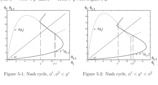
Example 1 Let < = 2, ; = 0-082, = = 1-5, ) = 0-6, (2& = 4023, / = 0-01, > = 0. Then
.* = 8-96, ""
= 10-87, and there is a two-cycle with .1 = 7-50' ""
and .2 = 10-56 ' ""
. See Figure 5-1.
Example 2 Same as Example 1 except== 1-1. Now.* = 9-35, ""
= 11-04, and there is a two-cycle .1 = 7-79' "" and.2 = 11-635 "" - See Figure 5-2. 0 2 4 6 8 10 12 0 2 4 6 8 10 12 ! 45o ! f -1(" t-1) ! f("t) " t-1 " t " t,"t-1 "2 "1 y*
Figure 5-1: Nash cycle, .1$ .2 ' ""
0 2 4 6 8 10 12 14 0 2 4 6 8 10 12 14 ! 45o ! f(" t) ! f -1(" t-1) " t-1 " t,"t-1 "1 y*"2 "t
Figure 5-2: Nash cycle, .1 ' ""
' .2
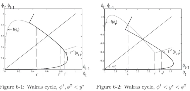
Example 3 Let <= 0-01, ;= 0-2, = = 1-5$ > = 2-5, ) = 0-4, (2&= 5029. Now.* = 0-61,
""
= 0-85, and there is a two-cycle with .1 = 0-44' ""
and.2 = 0-78' ""
. See Figure 6-1.
Example 4 Same as Example 3 except > = 5. Then .* = 0-70and""
= 0-92, and there is
a two-cycle with.1 = 0-43' ""
and.2 = 1-045 ""
0 0.2 0.4 0.6 0.8 1 0 0.2 0.4 0.6 0.8 1 y* "2 "1 ! f -1("t-1) ! f(" t) " t-1 " t " t,"t-1
Figure 6-1: Walras cycle, .1$ .2 ' ""
0 0.2 0.4 0.6 0.8 1 1.2 0 0.2 0.4 0.6 0.8 1 1.2 ! 45o ! f("t) ! f -1(" t-1) " t-1 " t " t, "t-1 "1 y* "2
Figure 6-2: Walras cycle,.1 ' ""
' .2
5.2
Chaos
Before discussing the economics behind results, we point out that our dynamical system can also generate higher-order cycles. Example 5 below shows a three-period cycle. The existence of a three-cycle implies the existence of cycles of all orders (Sarkovskii theorem) and chaotic dynamics (Li-Yorke theorem). Chaos is observationally equivalent to a stochastic process. Thus, credit limits and allocations can appear random, even though they are obviously deterministic in this perfect foresight economy. Proposition 6 below says that in any cycle
at least some periodic points are below""
, so the credit limit must bind at some point over
the cycle, although not necessarily all the time. Example 5 is a case in which. ' ""
in two
periods followed by one period in which. 5 ""
.
Example 5 Let <= 2-25, ;= 0-082,= = 1-3,) = 0-81, (2&= 4023, / = 0-01, > = 0. Now
.* = 16-65, ""
= 17-14, and there is a three-cycle with .1 = 15-73 ' ""
, .2 = 17-09 ' ""
and.3 = 18-935 ""
. See Figures 7 and 8.
Proposition 6 Suppose there is a unique stationary equilibrium with .* 5 0. In any ?
-period cycle, at least one -periodic point is binding, ."' "
"
14 15 16 17 18 19 20 14 15 16 17 18 19 20 y* " t-1 " t ! f -1(" t-1) ! 45o
Figure 7: A three-period cycle
0 10 20 30 40 50 60 70 80 90 100 15.5 16 16.5 17 17.5 18 18.5 19 19.5 t y* " t
Figure 8: Chaotic dynamics
5.3
Sunspots
The model can also generate stochastic cycles, in which credit limits and allocationsßuctuate
randomly over time, even though fundamentals (preferences, technologies and government policies) are deterministic and time invariant. If this is not animal spirits, we don’t know
what is. To illustrate we introduce a Markov sunspot variable @" " {1$2} for each ,. The
sunspot does not a"ect fundamentals, but as we show, it can still a"ect equilibrium. Let
Pr (@"+1 = 1|@"= 1) = A1 andPr (@"+1 = 2|@" = 2) =A2-The economy is in state @ if @"=@.
Let*!
* be type+’s value function in state@, and let(!*$ "*) be the allocation.
Agents now trade state-contingent credit contracts (!*$"$ "*$"), and we can write
**$"1 = %1(!*$"$ "*$") +) £ A***$"1+1+ (1#A*)*!1*$"+1 ¤ (24) **$"2 = %2("*$"$ !*$") +) £ A***$"2+1+ (1#A*)*!2*$"+1 ¤ - (25)
Contracts must satisfy the generalized participation conditions
%1(!*$"$ "*$")!0and %2("*$"$ !*$")!0$ (26)
plus the repayment constraint
&"*$" $.*$" %)(
£
A***$"1+1+ (1#A*)*!1*$"+1
¤
The relevant recursive representation is now .*$"!1 =A* % )( & % 1(! *$"$ "*$") +).*$" ¸ + (1#A*) % )( & % 1(! !*$"$ "!*$") +).!*$" ¸ - (28)
Under Nash bargaining, in state@at,we maximize%1(!*$"$ "*$")&%2("*$"$ !*$")1
!&
, subject
to the state-contingent repayment constraint. Equilibrium in state@ at date, is then given
by: if .*$" ' "'" then !*$" =0' ¡ .*$"¢ and"*$" =.*$" if .*$" !"' " then !*$" =0' ¡ "'"¢ and"*$" ="'" (29)
Under Walrasian pricing, agents maximize%1(!
*$"$ "*$")and%2("*$"$ !*$"), subject to budget
and repayment constraints. Equilibrium in state@ at date, is:
if .*$" ' "( " then !*$" =0( ¡ .*$" ¢ and"*$" =.*$" if .*$" !"( " then !*$" =0( ¡ "("¢ and"*$" ="(" (30)
DeÞnition 2 A sunspot equilibrium is given by nonnegative and bounded sequences of
credit limits©.*$"
ª#
"=1$*=0$1 and contracts{!*$"$ "*$"} #
"=1$*=0$1contingent on the state such that,
for for all , and@:
(i) (!*$"$ "*$") solves (29) or (30) given.*";
(ii) .*$" solves (28).
Using either of the pricing mechanisms, rewrite (28) as
.*$"!1 =A*6 ¡ .*$" ¢ + (1#A*)6 ¡ .!*$" ¢ $ (31)
where6 is deÞned as in the benchmark case. The economy is in aproper sunspot equilibrium
if .*$" 6=.!*$" for some ,. Consider equilibria that depend only on state, not the date, and
assume .2 5 .1. Then the repayment constraint is binding in state 1 (otherwise, we have
!* =!"
and"* =""
for both states, which implies.1 =.2). Following one standard methods
(see e.g. Azariadis 1981), the next result shows that proper sunspot equilibria exist for some parameters.
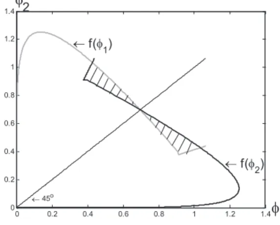
Proposition 7 Suppose there is a unique stationary equilibrium with .* 50. If 60(.*)'
#1 then there exist (A1$ A2), A1 +A2 ' 1, such that the economy has a proper sunspot
equilibrium in the neighborhood of .*.
0 2 4 6 8 10 12 14 16 0 2 4 6 8 10 12 14 16 ! 45o ! f("1) ! f("2) 0 2 4 6 8 10 12 14 16 0 2 4 6 8 10 12 14 16 ! 45o ! f("1) ! f(" 2) " 1 " 2
Figure 9-1 Nash sunspot equilibria
0 0.2 0.4 0.6 0.8 1 1.2 1.4 0 0.2 0.4 0.6 0.8 1 1.2 1.4 " 1 " 2 ! f(" 2) ! f(" 1) ! 45o
Figure 9-2: Walras sunspot equilibria
The condition 60(.*
) ' #1 in Proposition 7 is the same as the condition used for
two-period deterministic cycles. Hence, our previous examples of two-cycles also have sunspot
cycles. In Figure 9-1 and 9-2, the shaded area surrounded by 6(.1) and 6(.2) depicts the
set of (.1$ .2) that can be supported as sunspot equilibria for some A1 and A2, as stated in
the proposition.
6
Economics
The existence of equilibria with deterministic or stochastic cycles relies on the
nonmonotonic-ity of 6(."). To understand this, recall the dynamical system (21), which for convenience
we reproduce as
."=6¡."+1¢= )(
& %
1(!
"+1$ ""+1) +)."+1- (32)
An increase in credit limit at,+ 1 inßuences the economy at, in two ways. First it directly
when credit is easier tomorrow, agents will have more to gain from access to credit, so they will be less inclined to renege today and hence we can allow them more credit today. But
there is a second e"ect, since."+1 also a"ects%1(!"+1$ ""+1) on the RHS of(32). This e"ect
is ambiguous, in general, but as we mentioned earlier, it is negative when ."+1 is near "
"
under the mild assumptions of normal goods. In this case, easier credit tomorrow make
borrowers worse o", which makes them less inclined to honor their obligations today and
hence we can allow them less credit today. When this second, negative, e"ect is big enough
to dominate the Þrst e"ect, 6 is nonmonotone.
Proposition 8 If " is a normal good for type 1 and type 2 then in Nash equilibrium
1%1(!$ ")21. '0 for. =""#
4 for some4 50.
Proposition 9 If"is a normal good for type 2 then in Walrasian equilibrium1%1(!$ ")21. '
0 for. =""
#4 for some 4 50.
These results should not be too surprising. As remarked earlier, it is known that with nonlinear utility the Nash bargaining solution is not monotone: the surplus of an individual does not necessarily increase with the total surplus. As discussed in Aruoba et al. (2007),
this manifests itself in monetary theory with Nash bargaining by buyers being worse o"
when they have enough money to buy the analog of ""
than they would be if they had
just enough to buy ""
#4 (even when monetary policy is optimal, which means it is given
by the Friedman rule). Buyers are better o" when the constraint that they cannot spend
more money than they have binds slightly. Similarly, our borrowers are better o"when the
constraint that they cannot borrow more than their credit limit binds slightly. If we set
/ = 1, or if we use the proportional bargaining solution of Kalai instead of Nash, since these
imply agents’ surpluses are monotone in the total surplus we cannot get this e"ect. Hence,
Lest one is suspicious of results arising from nonmonotonicity or other curious properties of particular bargaining solutions, let us turn to Walrasian pricing. In this case, when the
credit limit is relaxed around "" #
4, the supply of " increases, which means relaxes type
1’s credit constraint. This makes him better o" at Þxed prices, but for small 4 this has
only a second-order e"ect on utility (the envelope theorem). The dominant e"ect is that
the terms of trade turn against him: when he is able to promise a bigger ", he may get
more !, but even if he does it is not enough to compensate for the bigger repayment. To
put it another way, in Walrasian equilibrium a buyer of good " is always better o" under
the restriction " $ "" #
4 for some 4 5 0, for the same reason that monopolists produce
less than perfectly competitive suppliers. In our Walrasian equilibrium agents are perfectly competitive, so they cannot unilaterally impose quantity restrictions to move prices in their favor, but endogenous credit limits based on limited commitment can get the the job done
for them.13
While credit constraints can make borrowers better o", they cannot make everyone better
o". Propositions 2 and 3 imply(!$ ")"C¯with Walrasian pricing, and with Nash bargaining
at least if / is not too high. When . is reduced around "" #
4, someone has to lose, which
has to be type 2, the lenders in our economy. Of course, when credit limits are too tight
they make everyone worse o"(consider. = 0), but they make borrowers better o"if not too
tight. As we said above, when credit limits are not too tight, loosening them tomorrow makes
borrows worse o"tomorrow, and hence more inclined to renege today, which imposes stricter
credit constraints today. Notice in (32) that this negative e"ect of ."+1 on ." is ampliÞed
by (2&, so if (2& is large then 6(.) is decreasing around ""
. By choosing )(2(1#))&
appropriately — i.e., close to ""
2%1(!"
$ ""
) — we can ensure that stationary equilibrium is
near ""
, which makes it easy to guarantee the critical condition60(.*)'#1for endogenous
13By analogy, in a competitive labor market no individual worker can cause a wage increase by restricting
his own labor, but a union can do so by restricting everyone’s labor. Our endogenous credit limit similarly gives our borrowers some market power.
dynamics. And because we have some freedom in choosing(,&, our results do not dependent
critically on)or the curvature of the utility function as they do in other models; risk aversion
and discounting in our examples are quite reasonable.
In cyclic equilibria, welfare as measured by*! for type+ varies over the cycle. It turns out
that sometimes cycles Pareto dominate stationary equilibria; sometimes stationary equilibria dominate cycles; and sometimes they are noncomparable.
Example 6 (continuation of example 4). In stationary equilibrium, *1 = 0-28 and *2 =
0-73. In the two-cycle starting at.1 = 0-43,*1 = 0-47and*2 = 0-79, which dominates the
stationary equilibrium. But starting with.2 = 1-04,*1 = 0-19and*2 = 1-08, which is not
comparable with the stationary equilibrium.
Example 7 (continuation of example 5). In stationary equilibrium, *1 = 1-54 and *2 =
83-51. In the two-cycle starting at .1 = 16-17, *1 = 1-65 and *2 = 83-08, which is not
comparable with the stationary equilibrium. But starting with .2 = 17-79, *1 = 1-50 and
*2 = 83-39, which is dominated by the stationary equilibrium.
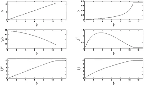
Figures 10 and 11 show how in Examples 1 and 3. a"ects!,",%1,%2 and% =%1+%2
(note that summing utilities makes sense, as the examples are quasi-linear). They also
show how . a"ects the terms of trade, or the interest rate B = "2!.14 These are “partial
equilibrium” experiments, showing how certain endogenous variables depend on another
endogenous variable., but dynamic equilibria can be interpreted as moving along the curves.
In the examples, both!and"increase until. hits""
. The payo"of the lender%2 increases
with ., while the payo" of the borrower %1 Þrst increases then decreases.15 Note that %1
14In Walrasian equilibrium, in general, the budget equation is .
$#+! = .$#¯+ ¯! where #¯ and !¯are
endowments and we normalize.%= 1(note that#and.$could be vectors here). Represent this recursively
as #= ¯##1 and ! = ¯!+12, where 1 is saving and 2 is the gross interest rate. Eliminating 1 implies
#= ¯##(!#!¯)-2. Hence,2=.$, and in our economy.$=!-#by type2’s budget equation.
15One can show"2 increasing in(for(near!", and"! increasing for(near0. Indeed, with Walrasian
not only decreases near ""
, as guaranteed by Propositions 8 and 9, it decreases over a wide
range of .. A di"erence between the Figures is the behavior ofB. With Walrasian pricing,
Figure 9 showsB increasing with., which as we discussed is the reason%1 decreases. With
Nash bargaining, Figure 8 shows B decreasing in ., and in this case %1 falls with . for a
di"erent reason, the nonmonotonicity of the Nash solution.
Figure 10: Example 1 continued
Finally, Figure 12 shows time series for the endogenous variables in the example with
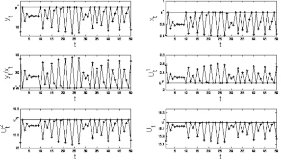
chaotic dynamics. These series are consistent with the idea that the economy ßuctuates
between normal times, when credit is easy in the sense that. is high andB low, and crunch
time, when the opposite is true. This is driven exclusively by beliefs. While some agents
(borrowers in this example) are better o" in a credit crunch, others (lenders) are worse o",
and since quasi-linear utility allows us to measure total welfare, we can meaningfully say
that the economy as a whole is worse o"in a crunch. This example may be too “regular” to
match actual data — but it is, after all, only an example. Still, a message one might take away from this is that it can be hard to explain actual data purely with animal spirits, at least
in a model as simple as this. This suggests that it may be useful to combine self-fulÞlling
beliefs with changes in fundamentals. Once it is understood that beliefs can generate credit cycles, with no change in preferences, technologies or policies, it must be acknowledged that they can also amplify or propagate shocks to fundamentals.
7
Conclusion
We developed a framework to study credit market dynamics. There is no fundamental uncertainty, although in principle this would be easy to add. Still there exist multiple equilibria, including deterministic, chaotic, and stochastic credit cycles. This illustrates how agents’ beliefs — animal spirits or extrinsic uncertainty — can play an important role in credit markets. Our model contains ingredients that we think are particularly relevant for recent events, including imperfect collateral and imperfect monitoring. Even with these features in the framework, it is still quite tractable. Moreover, in the examples presented, the existence of endogenous credit market dynamics does not depend on unrealistic parameter values. Perhaps endogenous credit cycles are more pervasive than we used to think.
Appendix A
Proof of Proposition 1: DeÞne C (.) = 6(.)#.- Our parametric assumption implies
C0(0) 5 0. Also, C0(.) ' 0 for . 5 ""
. By the continuity and monotonicity of C (.) for
. 5 ""
, it is easy to see the following: if C (""
) ! 0 then there exists .* 5 ""
such that
C (.*) = 0; and ifC(""
)'0then there exists at least one.* in(0$ ""
) such thatC (.*) = 0.
In the latter case, there is no stationary equilibria in which.*5 ""
, becauseC(.)is strictly
decreasing for . 5 ""
. ¥
Proof of Proposition 2: When / = 1, bargaining equilibrium is the same as the planner’s
allocation with%2(!$ ") = 0. When / = 0, (!$ ") = (0$0)is the equilibrium.
Case 1: The repayment constraint is not binding at / = 1. The unconstrained
equi-librium (!$ ") " C¯is continuous in / and has the property that 1!
1/ 5 0 and 1"
1/ ' 0. The
repayment constraint becomes binding at some ˆ/ " (0$1). Denote the equilibrium at ˆ/ by
(ˆ!$"ˆ)-For/ 'ˆ/, the repayment constraint is binding. Equilibrium is characterized by
/%#1(!$ 7(!))%2(7(!)$ !) + (1#/)%1(!$ 7(!))%#2(7(!)$ !) = 0- (33)
If / = 0 then ! = 0, and if / = ˆ/ then ! = ˆ!. Because ! is continuous in /, for any
! " [0$!ˆ] there exists / " h0$ˆ/i s.t. (33) is satisÞed. Because the allocation is below the
core )#1(#$%) !)1 "(#$%) 5 !)2 #(%$#) )2 "(%$#) .
Case 2: The repayment constraint in binding at / = 1. By repeating the argument in
case 1 for / 'ˆ/, we conclude the set of equilibrium allocations for / " [0$1] is that part of
the repayment constraint below the core. ¥
Proof of Proposition 3: Let (!*$ "*) be a stationary equilibrium allocation. There two
cases.
Case 1: "* ' 7(!*). The equilibrium is on the contract curve and in the constrained
core.
2’s indi"erence curve and the repayment constraint) in Figures 2-1 and 2-2. Denote the
allocation at:by(˜!$"˜). The equilibrium(!*$ "*)solves!=0( (")and"=7(!)-The slope
of type 2 agent’s indi"erence curve at the equilibrium(!*$ "*) is
#%2 #("*$ !*) %2 % ("*$ !*) = " * !* = 7(!*) !* = +, - % 1(!*$ "*) !* - (34)
The Þrst equality is simply ! = 0( ("); the second follows from "* = 7(!*); the last from
the deÞnition of7(!)- The slope of7(!*) is
70(!*) = +, - % 1 #(!*$ "*) 1#+,- %1 % (!*$ "*) - (35)
Because %1(!$ ") is concave in !, we have
+, - % 1(!*$ "*) !* 5 )( & % 1 #(!*$ "*)- (36)
By the fact that%1
% '0, we have )( & % 1 #(! *$ "*)5 +, - % 1 #(!*$ "*) 1# +, - %%1(!*$ "*) - (37) Combining (34)#(37), #% 2 #("*$ !*) %2 % ("*$ !*)
5 70(!0)- Therefore, type 2’s indi"erence curve at !*
intersects 7(!) from below. The planner’s allocation(˜!$"˜) satisÞes70(˜!) = #%
2
#(˜"$!˜)
%2
% (˜"$!˜)
. By
the concavity of7(!) and convexity of type 2’s indi"erence curve,!* 5!˜.
¥
Proof of Proposition 4: Because 6(.") is continuous, ."!1 covers the interval
h
0$˜.i for
." "[0$ . *
]. Since there is a unique positive stationary equilibrium6(.")5 ."for." "(0$ .
*
) and 6(.") ' ." for ." " (.*$)). That is .
"!1 5 ." for ." " (0$ .
*) and .
"!1 ' ." for
." "(.*$)). Given .
0 '.˜, there is a.1 such that .1 "(0$ .*) and.1 ' .0, which implies
a .2 "(0$ .*) with .2 ' .1, and so on. This decreasing sequence{."}
#
0 converges to0. ¥
Proof of Proposition 5: Let62(.) =6*6(.). Because.*
is the unique positive stationary
for . 5 ""
, there exists a . 5 "˜ "
such that 6³˜.´ 5 ""
. By the uniqueness of the positive
stationary equilibrium, 62³.˜´' 6³.˜´'˜.. The slope of62(.*
)is 962(.* ) 9.* =6 0[6(.* )]60(.* ) =60(.* )60(.* ) = [60(.* )]2 51
-The last inequality follows from60(.*
)'#1. Similarly,62(0) = [60(0)]2 50-By continuity,
62 must cross the 45 degree line in(0$ .*
). Because62 lies below the diagonal at.˜, it crosses
it at least once in ³.*$.˜´. Therefore, there are two more Þxed points (in addition to 0 and
.*) such that0' .1 ' .* ' .2 for 62(.). ¥
Proof of Proposition 6: Let .1$ .2$..., .1 be the periodic points of a ?-period. We prove
the proposition in two steps.
Step 1: At least one periodic point is less than .*.
Prove by contradiction. Suppose instead all periodic points are larger than .*. By the
deÞnition of a ?#period cycle,
.1 =6(.1)' .1
The inequality follows from the fact that 6(.) ' . for . 5 .* by the uniqueness of the
positive stationary equilibrium. Repeat the procedure starting from.1 to get
.1=6¡.1!1¢' .1!1 =6¡.1!2¢' .1!2---- ' .1
-A contradiction.
Step 2: There does not exist a cycle if .* 5 ""
.
Prove by contradiction. Suppose instead there is a cycle and .* 5 ""
. By step 1, there
exist at least one periodic point larger than .*. Let .1 5 .*- The periodic point .2 5 .*
because
.2 =6¡.1¢5 6(.*) =.*
The inequality follows from the fact the 6 is strictly increasing for . 5 ""
. Repeat the
We conclude from steps 1 and 2 that if there exists a cycle, . must be binding in some,
if not all, periods. ¥
Proof of Proposition 7: Because 6 is decreasing around .*, there exists an interval
[.*#41$ .*+42]$ 41$ 42 50, such that6(.1)5 6(.2)for.1 "[.
*#
41$ .*),.2 "(.
*
$ .*+42].
By deÞnition(.1$ .2),.1 6=.2, is a proper sunspot equilibrium if there exist(A1$ A2),A1$ A2 '
1, such that
.1 = A16(.1) + (1#A1)6(.2) (38)
.2 = (1#A2)6(.1) +A26(.2)- (39)
Because.1 and.2 are weighted average of6(.1)and6(.2), and6(.1)5 .1and6(.2)' .2
by the uniqueness of the positive stationary equilibrium, necessary and su!cient conditions
for (38)and(39) are
6(.2) ' .1 ' 6(.1)$ (40)
6(.2) ' .2 ' 6(.1)- (41)
Because .1 ' .2 we can reduce(40) and(41) to
.2 ' 6¡.1¢$ (42)
.1 5 6¡.2¢- (43)
Expanding 6(.1)and6(.2)around .* and using 6(.*) =.*,(42)#(43)are equivalent
to .2#.* .*#. 1 '#60(.* )' . *# .1 .2#.*$ Because #60(.* )51, 32!3 $ 3$!3 1 '#6 0(.* ) is redundant if #60(.* )' 3$!31
32!3$. Now we have two
unknowns (.1$ .2) and only one inequality #60(.*) ' 3$!3
1
32!3$ to solve. It is straightforward
that multiple solutions exist on[.*#4
as A1 +A2 = .1#6(.2)#.2+6(.1) 6(.1)#6(.2) = .1#.2 6(.1)#6(.2)+ 1 '1$ because 31!32 4(31)!4(32) is negative. ¥ Proof of Proposition 8: If . = ""
, the equilibrium is on the contract curve and %
1 # #%1 % = #%2 # %2 % . Thus, (13) evaluated as .("" ! is 1%1(!$ ") 1. ¯ ¯ ¯ ¯3$%! " + /%2%1 % ³ %1 ### )1 # )1 "% 1 #% ´ + (1#/)%1%1 % ³ %2 ### )2 # )2 "% 2 #% ´ /(%1 ##%2+%#1%#2) + (1#/) (%#1%#2+%1%##2 )
The denominator is negative. The numerator is positive if " is normal for type 1 and type
2. ¥
Proof of Proposition 9: If . = ""
, equilibrium is on the contract curve and %
1 # #%1 % = #%2 # %2 % = " !. Thus, (20) evaluated as .(" " ! is 1%1(!$ ") 1. ¯ ¯ ¯ ¯3$%! " = % 1 % ! & '! 2%2 ##+ 2!"%#%2 +"2%%%2 %2 # +! ³ %2 ### )2 # )2 "% 2 #% ´ ( )
-The term outside the brackets is negative. -The term in brackets is positive as long as " is
Appendix B
Consider a stationary allocation (!$ ") " C. We show it can be dominated by a time-¯
varying allocation if the stationary repayment constraint is binding, " = 7(!), but type
2’s participation constraint is not, %2("$ !) 5 0. For this we use quasi-linear preferences,
%1(!$ ") =E(!)#" and%2("$ !) ="#F(!).
Since " = 7(!) binds, ! ' !"
. Consider an alternative allocation (!1$ "1) = (!$ "+41),
(!2$ "2) = (!+G$ "#42), and (!"$ "") = (!$ ") for , ! 3. We claim there exists (41$ 42$ G)
such that this dominates the original allocation. The di"erence in payo"s in the two original
allocations for type 1 is !*1 =)[E(!+G)#E(!)]#4
1 +)42, and for type 2!*2 =41#
)42+)[F(!)#F(!+G)]. Set!*2 = 0, so!*1 =)[E(!+G)#F(!+G)]#)[E(!)#F(!)].
Because ! ' !"
, we can Þnd G such that !*1 50.
Next, we show (!1$ "1) and(!2$ "2) are feasible for some (41$ 42$ G). By construction, the
repayment constraint at,= 2, all participation constraints for type1, and the participation
constraints for type2at,= 1hold. It remains to check 2’s participation constraint at, = 2,
*22 ="#42#F(!+G) +
)
1#)%
2("$ !)!0$ (44)
and the repayment constraints at ,= 1,
)( &% 1(! 2$ "2) + )2 1#) ( &% 1(!$ ")!" 1- (45) Rewrite (44) to get 1 1#)% 2("$ !) +F(!)#F(!+G)#4 2 !0 (46) Because %2("$ !) 5 0, we can Þnd 4
2 and G to satisfy (46). Using 1!++
, -% 1(!$ ") = " to rewrite(45), we get )( &[E(!+G)#E(!) +42]!41 (47)
References
[1] Akerlof, G. and R. Shiller (2009), Animal Spirits: How Human Psychology Drives the
Economy, and Why it Matters for Global Capitalism, Princeton University Press.
[2] Aliprantis, C., Camera, G. and Puzzello, D. 2006. “Matching and Anonymity,”
Eco-nomic Theory 29, 415-432.
[3] Aliprantis, C., Camera, G. and Puzzello, D. 2007. “Anonymous Markets and Monetary
Trading,” Journal of Monetary Economics 54, 1905-1928.
[4] Alvarez, F. and U. Jermann (2000), “E!ciency, Equilibrium, and Asset Pricing with
Risk of Default,”Econometrica 68, 775-797.
[5] Aruoba, B., G. Rocheteau and C. Waller (2007) “Bargaining and the Value of Money,” Journal of Economic Theory 54, 2636-2655.
[6] Azariadis, C. (1981) “Self-fulÞlling Prophecies,” Journal of Economic Theory 25,
380-396.
[7] Azariadis, C. (1993) Intertemporal Macroeconomics, Blackwell.
[8] Azariadis, C. and L. Kaas (2007) “Asset Price Fluctuations without Aggregate Shocks,” Journal of Economic Theory 136, 126-143.
[9] Azariadis, C. and L. Kaas (2008) “Endogenous Credit Limits with Small Default Costs,” Mimeo, Washington University.
[10] Ferguson, N. (2008), The Ascent of Money, Penguin Press.
[11] Bertaut, C. and M. Haliassos (2002) “Debt Revolvers for Self Control,”Mimeo,
[12] Gertler, M. and N. Kiyotaki (2010) “Financial Intermediation and Credit Policy in
Business Cycle Analysis,” forthcoming in Handbook of Monetary Economics, Second
Edition.
[13] Haliassos, M. and M. Reiter (2005) “Credit Card Debt Puzzles,” Mimeo, University of
Cyprus.
[14] Hellwig, C. and G. Lorenzoni (2009) “Bubbles and Self-Enforcing Debt,”Econometrica
77, 1137—1164.
[15] Kalai, E. (1977) “Proportional Solutions to Bargaining Situations: Interpersonal Utility
Comparisons,”Econometrica 45, 1623-1630.
[16] Kehoe, L. and D. Levine (1993) “Debt-constrained Asset Markets,”Review of Economic
Studies 60, 865-888.
[17] Kehoe, L. and D. Levine (2001) “Liquidity Constrained Markets versus Debt
Con-strained Markets,” Econometrica 69, 575-598.
[18] Kiyotaki, N. and J. Moore (1997) “Credit cycles,” Journal of Political Economy 105,
211-248.
[19] Largos, R. and R. Wright (2005) “A UniÞed Framework for Monetary Theory and Policy
Analysis,” Journal of Political Economy 113, 463-484.
[20] Laibson, D., A. Repetto and J. Tobacman (2001) “A Debt Puzzle,” Mimeo, Harvard
University.
[21] Lorenzoni, G. (2008) “Ine!cient Credit Booms,”Review of Economic Studies 75, 809—
[22] Lucas, R. and E. Prescott (1974) “Equilibrium Search and Unemployment,” Journal of Economic Theory 7, 188-209.
[23] Mattesini, F., C. Monnet and R. Wright (2010) “Banking: A Mechanism Design
Ap-proach,” Mimeo, Federal Reserve Bank of Philadelphia.
[24] Mortensen, D. and C. Pissarides (1994) “Job Creation and Job Destruction in the
Theory of Unemployment,” Review of Economic Studies 61, 397-415.
[25] Nosal, E. and G. Rocheteau (2010) Money, Payments and Liquidity, MIT Press,
forth-coming.
[26] Rocheteau, G. and R. Wright (2005) “Money in Search Equilibrium, in Competitive
Equilibrium, and in Competitive Search Equilibrium,” Econometrica 73, 175-202.
[27] Sanches, D. and S. Williamson (2010) “Money and Credit with Limited Commitment
and Theft,” Journal of Economic Theory 145, 1525-1549.
[28] Williamson, S. and R. Wright (2010a) “New Monetarist Economics: Methods,” Federal
Reserve Bank of St. Louis Review 92(4), 265-302.
[29] Williamson, S. and R. Wright (2010b) “New Monetarist Economics: Models,”