On Interference-aware Provisioning for Cloud-based
Big Data Processing
Yi YUAN
∗, Haiyang WANG
†, Dan Wang
∗, Jiangchuan LIU
† ∗The Hong Kong Polytechnic University,†Simon Fraser UniversityAbstract—Recent advances in cloud-based big data analysis
offers a convenient mean for providing an elastic and cost-efficient exploration of voluminous data sets. Following such a trend, industry leaders as Amazon, Google and IBM deploy various of big data systems on their cloud platforms, aiming to occupy the huge market around the globe. While these cloud systems greatly facilitate the implementation of big data analysis, their real-world applicability remains largely unclear.
In this paper, we take the first steps towards a better understanding of the big data system on the cloud platforms. Using the typical MapReduce framework as a case study, we find that its pipeline-based design intergrades the computational-intensive operations (such as mapping/reducing) together with the I/O-intensive operations (such as shuffling). Such computational-intensive and I/O-computational-intensive operations will seriously affect the performance of each other and largely reduces the system effi-ciency especially on the low-end virtual machines (VMs). To make the matter worse, our measurement also indicates that more than
90% of the task-lifetime is in the shadow of such interference. This unavoidably reduces the applicability of cloud-based big data processing and makes the overall performance hard to predict. To address this problem, we re-model the resource provisioning problem in the cloud-based big data systems and present an interference-aware solution that smartly allocates the MapReduce jobs to different VMs. Our evaluation result shows that our new model can accurately predict the job completion time across different configurations and significantly improve the user experience for this new generation of data processing service.
I. INTRODUCTION
Nowadays, big data systems have already formed the core of technologies powering enterprises like IBM, Yahoo! and Facebook. To address the costly system deployment and man-agement problem faced by small enterprises, who also want to enjoy big data technique, cloud-based big data analysis has been widely suggested. It enables elastic services framework to the users in a pay-as-you-go manner, and largely reduces their deployment and management costs.
The cloud systems were initially designed to provide re-mote and virtualized services (accomplished by virtual ma-chines (VMs)), where the resources and capacities are speci-fied by the users). To accommodate the increasing number of applications and workloads to be settled on cloud, the design of cloud is intrinsically distributed to promote parallelism, i.e., scaling out (add more servers) rather than scaling up (upgrade the servers). In addition, providing stable virtualized services is critically important for cloud providers, i.e., having the same payment and the same amount of resources/capacities, the users expect similar services (e.g., finishing time for their jobs). While the cloud is providing satisfactory services for current applications such as web services etc, it remains
largely unclear whether a straightforward application of big data systems on cloud will be satisfactory.
In this paper, we take the first steps towards a comprehensive understanding of the big data systems on the cloud platform. Using the typical MapReduce framework[1] as a case study, our real-world experiment shows that a few high-end VMs can, achieve better performance comparing to a number of low-end VMs with identical lease cost (also with the same total capacity). In particular, while processing a35.7Gigabytes data on Amazon EC2, 2 extra large instances can complete the MapReduce job more than 10% faster than that of 16 small ones. To better understand such an observation, we take a closer look into the cloud-based MapReduce systems. We find that the pipeline-based design of MapReduce inter-grades the computational-intensive operations (such as map-ping/reducing) together with the I/O-intensive operations (such as shuffling). Unfortunately, such computational-intensive and I/O-intensive operations will seriously affect the performance of each other and largely reduces the system efficiency espe-cially on the smaller VMs. In the case of MapReduce, when the EC2 VMs are generating and shuffling the intermediates, such computational-intensive operations as mapping and re-ducing will also be invoked; the great amount of input data will only enlarge their mutual-interference, potentially leading to longer job completion time. This will introduce serious problems to the cloud-based big data systems such as service maintenance. To make the matter worse, our measurement also indicates that more than 90% of the job-lifetime is in the shadow of such interference. This unavoidably reduces the applicability of cloud-based big data processing and makes the overall performance hard to predict.
The cloud rarely faces such problem previously as there is seldom task that is both computational-intensive and I/O-intensive (we observe that for a typical big data task with an input of 35.7GB, the intermediate data generated can be as much as 70GB+). 1 As such, existing solutions fails to
provide satisfactory resource provisioning for cloud-based big data applications. To address this problem, we re-model the resource provisioning problem and present an interference-aware solution that smartly allocates the MapReduce jobs to different VMs. Our evaluation results show that our solution can effectively reduce the job completion time for the new big data processing service.
1This interference also does not exist (or to a much lower degree) if MapReduce runs on conventional physical machines. This is because if run-ning on physical machines, MapReduce tasks are stand-alone and intrinsically distributed; a sharp contrast to the virtualized cloud environment.
2000 2500 3000 3500 0 0.2 0.4 0.6 0.8 1
Job Completion Time (second)
CDF
Small−16 XLarge−2
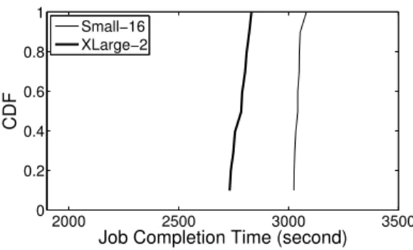
Fig. 1: The cumulative distribution of processing time for same MapReduce job under different cluster configuration on our clusters built with EC2 instances. All configurations have same computing capacity.
II. CLOUDDEPLOYMENT OFMAPREDUCE
We will first discuss MapReduce in details and how it can be applied to the cloud environment. We then show that VM selection can become a challenging task.
A. MapReduce and Cloud Deployment
The process of a MapReduce job consists of three phases:
map, shuffle and reduce. There are two program functions:
mapper andreducer. In the map phase, the input data is split into blocks; the mappers then scan the data blocks and pro-duce intermediate data. In the shuffle phase, the MapRepro-duce framework shuffles intermediate data and move them to the correct node for reducing. After that, the reducers process the shuffled intermediate data and generate results in reduce phase. We call the operations in each phase asmapping,shufflingand
reducing. In a given MapReduce system, these operations are invoked in different tasks/processes. For example, in Hadoop, there are two types of tasks:map taskandreduce taskwhere the mapping is done by map tasks, shuffling and reducing are done by reduce tasks2.
To deploy a real-world MapReduce system, a dedicated server cluster is required. A typical MapReduce cluster con-sists of two types of machines:masterandslave. There is only one master in the cluster; this master assigns map and reduce tasks to the slaves after the MapReduce jobs are received. Afte that, it will further monitors the tasks on the slaves (for example, handling possible task failures). There are multiple slaves in the cluster. These slaves are deployed to run map and reduce tasks assigned by the master.
B. Challenges in VM Selection
While the cloud can eliminate the load of maintenance of physical machines, the users still need to make VM selections for their respective big data processing tasks. Such VM selection and renting are critical as they directly influence the budget constraint and job completion time. Current resource provisioning in cloud is based on workloads, where the virtu-alized CPU capacity acts as the main factor. Such provisioning works well for such applications as web services, etc.
2There are some supporting tasks which cooperate with map and reduce tasks. For example, TaskTrackers monitor and schedule map and reduce tasks.
We conduct a more comprehensive experiment and show that there are considerable interferences in big data applica-tions on cloud platform. This indicates that VM selection may not be a straightforward task. Our experiments are as follows. We apply EC2 to build our experimental MapReduce clusters. We employ Wordcount as the MapReduce program in our experiments. Wordcount aims to count the frequency of words appearing in a data set. It is one of the most classic MapReduce jobs which serves as the basic component of many Internet applications (e.g. document clustering [2], searching, etc). In addition, most MapReduce jobs have aggregation statistics closer to Wordcount [3]. To provide a fare comparison to the existing studies [4][5], we apply the document package from Wikipedia as the input data. This package contains all English documents in Wikipedia since30th January 2010 and the size
of uncompressed data is 35.7 GB. Moreover, we use the the most popular version of Hadoop1.0.3to build the MapReduce cluster in our experiments.
We use two types of EC2 VMs in our experiments: Small instanceandExtra Large (XLarge) instance. The capacity as well as the lease cost of one XLarge instance is approximately equal to 8 Small instances. This can help us better compare the trade-off between performance and cost. Because input data are stored on a distributed file system, which is typically on slaves, and these data are processed by tasks on slaves, the performance of a MapReduce cluster is mainly decided by the slaves. Meanwhile, master works as coordinator of slaves and does not take CPU-intensive task, so when we choose configuration for a cluster, we choose instance types for master and slaves separately. We fix the type of master as Small. After that, we adjust the type as well as the total number of slaves. For the sake of clarity, we use the type as well as the total number of slaves to identify each experiment. For example,Small-16 indicants that there are16EC2 Small instance running as slaves in the experiment.
We deploy two MapReduce clusters Small-16 and XLarge-2 on the EC2 platform. As we can see in Fig.1, when we employ 2XLarge instances in our cluster, the job can be done between 2732 to 2831 seconds. On the other hand, when we use 16 Small instances, the job completion time will be increased to around3042 seconds. This experimental result indicates that the users will suffer from a 10%capital loss by using VMs with smaller capacities.
III. MEASUREMENT
To better understand the underlying reasons of job comple-tion time difference caused by VM seleccomple-tion, we answer two questions in this section: 1) what are the unique features of big data applications such as Mapreduce; and 2) how these features bring new challenges to the cloud deployments.
A. Analysis of MapReduce Processes
They are many existing studies dedicated on the investi-gation of MapReduce processes [6][7][8]. These studies are mostly focusing on the stand-alone measurements of the CPU,
0 50 100 T o t a l I / O R a t e ( M b p s ) 0 0 50 100 D i s k I / O R a t e ( M b p s ) 0 500 2500 3000 0 20 40 N e t w o r k I / O R a t e ( M b p s ) 0 0 50 100 150 C P U u s a g e ( p e r c e n t a g e ) (a) (b) (c) (d) MS MO RO 0
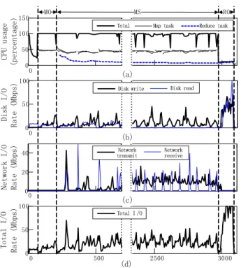
Fig. 2: MapReduce process. (a) CPU usage; (b) Disk I/O usage; (c) Network I/O usage; (d) Total I/O usage. Results from 700s to 2300s are omitted.
the memory, the disk I/O and the bandwidth utilization. How-ever, the relationships between these tasks remain unclear for the general public. To this end, our measurements emphasize on the interactions between mapping, shuffling and reducing operations. We synchronize the CPU, disk I/O as well as the network traffic based on a standardized time line to provide a closer look into the MapReduce system.
Fig.2(a)-(d) show the CPU utilization, disk I/O, network I/O and total I/O on one slave used in the previous discussed Small-16 experiment. In Fig.2(a), the fine lines and the dashed lines indicate the CPU utilization of map and reduce tasks respectively. The dark line shows the total CPU utilization. It is easy to see that there are three main stages in this figure: 1) Mapping only stage (MO stage) from 90 to 215 seconds. In this stage, only map tasks are running. 2) Mapping-Shuffling stage (MS stage) from the end of MO stage form 215 to 2963 seconds. In this stage, map tasks and reduce tasks are overlapped and running together. Note that the reduce task is shuffling intermediate data in this stage. 3) Reducing only stage (RO stage). The RO stage is from 2963 to around 3081 seconds. In this stage, map tasks are finished and only reduce tasks are running. Beside these three stages, there are preparing time and closing time at the head and tail of the process.
In Fig.2(a), we see that the CPU is fully utilized during MO and MS stages. The total CPU usage reaches 100%. This is because Hadoop enables multiple map tasks and one reduce task on this slave. When the first map task in MO stage is finished, reduce task will be started and runing in parallel with the remaining map tasks.
In Fig.2(b), we see that disk reading operations start from
the beginning of the job and last until the end. Meanwhile, disk writing operations are found shortly after map tasks start. These operations stays at a high rate to read input data, store/read intermediate data and store final results to disk. Compared with disk I/O, network operations (see Fig.2(c)) are more pulsed.
Note that the disks in cloud are network-attached. As a result, disk I/O and network I/O operations in virtualized instance are merged into network I/O-intensive operations at underlying cloud implementation. After we merge disk I/O and network I/O in Fig.2(d), we see that I/O operations starts from the very beginning and I/O rate increases in every stage. In particular, the I/O rate starts from 10 Mbps and then increases to about 18 Mbps in MO stage. After that, the I/O rate grows to around 30 Mbps in MS stage. Finally, it elevates to over 100 Mbps in RO stage. From Fig.2(a) and Fig.2(d), we see that a typical MapReduce job is both computational-intensive and I/O-intensive at slaves.
B. Interference Between CPU-intensive and I/O-intensive Tasks
Based on our measurements, we can see that the MapRe-duce processes are both CPU-intensive and network I/O-intensive. In this sub-section, we will further clarify whether such a feature will introduce new challenges to the cloud deployment.
To this end, we run a standard CPU benchmark [9] on a EC2 Small instance. We adjust the traffic load on this VM and check the running time of this benchmark. To provide a fare comparison, we also apply same experiment on a local physical machine (non-virtualized server). The local machine have identical (even weaker in terms of compute capacity) hardware configuration to the EC2 Small instance. Fig.3 shows the comparison between EC2 Small instance and our local server. From this figure, we can see that the traffic load slightly increases benchmark running time on the non-virtualized server, . e.g. When traffic load changes from 0Mbps to 250Mbps, the running time of CPU benchmark is increased by 20%. However, for the virtualized EC2 small instance, the benchmark running time is increased by 45% under the same traffic load. Furthermore, we also test the case in EC2 extra large instances(see Fig.4). Since the XLarge instance has 8 ECUs while small instance has 1 ECU, we run 8 parallel cpu benchmarks on XLarge instance. When traffic load is zero, benchmark running times on both Small instance and XLarge instance is7.2ms with very small standard derivation. This means the CPU resource allocation of EC2 is accurate when there is no traffic load. When traffic load grows, we can see that the small instance will suffer from remarkable performance degradation while the benchmark running of XLarge instance is only slightly increased.
This result can be interpreted from two aspects. From the network aspect, it is known that the network performance of virtualized instance is unstable in cloud environment [10]. The abnormal delay variations in network communication makes operating system spend more CPU processing time on
0 100 200 300 400 0 20 40 60 80 Traffic load (Mbps) Increase in CPU benchmark running time (percentage)
Virtualized EC2 server (small) Non−virtualized server
Fig. 3: Increasing of CPU bench-mark running time on Small in-stance and physical machine.
0 200 400 600 800 1000 7 8 9 10 11 12 13 Traffic load (Mbps) CPU benchmark
running time (second)
Small XLarge
Fig. 4: CPU benchmark running time on Small and XLarge in-stances.
handling such network traffic. Therefore, the CPU time allo-cated to other tasks will be reduced. Moreover, the virtualized network device queuing [11] is another important factor. From the CPU aspect, it is known that VMs are sharing physical processors on cloud platform [12]. The smaller a VM is, the easier it will suffer from resource competition with other VM (located in the identical physical server). This is the reason why large VMs have much lower probability to confront such an interference.
IV. RESOURCEPROVISIONING OFCLOUD-BASED
MAPREDUCE
Based on the experimental results, we can see that the task interferences do not exist in conventional physical machines (or to a much lower degree) in Fig.3. As such, the existing cloud-based big data studies mainly focus on the optimization of stand-alone workloads, without considering their interfer-ence in the virtualized environment.
A. Modeling of Interference-aware Resource Provisioning
In order to remodel resource provisioning problem with considering interference in cloud. We remodel completion time of a MapReduce job first. Our model is based on the existing MapReduce model in [13] where the job completion time is modeled in Eq.1. Note that this model is extensively evaluated on real world MapReduce clusters.
t=M(M O)+ (NM
SM
−1)M(M S)+NRR
SR
+C0 (1) The first partM(M O)is the running time of MO stage. The second part(NM
SM−1)M
(M S)
is the running time of MS stage.
NMis the number of map tasks determined by the size of input
dataDand data block sizedM.M is the average running time
of map tasks. SM is the total number of in-parallel map task
in the cluster where SM < NM. The third part, NSRRR, is the
running time of RO stage. NR is the number of reduce tasks
in the job. R is the average running time of reduce tasks in RO stage.SRis the total number of in-parallel reduce task in
the cluster whereSR< NR. The last partC0is a constant. It
represents the preparing time and the closing time.
To scale the model with input data size,Ris further modeled as R=C1+C2dR.dR is the average amount of intermediate
data processed per reduce task.C1 andC2 are scaling factors for the reduce tasks. dR can be adjusted according to total
amount of input data and NR. In particular, ifNR scales up
with input data size, dR andRwill not change. On the other
hand, ifNRremains constant,dRwill scale up with input data
size and the running time of reducer tasks will also increase. Let K be set of virtualized instance types , and k ∈ K
denotes the index of the instance type. Let pk be the hourly
cost for renting one instance of type k. J is the set of MapReduce jobs wherej ∈ J denotes the job index. We also use I to refer the set of clusters where i ∈ I is the cluster index.(ni, ki)is the configuration of cluster i indicating the
clusteriis consisted ofni slave instances of typeki.
To capture the performance degradation of task interference, we apply a cost functionfk(uc, ub)wherekis instance type, ucis the CPU usage and ubis the network usage. Note that, the disk I/O in cloud are network-based. Therefore, ub not only contains network I/O but also includes disk I/O. To this end, we present resource signature3 of a job j as u
j =
{{uc(jM O), ubj(M O)},{uc(jM S), ub(jM S)},{ucj(RO), ub(jRO)}}. As we have discussed in section III, the process of a MapReduce job can be divided into three stages: MO stage, MS stage, and RO stage. In these three stages, cpu usage and I/O activities are different. Our job completion time model is shown below: t(i, j) =t(M O)+t(M S)+t(RO)+C0j (2) where: t(M O)=fki(uc (M O) j , ub (M O) j )M (M O) j (3) t(M S)=fki(uc (M S) j , ub (M S) j )( NM j SM(i, j) −1)M(jM S) (4) t(RO)=fki(uc (RO) j , ub (RO) j ) NR(i, j)Rj SR(i, j) (5) Now, we re-model our resource provisioning problem. In our model, we useAto refer the job assignment matrix, where each componentA(i, j)is a binary value denoting whether job
j is assigned to cluster i(1: job j is assigned to clusteri; 0: otherwise). For a given cluster i, there is one master and ni
slaves. Therefore, the operating cost of clusteriis:
Ci(A) = (nipki+pm)I[Pj∈JA(i,j)>0]⌈t (p) i + X j∈J t(i, j)A(i, j)⌉ (6)
The first part(nipki+pm)is the hourly cost for operating
clusteriwherepmis the hourly cost of renting the master
in-stance. Without loss of generality, we assumepmis a constant
for all clusters. In the second part I[Pj∈JA(i,j)>0], I[.] is an
indicator function indicating whether there are jobs assigned to clusteri. The third part⌈t(ip)+Pj∈Jt(i, j)A(i, j)⌉is the
3For a given cluster configuration, the ratio of resource requirements (CPU processing time, disk IO size, network exchanged data size) for a specified MapReduce program is relatively stable[14]. For example, given a cluster, if a 1GB file can be processed in 1 minutes involving1GB disk data IO, a10GB file will be processed in 10 minutes with about10GB disk data IO.
charged time of cluster i wheret(ip) is the preparing time of cluster i. Because the cloud instances are charged in hours, we ceil the actual running time to compute the cost.
For a given budget B, our objective is to determine an arrangement matrix A to minimize T(A), the total job
com-pletion time of jobs in J:
minimize: T(A) =X i∈I X j∈J t(i, j)A(i, j) (7) subject to: X i∈I Ci(A)≤B (8) X i∈I A(i, j) = 1,∀j∈ J (9)
where Eq.8 is the budget constrain. Eq.9 is used to ensure that all jobs are processed for only once.
B. Interference-aware Resource Provisioning
In this subsection, we design an interference aware resource provisioning algorithm to solve such a problem. Since the task interference are more likely to affect the job completion time on smaller instances, the basic principle of this algorithm is to assign larger jobs to bigger clusters. Note that we also need to handle possible over provisioning problems when there are lots of small jobs. This is because a cluster with more instances can decrease job completion time for both small jobs and large jobs but bigger cluster contributes more to large jobs. We allocate more budget to large jobs while taking care of small jobs.
The detailed algorithm is shown in algorithm Interfer-enceAwareProvisioning(). We first find the clusteriminwhich
can finish all jobs with minimum job completion time by SingleClusterProcessing(). After that, we group the jobs into under-provisioned set Ju and over-provisioned set Jo. We
consider a job as over-provisioned if total processor number of clusterimin, computed byE(imin), exceeds total blocks of the
job. Because in this case, not every processor have map tasks in MO stage, then the cluster cannot be fully utilized. For over-provisioned set, we apply algorithm SuppressOverProvision-ing() to find a better provisioning strategy where we can save budget without increasing total job completion time of Jo.
If we can save some budget by SuppressOverProvisioning(), we will make a nested call of InterferenceAwareProvisioning() with the leftover budget to make further provisioning for jobs in Ju. Finally, we merge the arrangement results of Jo and Ju. On the other hand, if we cannot save budget (or there are
no over-provisioned jobs), we arrange all jobs to clusterimin.
In SuppressOverProvisioning(), we group the jobs according to their input data size. If a job’s input data size is smaller than the average input data size, it is put into small group. Otherwise it is in large group. If the total job completion time for jobs in small group is larger than 1 hour4, we will make
a nested call of SuppressOverProvisioning() on both groups.
4This means we are able to save some budget by further grouping
V. EVALUATION A. Evaluation Setup
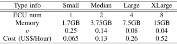
We present an evaluation for our provisioning algorithm. We simulate job sets based on real world trace result in [15], which is measured from Facebook. Because the trace result does not contain job type information, we randomly choose job type from Wordcount and Grep. The sizes of input data follow same distribution of the trace result. In the trace result, 58% of the jobs are small jobs whose input data sizes are smaller than 1.2GB. There are also huge jobs. 3% of the jobs have over 100GB input data. We choose instances from four types of Amazon EC2 instances: Small, Media, Large and XLarge. Their compute capacities, performance degradation ratiosvand hourly cost are shown in Table.I. We used a Small instance to perform as master in the cluster. We assume cluster preparation time t(ip) be in proportional to ni which means
more slave instances cost more preparation time. We sett(ip)= 20ni. We compare our algorithm with cost aware provisioning
algorithm in [16].
Job set and budget are two important inputs for any resource provisioning algorithms. We first evaluate our algorithm under different budgets with fixed job number 100 in the job set. Then we evaluate our algorithm by adjusting job set size with fixed 100US$ budget.
TABLE I: Detail information for different types of instances Type info Small Median Large XLarge
ECU num 1 2 4 8
Memory 1.7GB 3.75GB 7.5GB 15GB
v 0.25 0.14 0.08 0.04
Cost (US$/Hour) 0.065 0.13 0.26 0.52
Current cost model in Amazon is linear, number of ECUs is linear to hourly cost. For a resource provisioning algorithm, cost model greatly affects decisions the algorithm makes. In order to examine effects of different cost model, we evaluate our algorithm under another two cost models: convex and concave. The hourly cost for each type of instance is shown in Table.II. In the convex cost model, per-ECU cost for renting instances increase with ECU number of the instances type, which means that when we are requiring high-end VMs, we pay more for same compute capacity. In the concave cost model, per-ECU cost decreases with instance’s ECU number.
TABLE II: Hourly cost for different types under different cost model (US$) Cost model Small Median Large XLarge
Convex 0.065 0.14 0.29 0.59 Concave 0.065 0.12 0.23 0.45
B. Evaluation Results
In Fig.5, we shows the performance of different algorithms under budget changes. We see that our algorithm outperforms cost-aware algorithm in all cases. Cost-aware algorithm tends to use Small instances because Small instance offers bet-ter provisioning granularity than larger instances. We also notice that the maximum performance difference between interference-aware algorithm and cost-aware algorithm is 11%,
40 60 80 100 120 140 160 8 9 10 11 12 13 14 15 Budget (US$)
Job Completion Time (hour)
Cost aware provisioning Interference aware provisioning
Fig. 5: Job completion time vs bud-get. Job number is 100. Cost model is linear. 0 100 200 300 400 0 20 40 60 80 100 Job number
Job Completion Time (hour)
Cost aware provisioning Interference aware provisioning
Fig. 6: Job completion time vs job number. Budget is 100US$. Cost model is linear. 40 60 80 100 120 140 160 8 9 10 11 12 13 14 15 Budget (US$)
Job Completion Time (hour)
Cost aware provisioning Interference aware provisioning
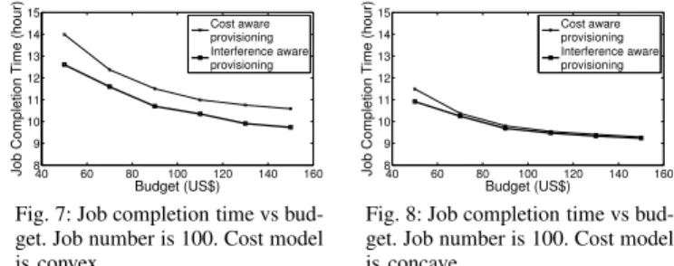
Fig. 7: Job completion time vs bud-get. Job number is 100. Cost model is convex. 40 60 80 100 120 140 160 8 9 10 11 12 13 14 15 Budget (US$)
Job Completion Time (hour)
Cost aware provisioning Interference aware provisioning
Fig. 8: Job completion time vs bud-get. Job number is 100. Cost model is concave.
which is not as much as the performance degradation ratio difference 25%−4% between XLarge instance and Small instance. Because 58% of the jobs is small jobs, in order to suppress over provisioning, our algorithm chooses some Small instance clusters for these jobs. Fig.6 shows comparison of two algorithm with different job number under same budget. We see that there is not obvious difference between interference-aware algorithm and cost-interference-aware algorithm when job number is small because there is enough budget and all jobs can be processed on large clusters. When job number increases, budget becomes limited. Total job completion time increases with job number. Note that, total job completion time does not increase linearly with job number. Because in order to finish all jobs within the budget, both algorithms choose less instances to construct clusters. Thus average job completion time increases. This situation becomes worst when job number further increases. However, our algorithm always outperforms cost-aware algorithm.
We then study the effect of different cost models. In Fig.7, we see that the gap between two algorithm is smaller than the gap in Fig.5 where cost model is linear. If we take a closer look at Fig.7 and Fig.5, we find performance of cost-aware algorithm does not change in two cost models while performance of interference-aware algorithm decreases. This is because in convex cost model, cost for renting larger instances are increased, interference-aware algorithm has to allocate less instances for clusters in order to finish all jobs within the budget. But cost-aware algorithm always uses Small instances whose cost does not change in two cost models. In Fig.8, we see that performance of two algorithms are close and both algorithms finish all jobs in less time. This is because larger instances is more cost-performance effective, both algorithms tend to employ larger instances. It is worth noting that our algorithm still outperform cost-aware algorithm because it chooses cluster type and numbers more accurately.
VI. CONCLUSION
In this paper, we made an observation that a straightforward application of big data systems on cloud platform faces serious interference problems. This poses challenges amid the increasing popularity of using cloud platform to support big data analytics. We conducted a systematic measurement in real world clouds using benchmark big data applications. We showed that the interference is mainly due to CPU-intensive operations and I/O-intensive operations; both of which are unique, yet common for big data systems. To this end, we
re-modeled the resource provisioning of the VMs of the cloud platforms for big data applications; and we developed resource provisioning algorithms to minimize job completion time for job sets given budget constraints. We systematic evaluated our new resource provisioning algorithms. The results confirmed the effectiveness of our schemes.
ACKNOWLEDGMENTS
J. Liu’s work is supported in part by a Canada NSERC Discovery Grant and a China NSFC Major Program of Inter-national Cooperation Grant (61120106008).
REFERENCES
[1] J. Dean and S. Ghemawat, “Mapreduce: simplified data processing on large clusters,”Commun. ACM, vol. 51, pp. 107–113, Jan. 2008. [2] K. Nigam, A. K. McCallum, S. Thrun, and T. Mitchell, “Text
classifi-cation from labeled and unlabeled documents using em,”Mach. Learn., vol. 39, pp. 103–134, May 2000.
[3] P. Costa, A. Donnelly, A. Rowstron, and G. O’Shea, “Camdoop: exploiting in-network aggregation for big data applications,” in Proc. USENIX NSDI, 2012.
[4] T. Condie, N. Conway, P. Alvaro, J. M. Hellerstein, K. Elmeleegy, and R. Sears, “Mapreduce online,” inProc. USENIX NSDI, 2010. [5] F. Chen, M. Kodialam, and T. Lakshman, “Joint scheduling of processing
and shuffle phases in mapreduce systems,” inProc. IEEE INFOCOM, 2012.
[6] A. Pavlo, E. Paulson, A. Rasin, D. J. Abadi, D. J. DeWitt, S. Madden, and M. Stonebraker, “A comparison of approaches to large-scale data analysis,” inProc. ACM SIGMOD, 2009.
[7] M. Stonebraker, D. Abadi, D. J. DeWitt, S. Madden, E. Paulson, A. Pavlo, and A. Rasin, “Mapreduce and parallel dbmss: friends or foes?,”Commun. ACM, vol. 53, pp. 64–71, Jan. 2010.
[8] D. Jiang, B. C. Ooi, L. Shi, and S. Wu, “The performance of mapreduce: an in-depth study,”PVLDB, vol. 3, pp. 472–483, Sept. 2010. [9] “http://sysbench.sourceforge.net/,” 2012.
[10] G. Wang and T. S. E. Ng, “The impact of virtualization on network performance of amazon ec2 data center,” in Proc. IEEE INFOCOM, 2010.
[11] R. Shea and J. Liu, “Network interface virtualization: challenges and solutions,”Network, IEEE, vol. 26, no. 5, pp. 28 –34, 2012.
[12] L. Cherkasova, D. Gupta, and A. Vahdat, “Comparison of the three cpu schedulers in xen,”SIGMETRICS, vol. 35, no. 2, pp. 42–51, 2007. [13] A. Verma, L. Cherkasova, and R. Campbell, “Aria: automatic resource
inference and allocation for mapreduce environments,” in Proc. ACM ICAC, 2011.
[14] B. Palanisamy, A. Singh, L. Liu, and B. Jain, “Purlieus: locality-aware resource allocation for mapreduce in a cloud,” inProc. ACM SC, 2011. [15] M. Zaharia, D. Borthakur, J. Sarma, K. Elmeleegy, S. Shenker, and I. Stoica, “Job scheduling for multi-user mapreduce clusters,” EECS Department, University of California, Berkeley, Tech. Rep., 2009. [16] U. Sharma, P. Shenoy, S. Sahu, and A. Shaikh, “A cost-aware elasticity