Point-Based Approximate Color Bleeding

Point-Based Approximate Color Bleeding

Pixar Technical Memo #08-01 Pixar Animation Studios

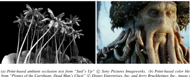
Figure 1: (a) Point-based ambient occlusion test from “Surf ’s Up” cSony Pictures Imageworks. (b) Point-based color bleeding in a final frame from “Pirates of the Carribean: Dead Man’s Chest” cDisney Enterprises, Inc. and Jerry Bruckheimer, Inc., image courtesy of Industrial Light & Magic.

Abstract

This technical memo describes a fast point-based method for com-puting diffuse global illumination (color bleeding). The computa-tion is 4–10 times faster than ray tracing, uses less memory, has no noise, and its run-time does not increase due to displacement-mapped surfaces, complex shaders, or many complex light sources. These properties make the method suitable for movie production. The input to the method is a point cloud (surfel) representation of the directly illuminated geometry in the scene. The surfels in the point cloud are clustered together in an octree, and the power from each cluster is approximated using spherical harmonics. To com-pute the indirect illumination at a receiving point, we add the light from all surfels using three degrees of accuracy: ray tracing, single-disk appoximation, and clustering. Huge point clouds are handled by reading the octree nodes and surfels on demand and caching them. Variations of the method efficiently compute area light il-lumination and soft shadows, final gathering for photon mapping, HDRI environment map illumination, multiple diffuse reflection bounces, ambient occlusion, and glossy reflection.

The method has been used in production of more than a dozen fea-ture films, for example for rendering Davy Jones and his crew in two of the “Pirates of the Caribbean” movies.

Keywords: Global illumination, color bleeding, radiosity, area lights, ambient occlusion, point clouds, point-based rendering, sur-fels, complex scenes, movie production.

1

Introduction

Standard methods for global illumination (such as radiosity [Goral et al. 1984], distribution ray tracing [Ward et al. 1988], and pho-ton mapping [Jensen 1996]) have not been widely used in movie production. This is mostly due to their excessive render times and memory requirements for the very complex scenes that are used in movie production. Not only do the scenes have very complex base

geometry — the light sources, surface and displacement shaders are also very complex and take a long time to evaluate.

In this technical memo we describe a two-pass point-based ap-proach that is much faster and uses less memory than the standard methods. First a surfel representation of the directly illuminated geometry is created in a precomputation phase and stored in a point cloud file. (A surfel is a disk-shaped surface element, i.e. a point with associated normal, radius, and other data such as color. In our case, each surfel represents color reflected from a small part of a surface.) Then the surfels in the point cloud are organized into an octree hierarchy, and the illumination from the surfels in each octree node is approximated using spherical harmonics.

To compute the global illumination at a surface point, we add the illumination from all surfels using three degrees of accuracy: over-lapping surfels are ray traced, other nearby surfels are approximated as disks, and distant surfels are accounted for by evaluating the spherical harmonic representation of clusters. The contributions are sorted according to distance and rasterized onto a coarse cube of “pixels”. Finally, the indirect illumination (color bleeding) is com-puted by multiplying the pixel colors with the BRDF for the chosen reflection model (for example cosine weights for diffuse reflection) and the solid angle of the raster pixels.

Huge point sets are handled efficiently by reading the octree nodes and surfels on demand and caching them.

The advantages of our point-based global illumination method are: faster computation time; the geometric primitives do not have to be kept in memory; no ray-tracing acceleration data structure is needed; only a small fraction of the octree and surfels need to be in memory at any given time; no noise; displacement mapping and complex light source and surface shaders does not slow it down; environment illumination does not take any additional time. The disadvantages are mainly that it is a two-pass approach, and that the results are not guaranteed to be as precise as ray tracing. How-ever, our goal in this project is not numerical accuracy, just visually acceptable and consistent results.

A prototype implementation of the method was immediately adopted for use in movie production at Sony, ILM, and elsewhere. By now the method is built into Pixar’s RenderMan (PRMan) and has been used in the production of more than a dozen feature films1. Figure 1 shows two examples of images computed with the method.

2

Related work

Our algorithm is inspired by the point-based ambient occlusion and color bleeding algorithms of Bunnell [2005], and we use a similar disk approximation for medium-distance points. However, for clus-ters of distant surfels we use a spherical harmonics representation (closely related to clustering methods for finite-element global illu-mination calculations [Smits et al. 1994; Sillion 1995; Christensen et al. 1997]) instead of a single “aggregate” disk, and for very close surfels we use a more precise ray-traced solution. Our resolution of near-vs-far colors is faster and more accurate than Bunnell’s itera-tive approach. We also generalize the algorithm to handle e.g. area light sources, HDRI illumination, and glossy reflection.

The workflow of our algorithm is very similar to the subsurface scattering method of Jensen and Buhler [2002]: the input is a point cloud of surface illumination samples, the point cloud is organized into an octree, power and area values are computed for each oc-tree node, and subsurface scattering or color bleeding is computed at surface points. One difference is that the information stored in the octree nodes is un-directional power and area for subsurface scattering, but spherical harmonics for the directional variation of power and projected area for color bleeding. So even though our algorithm does not compute subsurface scattering, the workflow is very similar.

Our algorithm also has some similarities to hierarchical radios-ity [Hanrahan et al. 1991]. Hierarchical radiosradios-ity is a finite-element solution method that transports light between surface elements at an appropriate level to save time but maintain accuracy. One limitation of hierarchical radiosity is that it only subdivides surfaces patches, but cannot merge them. This limitation was overcome in the face cluster radiosity work by Willmott et al. [1999]. The main simi-larity between these hierarchical radiosity methods and our work is that the light emitters are clustered together to speed up the com-putations. Hierarchical radiosity also clusters the light receivers, which we don’t currently do (although this would be an interesting area of future work).

Dobashi et al. [2004] apply the hierarchical radiosity method to point-sampled geometry. Their method creates a hierarchy of sur-fels, with each cluster containing surfels in the same region of space and with similar normals. Radiosity is transported between clusters of surfels where possible, and between individual surfels when nec-essary to obtain the required accuracy. Their method can also add additional receiving points in areas where the illumination needs to be represented more accurately than the original point density al-lows. The main difference between their method and ours is that they use ray tracing of the surfel disks to determine visibility be-tween surfels, while we use rasterization.

The first successful application of global illumination in a feature-length movie was for the movie “Shrek 2” [Tabellion and Lam-orlette 2004]. They computed direct illumination and stored it as 2D texture maps on the surfaces, and then used distribution ray

1_{“Pirates of the Caribbean: Dead Man’s Chest”, “Eragon”, “Surf’s Up”,}

“Spiderman 3”, “Pirates of the Caribbean: At World’s End”, “Harry Potter and the Order of the Phoenix”, “The Cronicles of Narnia”, “10,000 BC”, “Fred Claus”, “Batman: The Dark Knight”, “Beowulf”, “The Spiderwick Chronicles”, and “Wall-E”.

tracing against a coarsely tessellated version of the scene to com-pute single-bounce color bleeding. The use of 2D textures re-quires the surfaces to have a parameterization. The irradiance at-las method [Christensen and Batali 2004] is similar, but since it uses 3D texture maps (“brick maps”) the surfaces do not need a 2D parameterization. We show in the following that our point-based method is faster and uses less memory than such ray-traced meth-ods.

The interactive global illumination method of Wald et al. [2003] uses distribution ray tracing on a cluster of PCs to compute fast, but coarse global illumination images. The goal of that system was not movie-quality images, and the system only uses very simple shaders and no displacement.

M´endez Feliu et al. [2003] introduced a fast short-range ray-traced approximation that uses the raw object color for color bleeding. It is a nice hybrid approach that gets some color bleeding effects with no additional cost over ambient occlusion. But since it does not take illumination and textures into account, it is too coarse an appromixation for the effects we are trying to obtain here. Haˇsan et al. [2006] presented an interactive system for global illu-mination. Their system represents the scene as a point cloud and precomputes the influence of each point on all other points (and stores this information in a clever compressed format). During an interactive session, the user can change illumination and surface shaders, and the global illumination is automatically updated. Un-fortunately the precomputation is quite lengthy (several hours for realistically complex scenes). In contrast, our goal is to compute the global illumination just once, but as fast as possible, so a long precomputation is not desirable.

In subsequent work [Haˇsan et al. 2007], the same authors did away with most of the precomputation. Instead they represent the illu-mination in the scene as around 100,000 point lights, sample and analyze the transport matrix, and render the most important rows and columns using a GPU.

The method of Meyer and Anderson [2006] computes a sequence of noisy ray-traced global illumination images and filters them to remove the noise. Our method produces noise-free images fast, so there is no need for noise reduction. Also, since our method com-putes one image at a time, we believe it fits better into the traditional movie production pipeline.

In recent work, Lehtinen et al. [2008] use meshless hierarchical ba-sis functions based on illumination samples at surface points. The light is transported between a hierarchy of points (similar to the hi-erarchy we use to represent light emitters), but the actual transfer coefficients between groups of points is computed using ray trac-ing against the original surfaces. In other words, their method is a hybrid point-and-geometry method, while ours uses only points. An early version of the method presented in in this memo was de-scribed in the book “Point-Based Graphics” [Christensen 2007]. Since then, we have improved the method with caching for re-duced memory use, ray-tracing of nearby points for improved ac-curacy, and color sorting for better resolution of near-vs-far colors and deeper shadows.

3

Point-based color bleeding

The input to the method is a point cloud of surfels with direct il-lumination values. The method first organizes the surfels into an octree and computes data for each octree node. Then, for each re-ceiving point, the octree is traversed, the color contributions of sur-fels and clusters are rasterized, and the color bleeding is computed

as a weighted sum of the rasterized pixels. This section describes each step in detail.

3.1 Input: a direct illumination point cloud

The input is a point cloud of surfels (direct illumination sam-ple points). In our imsam-plementation, we use a REYES-type ren-derer [Cook et al. 1987] to subdivide the surfaces into small microp-olygons, compute the color of each micropolygon, and store the colored micropolygons as surfels. Computing the color of the mi-cropolygons requires evaluation of the direct illumination (poten-tially from many light sources), surface shaders (including texture map lookups, procedural shading, etc.), and frequently displace-ment shaders. This step is often referred to as “baking the direct illumination” in TD terminology. Figure 2(a) shows the direct il-lumination point cloud for a simple scene, and figure 2(b) shows a close-up where the size of the disk-shaped surfel represented by each point is visible.

Figure 2: Direct illumination point cloud for a simple scene:

(a) Points. (b) Close-up showing surfels.

To generate the point cloud representation, the camera must be pulled back or the viewing frustum enlarged so that all the parts of the scene that should contribute color bleeding are within view. In the example above, distant parts of the ground plane are not in-cluded in the point cloud, so no color will bleed from those parts of the ground plane. Rendering parameters must be set to ensure that surfaces that face away from the camera or are hidden behind other surfaces are shaded; otherwise those surfels will be missing. The user is free to adjust the tessellation rate and hence the number of points in the point cloud (the accuracy of the surfel representa-tion) — the point cloud does not need to have exactly one surfel for each receiving point in the final image. The user can also use other techniques to generate the point cloud, if desired.

One slightly confusing detail is that we compute two different rep-resentations of the size of each surfel. Each point needs a disk radius that circumscribes the micropolygon that it represents; this is to ensure that the surfaces are completely covered by the surfels with no gaps in between. This radius obviously represents an area that is larger than the real area of the surfel, and if we used it for light transport there would be too much color bleeding from each surfel. So we store the exact area of the surfel in addition to the circumscribing radius.

3.2 Building an octree and computing spherical har-monics

First, the surfels in the point cloud are organized into an octree. The octree nodes are split recursively until each node contains a small number of surfels, for example less than 16.

Then we compute a spherical harmonic representation of the power emitted from (as well as the projected area of) the surfels in each octree node.

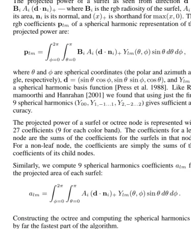
The projected power of a surfel as seen from direction d is

BiAi(d·ni)+— whereBiis the rgb radiosity of the surfel,Aiis its area,niis its normal, and(x)+is shorthand formax(x,0). The rgb coefficientsplm of a spherical harmonic representation of the projected power are:

plm= Z 2π φ=0 Z π θ=0 BiAi(d·ni)+Ylm(θ, φ) sinθ dθ dφ ,

whereθandφare spherical coordinates (the polar and azimuth an-gle, respectively),d= (sinθ cosφ,sinθ sinφ,cosθ), andYlmis a spherical harmonic basis function [Press et al. 1988]. Like Ra-mamoorthi and Hanrahan [2001] we found that using just the first 9 spherical harmonics (Y00, Y1,−1...1, Y2,−2...2) gives sufficient

ac-curacy.

The projected power of a surfel or octree node is represented with 27 coefficients (9 for each color band). The coefficients for a leaf node are the sums of the coefficients for the surfels in that node. For a non-leaf node, the coefficients are simply the sums of the coefficients of its child nodes.

Similarly, we compute 9 spherical harmonics coefficientsalmfor the projected area of each surfel:

alm= Z 2π φ=0 Z π θ=0 Ai(d·ni)+Ylm(θ, φ) sinθ dθ dφ .

Constructing the octree and computing the spherical harmonics is by far the fastest part of the algorithm.

3.3 Octree traversal

To compute the color bleeding at a point we traverse the octree and rasterize the illumination from each surfel and cluster of surfels. The solid angle of each cluster is used to determine whether it or its children should be used. Here is a pseudo-code listing of the octree node traversal algorithm:

traverseOctree(node, maxsolidangle, pos): if (node is a leaf) {

for each surfel in node

rasterize surfel as a disk or ray trace; } else { // node is a cluster of points

if (node bounding box is below horizon) return; evaluate spherical harmonics for cluster area; solidangle = cluster area / distanceˆ2; if (solidangle < maxsolidangle) { // cluster ok

evaluate spherical harmonics for cluster power; rasterize the cluster as a disk;

} else { // recurse for each child node

traverseOctree(child, maxsolidangle, pos); }

}

3.4 Rasterization

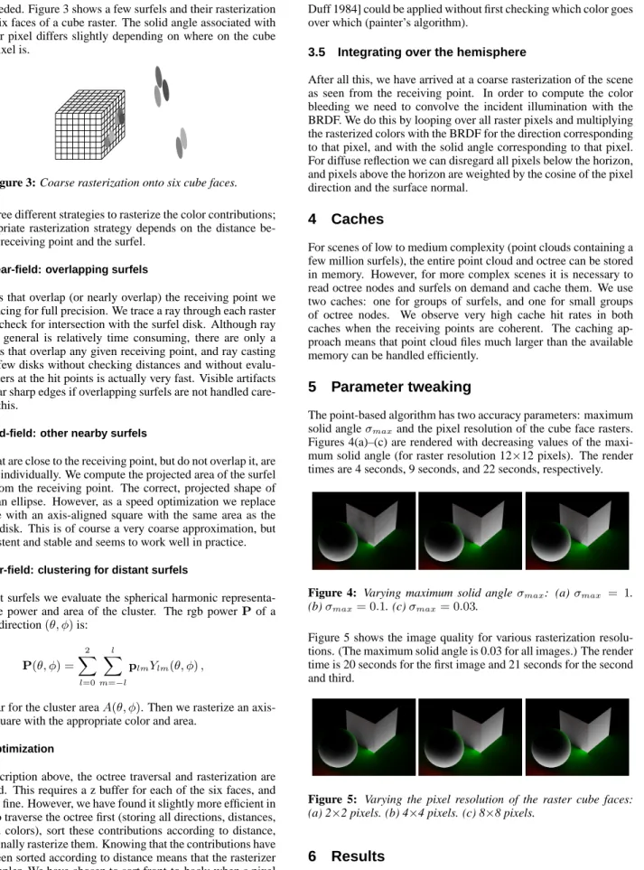
In all but the simplest scenes, too much color bleeding will result if the contributions from all surfels and clusters are simply added to-gether. Instead, we need to ensure that objects hidden behind other objects do not contribute. To do this, we compute a coarse raster-ization of the scene as seen from each receiving point. One way to think of this is as a low-resolution fish-eye image of the scene as seen from each receiving point. In our first implementation we used a hemispherical raster (oriented according to the surface normal), but rasterizing onto a hemisphere requires square roots, sines, and cosines. With an axis-aligned cube raster these expensive functions

are not needed. Figure 3 shows a few surfels and their rasterization onto the six faces of a cube raster. The solid angle associated with each raster pixel differs slightly depending on where on the cube face the pixel is.

Figure 3: Coarse rasterization onto six cube faces.

We use three different strategies to rasterize the color contributions; the appropriate rasterization strategy depends on the distance be-tween the receiving point and the surfel.

3.4.1 Near-field: overlapping surfels

For surfels that overlap (or nearly overlap) the receiving point we use ray tracing for full precision. We trace a ray through each raster pixel and check for intersection with the surfel disk. Although ray tracing in general is relatively time consuming, there are only a few surfels that overlap any given receiving point, and ray casting against a few disks without checking distances and without evalu-ating shaders at the hit points is actually very fast. Visible artifacts appear near sharp edges if overlapping surfels are not handled care-fully like this.

3.4.2 Mid-field: other nearby surfels

Surfels that are close to the receiving point, but do not overlap it, are rasterized individually. We compute the projected area of the surfel as seen from the receiving point. The correct, projected shape of a disk is an ellipse. However, as a speed optimization we replace the ellipse with an axis-aligned square with the same area as the projected disk. This is of course a very coarse approximation, but it is consistent and stable and seems to work well in practice. 3.4.3 Far-field: clustering for distant surfels

For distant surfels we evaluate the spherical harmonic representa-tion of the power and area of the cluster. The rgb powerPof a cluster in direction(θ, φ)is:

P(θ, φ) = 2 X l=0 l X m=−l plmYlm(θ, φ),

and similar for the cluster areaA(θ, φ). Then we rasterize an axis-aligned square with the appropriate color and area.

3.4.4 Optimization

In the description above, the octree traversal and rasterization are interleaved. This requires a z buffer for each of the six faces, and works just fine. However, we have found it slightly more efficient in practice to traverse the octree first (storing all directions, distances, areas, and colors), sort these contributions according to distance, and then finally rasterize them. Knowing that the contributions have already been sorted according to distance means that the rasterizer can be simpler. We have chosen to sort front-to-back; when a pixel is fully covered no further color is added to it. Alternatively, the sorting could be back-to-front, and the “over” operator [Porter and

Duff 1984] could be applied without first checking which color goes over which (painter’s algorithm).

3.5 Integrating over the hemisphere

After all this, we have arrived at a coarse rasterization of the scene as seen from the receiving point. In order to compute the color bleeding we need to convolve the incident illumination with the BRDF. We do this by looping over all raster pixels and multiplying the rasterized colors with the BRDF for the direction corresponding to that pixel, and with the solid angle corresponding to that pixel. For diffuse reflection we can disregard all pixels below the horizon, and pixels above the horizon are weighted by the cosine of the pixel direction and the surface normal.

4

Caches

For scenes of low to medium complexity (point clouds containing a few million surfels), the entire point cloud and octree can be stored in memory. However, for more complex scenes it is necessary to read octree nodes and surfels on demand and cache them. We use two caches: one for groups of surfels, and one for small groups of octree nodes. We observe very high cache hit rates in both caches when the receiving points are coherent. The caching ap-proach means that point cloud files much larger than the available memory can be handled efficiently.

5

Parameter tweaking

The point-based algorithm has two accuracy parameters: maximum solid angleσmaxand the pixel resolution of the cube face rasters. Figures 4(a)–(c) are rendered with decreasing values of the maxi-mum solid angle (for raster resolution 12×12 pixels). The render times are 4 seconds, 9 seconds, and 22 seconds, respectively.

Figure 4: Varying maximum solid angleσmax: (a)σmax = 1. (b)σmax= 0.1. (c)σmax= 0.03.

Figure 5 shows the image quality for various rasterization resolu-tions. (The maximum solid angle is 0.03 for all images.) The render time is 20 seconds for the first image and 21 seconds for the second and third.

Figure 5: Varying the pixel resolution of the raster cube faces:

(a) 2×2 pixels. (b) 4×4 pixels. (c) 8×8 pixels.

6

Results

Figure 6 shows color bleeding in a scene with a car consisting of 2155 NURBS patches (many of which have trimming curves). The

images are 1024 pixels wide and are rendered on a 2.66 GHz Apple Mac G5 computer with four cores and 4 GB memory. Figure 6(a) is rendered with ray tracing and irradiance interpolation [Ward and Heckbert 1992]. It is computed with 730 rays/pixel on average, and took 31.5 minutes to render. Figure 6(b) shows a point-based solution computed with 4.1 million surfels and a maximum solid angle of 0.02. It takes 5.5 minutes to render this image (including 18 seconds to construct the octree and compute spherical harmon-ics). So for this scene the point-based solution is roughly 5.7 times faster than ray tracing for visually similar results. The memory use is 632 MB for ray tracing and 420 MB for the point-based image.

Figure 6: Color bleeding on a NURBS car and ground plane.

(a) Ray-traced image. (b) Point-based image.

Figure 1(a) shows an early ambient occlusion test from the Sony movie “Surf’s Up”. The geometry of the palm trees is so complex that PRMan needs 7.2 GB to ray trace this scene — more than the memory available on a standard PC or renderfarm blade. (Our ray-tracing implementation keeps all high-level geometry in memory; 3.4 GB of very dense subdivision meshes in this case.) But with the point-based method, rendering the scene uses only 828 MB (includ-ing 7.9 million surfels in the point cloud) and easily fits in memory. Figure 1(b) shows Davy Jones in a final frame from the movie “Pi-rates of the Carribean: Dead Man’s Chest”. This image was ren-dered by ILM using our point-based color bleeding method. It is unfortunately hard to know exactly which component of this com-plex image is color bleeding, but the lead R&D engineer at ILM re-ported that the point-based approach was three to four times faster than a noisy ray-traced result for scenes like this one [Hery 2006].

7

Special cases and extensions

This section provides an overview of several useful variations of the point-based color bleeding method. All images are 1024 pixels wide unless otherwise indicated.

7.1 Area light sources and soft shadows

Diffuse area light sources can be handled by simply treating them as bright surfaces. With this approach, the area lights can have arbitrary shapes and color variations across their surface — just as surfaces can. The only requirement is that a point cloud must be generated for the light sources and shadow casters.

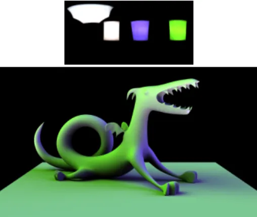
Figure 7 shows a scene with three area light sources: a teapot, a sphere, and a dragon. The teapot light source has a procedu-ral checkerboard texture, the sphere light source is displacement-mapped and displacement-mapped, and the dragon light source is texture-mapped as well. The area lights illuminate three objects: a dragon, a sphere, and the ground plane. Note the correct soft shadows on the ground plane. (To avoid over-saturation that makes the textures hard to see, the light source objects are rendered dimmer than the intensity used for baking their emission.)

Figure 7: Point-based area lights.

7.2 Final gathering for photon mapping

Another application of this method is for photon mapping [Jensen 1996] with precomputed radiance and area estimates [Christensen 1999]. The most time-consuming part of photon mapping is the ray-traced final gathering step needed to compute high-quality im-ages. The point-based color bleeding method presented here can be used directly to speed up the final gathering step. In this applica-tion, the points in the point cloud represent coarse global illumina-tion computed with the photon mapping method (instead of direct illumination).

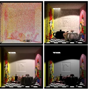
Figure 8 shows a textured box with two teapots (one specular and one displacement-mapped diffuse). Figure 8(a) is the photon map for this scene, with the photon powers shown. The photon map contains 2.6 million photons and took 63 seconds to generate. Fig-ure 8(b) shows the radiance estimates at the photon positions. The estimates were computed from 200 photons each, and took 97 sec-onds to compute. Figure 8(c) is the final image, where point-based color bleeding was used instead of the usual ray-traced final gath-ering. (The reflections in the chrome teapot were computed with ray tracing.) This image took 54 seconds to render (at 400×400 pixel resolution). Figure 8(d) shows the direct illumination alone for comparison.

Figure 8: Textured box with displacement-mapped teapots: (a) Photon map. (b) Radiance estimates. (c) Point-based color bleeding. (d) Direct illumination only.

7.3 Environment illumination

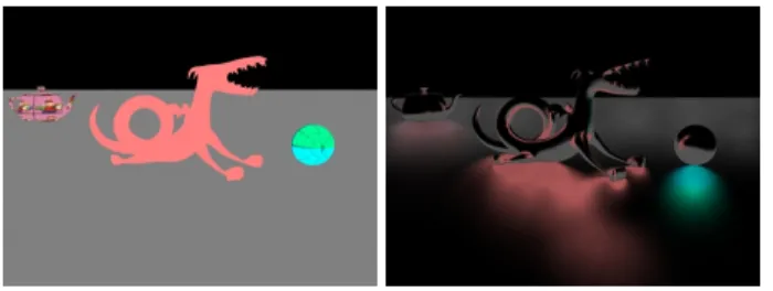
Environment illumination from a standard or high-dynamic range image is easily added to the method. First a filtered environment map lookup is done for each direction and cone angle correspond-ing to a raster pixel. With the axis-aligned cube rasterization ap-proach, this can be done once and for all for each environment map, so comes at neglible run-time cost. Then, during the rasterization for each receiving point, the rasterization simply renders disk colors “over” the environment map colors. The result is that the environ-ment illuminates the receiving points from the directions that are unblocked by geometry. Figure 9(a) shows an HDRI environment map with four areas of bright illumination: two white, one green, and one blue), and figure 9(b) shows a dragon scene illuminated by the environment map. The image took 2.2 minutes to compute.

Figure 9: Point-based environment illumination: (a) HDRI

envi-ronment map (dimmed for display). (b) Dragon illuminated by en-vironment map.

Note that this method will blur high frequencies in the environment map. With our raster resolution of 12×12 pixel per cube face, the finest details in the environment map that can be represented are approximately4π/(6×12×12)≈0.015steradian.

7.4 Multiple bounces

A simple extension allows the method to compute multiple bounces of diffuse reflection. For this variation, it is necessary to store sur-face reflection coefficients (diffuse color) along with the radiosity and area of each surfel. Then we can simply iterate the algorithm, updating the radiosity of the surfels in the point cloud in each iter-ation.

Figure 10 shows a comparison of 0, 1, and 2 bounces in a Cor-nell box scene. The indirect illumination gets brighter with more bounces.

Figure 10: Cornell box with spheres: (a) Direct illumination.

(b) 1 bounce. (c) 2 bounces.

7.5 Ambient occlusion

Ambient occlusion [Zhukov et al. 1998; Landis 2002] is a represen-tation of how much of the hemisphere above each point is covered by geometry. Ambient occlusion is widely used in movie produc-tion since it is relatively fast to compute and gives an intuitive indi-cation of curvature and spatial relationships. It is usually computed with ray tracing: a number of rays are shot from each receiving point, sampling the “coverage” above that point.

Point-based ambient occlusion is a simplified version of the point-based color bleeding algorithm. There is no need to store radiosity in the point cloud; only the point areas are needed. In the rasteri-zation phase, only the alpha channel is used. Also, there is no need to sort according to distance since near-vs-far does not matter for occlusion.

It is common to compute occlusion from both sides of each sur-fel. In this case the 9 spherical harmonics coefficients should be computed using the absolute value ofd·ni:

alm= Z 2π φ=0 Z π θ=0 Ai|d·ni|Ylm(θ, φ) sinθ dθ dφ .

(The three coefficients withl= 1will always be 0 due to the sym-metry of the absolute dot product and the asymsym-metry of those spher-ical harmonics.)

Figure 11 shows point-based ambient occlusion on the car from fig-ure 6. The point cloud used for the computation contains 6.6 million surfels. The image took 3.4 minutes to compute.

Figure 11: Point-based ambient occlusion

7.6 Glossy reflection

The point-based approach can also be used to compute glossy re-flections. For this variation, we collect illumination from a cone of directions centered around the main reflection direction (instead of a hemisphere of directions centered around the surface normal). When traversing the octree, clusters and points outside the cone can be rejected. After rasterization, we multiply the glossy BRDF with the color of the rasterized pixels within the cone. Figure 12 shows an example of point-based glossy reflection.

We use the same six raster faces as for diffuse reflection and ig-nore the raster pixels outside the cone. This means that the glossy coneangle can not be too narrow: for the 12×12 resolution of the raster cube faces, we have found a coneangle of 0.2 radians to be the smallest that gives artifact-free results. For narrower reflection we would recommend using ray tracing. Alternatively, one could use a rasterization onto a single raster covering the directions within the cone. This would avoid wasting raster pixels for directions outside the cone, but is slower since it involves more trigonometric func-tions.

Figure 12: Glossy reflection: (a) Radiosity values in point cloud.

(b) Point-based glossy reflection.

7.7 Irradiance gradients and interpolation

Irradiance interpolation with irradiance gradients [Ward and Heck-bert 1992; Tabellion and Lamorlette 2004] is a very useful tech-nique to speed up ray-tracing based global illumination calcula-tions. We have also implemented irradiance interpolation with irra-diance gradients within our point-based color bleeding algorithm. However, since the point-based irradiance computations are so fast, the gradient computation actually became a bottleneck. In practice we have found that a simpler bilinear interpolation without gradi-ents is preferable for point-based calculations.

7.8 Stand-alone program

As mentioned earlier, we have implemented this point-based algo-rithm (and the variations described above) in Pixar’s RenderMan renderer. We have also implemented our method as a stand-alone program called ptfilter. In this variation, the color bleeding (or am-bient occlusion) is computed at all point positions in a point cloud — either the same point cloud providing the direct illumination and areas, or a separate point cloud providing receiving positions. The advantage of doing the computations in a stand-alone program is that the computation does not use time and memory during render-ing, and that the results can be reused in many re-renderings of the image.

8

Error analysis

The method is only approximate. Here are some of the major sources of error:

• Parts of the scene not included in the direct illumination point cloud will not contribute color bleeding.

• Spherical harmonics truncation: Ramamoorthi and Hanra-han [2001] reported a maximum error of 9% and an aver-age error of 3% when representing environment maps with 9 spherical harmonics. These percentages may seem alarm-ing, however, the error is smooth since the spherical harmon-ics are smooth and the cosines are smooth.

• Clustering error: the approximation of many surfels as a single point with a spherical harmonic distribution is rather coarse. The error introduced by this can be evaluated by set-ting the maximum solid angleσmaxin the algorithm to 0 such that all color bleeding is computed from surfels rather than clusters. We have found that all clusters combined give less than 2% error for typical values ofσmax.

• Discontinuities: there are potentially discontinuities be-tween neighboring receiving points when the octree traversal switches between different representations (two different lev-els in the octree or spherical harmonics vs. individual surflev-els).

We initially experimented with a smooth blend between lev-els, but found that it is not necessary. The reason is that each cluster contributes a rather small fraction of the total color bleeding, so even when one cluster is substituted with finer clusters or a collection of surfels, the change in overall color bleeding is not noticeable.

• Rasterization error: projecting the scene onto six cube faces with 12×12 pixels is of course a rather coarse approximation. Comparing figures 4(c) and 5(c) shows that the visual change when going from 8×8 pixels to 12×12 pixels is minimal. Go-ing to higher resolution gives even less improvement.

• Tiny pieces of geometry that should be “hidden” by other tiny geometry can incorrectly contribute to the color bleeding. This limitation is illustrated (in 2D) in figure 13. The result is that the computed color bleeding will be too strong. (A stochastic ray tracer would get a correct, although noisy, re-sult.) This error can be reduced by increasing the raster cube resolution, but we have not found this necessary for the scenes that are typical in movie production. Note that this problem only occurs if the geometry is sparse; there is no problem if the points together cover the raster pixels.

Figure 13: Geometry giving incorrect color bleeding.

9

Discussion and future work

To be fair to ray tracing, we should mention that our current ray-tracing implementation keeps all high-level geometry in memory. (Surface patches are tessellated on demand and the tessellations kept in a fixed-size LRU cache.) For complex scenes the high-level geometry itself can use more than the available memory. For scan-line rendering (or ray tracing of only camera rays) the memory use is much less since only a very small part of the geometry is needed at any given time, and the geometry can be discarded as soon as it has been rendered. For ray-traced indirect illumination or ambient occlusion, however, the rays can have very incoherent patterns and all high-level geometry needs to be kept in memory.

When comparing render times with ray tracing, one should keep in mind that the best case for ray tracing is simple scenes with a few large spheres and polygons with smooth color, while the worst case for ray tracing is complex scenes with many trimmed NURBS patches, subdivision surfaces with intricate base meshes, displace-ment mapping, etc., and high-frequency textures and shadows. Most of our implementation is multithreaded: several threads can traverse the octree and rasterize independently of each other. The one remaining part that is not yet multithreaded is the octree con-struction; we leave this as future work.

We have implemented multiple diffuse bounces and single glossy reflection, but not multiple glossy reflections. This would proba-bly require the results of the intermediate bounces to be stored as spherical harmonic coefficients at each point.

It would be interesting to utilize SIMD instructions (SSE/Altivec) to speed up the implementation. For example, we could probably

rasterize several pixels covered by one surfel or cluster simultane-ously.

It would also be interesting to investigate a possible GPU imple-mentation of this method. Bunnell’s point-based algorithm was im-plemented on a GPU, so it may be possible to port the extensions and improvements described in this paper back to the GPU.

10

Conclusion

We have presented a fast point-based method for computation of color bleeding, area light illumination, final gathering, HDRI envi-ronment map illumination, multiple diffuse bounces, ambient oc-clusion, and glossy reflection. The method is significantly faster and more memory efficient than previous methods, and was im-mediately adopted for use in movie production at Sony, ILM, and elsewhere.

Acknowledgements

Thanks to Dana Batali and my colleagues in Pixar’s RenderMan Products group for their help in this project.

Thanks to Rene Limberger and Alan Davidson at Sony Imageworks who prompted the start of this project and tested early prototypes, and to Christophe Hery at ILM who was brave enough (or perhaps had the foolhardy guts) to push this techique into movie production while the code was still not quite stable.

Also thanks to Max Planck, Chris King, Carl Frederick and others for testing at Pixar, and to Mark Meyer for helpful comments.

References

BUNNELL, M. 2005. Dynamic ambient occlusion and indirect

lighting. In GPU Gems 2, M. Pharr, Ed. Addison-Wesley Pub-lishers, 223–233.

CHRISTENSEN, P. H., AND BATALI, D. 2004. An irradiance

atlas for global illumination in complex production scenes. In Rendering Techniques 2004 (Proc. Eurographics Symposium on Rendering), 133–141.

CHRISTENSEN, P. H., LISCHINSKI, D., STOLLNITZ, E. J.,AND SALESIN, D. H. 1997. Clustering for glossy global illumination. ACM Transactions on Graphics 16, 1, 3–33.

CHRISTENSEN, P. H. 1999. Faster photon map global illumination. Journal of Graphics Tools 4, 3, 1–10.

CHRISTENSEN, P. H. 2007. Point clouds and brick maps for movie production. In Point-Based Graphics, M. Gross and H. Pfister, Eds. Morgan Kaufmann Publishers, ch. 8.4.

COOK, R. L., CARPENTER, L.,ANDCATMULL, E. 1987. The Reyes image rendering architecture. Computer Graphics (Proc. SIGGRAPH 87) 21, 4, 95–102.

DOBASHI, Y., YAMAMOTO, T.,ANDNISHITA, T. 2004. Radiosity for point-sampled geometry. In Proc. Pacific Graphics 2004, 152–159.

GORAL, C. M., TORRANCE, K. E., GREENBERG, D. P., AND BATAILLE, B. 1984. Modeling the interaction of light between diffuse surfaces. Computer Graphics (Proc. SIGGRAPH 84) 18, 3, 213–222.

HANRAHAN, P., SALZMAN, D., AND AUPPERLE, L. 1991.

A rapid hierarchical radiosity algorithm. Computer Graphics (Proc. SIGGRAPH 91) 25, 4, 197–206.

HASANˇ , M., PELLACINI, F.,ANDBALA, K. 2006. Direct-to-indirect transfer for cinematic relighting. ACM Transactions on Graphics (Proc. SIGGRAPH 2006) 25, 3, 1089–1097.

HASANˇ , M., PELLACINI, F.,ANDBALA, K. 2007. Matrix row-column sampling for the many-light problem. ACM Transactions on Graphics (Proc. SIGGRAPH 2007) 26, 3, 26.

HERY, C. 2006. Shades of Davy Jones. Interview available at http://features.cgsociety.org/story custom.php?story id=3889. JENSEN, H. W., AND BUHLER, J. 2002. A rapid hierarchical

rendering technique for translucent materials. ACM Transactions on Graphics (Proc. SIGGRAPH 2002) 21, 3, 576–581.

JENSEN, H. W. 1996. Global illumination using photon maps. In Rendering Techniques ’96 (Proc. 7th Eurographics Workshop on Rendering), 21–30.

LANDIS, H. 2002. Production-ready global illumination. In SIG-GRAPH 2002 Course Note #16: RenderMan in Production, 87– 102.

LEHTINEN, J., ZWICKER, M., TURQUIN, E., KONTKANEN, J., DURAND, F., SILLION, F. X.,ANDAILA, T. 2008. A meshless hierarchical representation for light transport. ACM Transactions on Graphics (Proc. SIGGRAPH 2008) 27, 3. To appear. M ´ENDEZFELIU, `A., SBERT, M.,ANDCATA´, J. 2003. Real-time

obscurances with color bleeding. In Proc. Spring Conference on Computer Graphics, 171–176.

MEYER, M.,ANDANDERSON, J. 2006. Statistical acceleration for animated global illumination. ACM Transactions on Graphics (Proc. SIGGRAPH 2006) 25, 3, 1075–1080.

PORTER, T., ANDDUFF, T. 1984. Compositing digital images. Computer Graphics (Proc. SIGGRAPH 84) 18, 3, 253–259. PRESS, W. H., TEUKOLSKY, S. A., VETTERLING, W. T.,AND

FLANNERY, B. P. 1988. Numerical Recipes in C: The Art of Scientific Computing, 2nd ed. Cambridge University Press.

RAMAMOORTHI, R., AND HANRAHAN, P. 2001. An efficient

representation for irradiance maps. Computer Graphics (Proc. SIGGRAPH 2001), 497–500.

SILLION, F. X. 1995. A unified hierarchical algorithm for global illumination with scattering volumes and object clusters. IEEE Transactions on Visualization and Computer Graphics 1, 3, 240– 254.

SMITS, B., ARVO, J., ANDGREENBERG, D. 1994. A cluster-ing algorithm for radiosity in complex environments. Computer Graphics (Proc. SIGGRAPH 94), 435–442.

TABELLION, E., ANDLAMORLETTE, A. 2004. An approximate

global illumination system for computer generated films. ACM Transactions on Graphics (Proc. SIGGRAPH 2004) 23, 3, 469– 476.

WALD, I., BENTHIN, C., ANDSLUSALLEK, P. 2003. Interac-tive global illumination in complex and highly occluded envi-ronments. In Rendering Techniques 2003 (Proc. Eurographics Symposium on Rendering), 74–81.

WARD, G. J.,ANDHECKBERT, P. S. 1992. Irradiance gradients. In Proc. 3rd Eurographics Workshop on Rendering, 85–98. WARD, G. J., RUBINSTEIN, F. M.,ANDCLEAR, R. D. 1988. A

ray tracing solution for diffuse interreflection. Computer Graph-ics (Proc. SIGGRAPH 88) 22, 4, 85–92.

WILLMOTT, A. J., HECKBERT, P. S.,ANDGARLAND, M. 1999. Face cluster radiosity. In Rendering Techniques ’99 (Proc. 10th Eurographics Workshop on Rendering), 293–304.

ZHUKOV, S., IONES, A.,ANDKRONIN, G. 1998. An ambient light illumination model. In Rendering Techniques ’98 (Proc. 9th Eurographics Workshop on Rendering), 45–55.