Fitting generalised linear models to car claims data

Fifth International Conference in Financial and Actuarial Mathematics

Fitting Generalised Linear Models to Car Claims data

Liberato Camilleri, Marianne Cassar

University of Malta,

Department of Statistics and Operations Research [email protected]

Abstract:

Generalised linear models (GLMs) overcome the limitations of Normal regression models since they can accommodate any distribution that is a member of the exponential family. These models allow transformation of the response variable through the canonical link function. This paper presents two GLMs to analyze a data set provided by a car insurance company. The first model is a lognormal regression model that relates claim size to a number of demographic, car-related and policy-related predictors and the second model is a Poisson regression model that relates the number of claims filed by a policy holder to these explanatory variables. An appropriate model that describes the aggregate claim amount in a portfolio of insurance contracts during a fixed period combines both claim size and number of claims through a compound Poisson distribution.

Key words:

Poisson and Lognormal distributions, Iterative reweighted least squares algorithm, Generalized Linear Models, Compound Poisson distribution

Introduction

One of the most far-reaching contributions in statistical modelling is the concept of generalized linear models introduced by John Nelder and Robert Wedderburn (1972). These models relate the response variable to the linear predictor (non-random component) through any invertible link function and accommodate any error distribution that is in the exponential family. Analyzing car claim data using traditional ordinary least squares regression models and ANOVA methods can be problematic. Firstly the distribution of car claim size is very often right skewed and do not follow a Normal distribution; secondly the number of claims made by a policyholder is a discrete variable and would be better accommodated by a discrete distribution. GLMs, on the other hand, provide an integrated conceptual and theoretical framework that can be used to analyze both continuous and categorical response data. Logistic and Probit regression models are appropriate to analyze Binomial response data; whereas Loglinear models are suitable to

analyze Multinomial and Poisson response data. The iteratively re-weighted least squares algorithm that maximizes the log-likelihood function in Generalized Linear models makes use of Fisher scoring. Although GLMs accommodate most of the assumptions of Regression models they still rely on the assumption that the responses are independent.

Estimation

The unity of several statistical methods to analyze response data that departs from the normality assumption was demonstrated by (Nelder and Wedderburn 1972) using the idea of a generalized linear model. This section provides an outline of the properties of GLMs as a comprehensive structure.

Consider a random variable Y whose probability mass function, if it is discrete, _i

or probability density function, if it is continuous is assumed to follow the form of the exponential family of distributions.

(

)

( )

( )

(

)

      + − = = φ φ θ θ , exp _i i i i i i i c y a b y y Y P

It is assumed that the responses Y are independent and identically distributed and _i

the distribution of each Y is a member of the exponential family. Moreover the _i

known values of the explanatory variables influence the distribution of Y through _i

a single linear function or linear predictor η_i

∑

= = p j j ij i x 1 β η

It is also assumed that the mean µ_i =E

( )

Y_i , and linear predictor η_i are related by a smooth invertible link function g

( )

⋅ .

( )

i i g µ

η =

Considering the likelihood L as a function of β, one can find the maximum of L by maximizing 1 log J i i l L =

=

∑

where l_i =logP

(

Y_i = y_i

)

. This is realized by solving the maximum likelihood equations =0

∂ ∂ j i l β for j=1,...,p j i i i i i i i j i η η µ l l β µ θ θ β ∂ ∂ ∂ ∂ ∂ ∂ ∂ ∂ = ∂ ∂

Since

( )

( )

φ

(

φ

)

θ θ , i i i i i i c y a b y l = − + , µ_i =E

( )

Y_i =b'

( )

θ_i and

∑

= = p j j ij i x 1 β η then

( )

( )

( )

φ µ φ θ θ i i i i i i i i a y a b y l − = − = ∂ ∂ ' ,

( )

_i i i _b θ θ µ '' = ∂ ∂ and _ij j i =_x ∂ ∂ β η Moreover, by setting i i i d µ η ∂ ∂ = then

( ) ( )

ij i i i i i j i x d b a y l 1 '' 1 θ φ µ β − = ∂ ∂

Since σ_i2 =var

( )

Y_i =a_i

( ) ( )

φ b'' θ_i then

ij i i i i j i x d y l 2 σ µ β − = ∂ ∂

The log-likelihood function is maximized by solving the equations =0

∂ ∂ j l β for p

j=1,..., . Let U be the scores with respect to parameters j βj such that

j U

∑

∑

(

)

= = − = ∂ ∂ = ∂ ∂ = I i i i ij i i I i j i j d x y l l 1 2 1 σ µ β β

In general the equations U_j =0 for j=1,...,p are non-linear and they have to be solved by numerical iteration. The Newton-Raphson approach to solving these equations would be to set up an iterative scheme for the vector β. The th

m approximation is given by ( ) _ˆ( 1) 1 ( 1) ˆ m ₌ m− ₋ − m− U H β β where       ∂ ∂ ∂ = ' 2 β β

H l is the Hessian matrix evaluated at β=βˆ(m−1) and the score vector (m−1)

U is also evaluated at the previous iteration. These second derivatives are often complicated to calculate. An alternative procedure, which is sometimes simpler than the Newton-Raphson method is called the Fisher scoring technique. It involves replacing the matrix of second derivatives by its matrix of expected values where

(

)

2 2 4 2 1 I ij ik jk i i i j k j k i i x x l l l E E E Y d =  _∂   _{∂ ∂}  Ψ = −  =  = − µ ∂β ∂β ∂β ∂β σ        

∑

Since E

(

Yi −µi

)

2 =var

( )

Yi =σi2 then

∑

− = Ψ I i i i ik ij jk d x x 1 2 2 σ

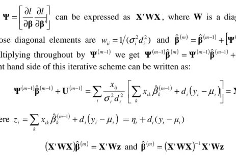
So _      ∂ ∂ ∂ ∂ = ' β β

Ψ l l can be expressed as X'WX, where W is a diagonal matrix

whose diagonal elements are wii=1 (σi2di2) and

( ) _ˆ( 1)

[

( 1)

]

1 ( 1) ˆ m ₌ m− ₊ m− − m− U Ψ β β .

Multiplying throughout by Ψ(m−1) we get Ψ(m−1) ( )βˆ m =Ψ(m−1) (βˆ m−1)+U(m−1). The right hand side of this iterative scheme can be written as:

( −) ( −) ₊ ( −) ₌

∑

i i i ij m m m d x 2 2 1 1 1 _ˆ σ U β Ψ ˆ( 1)

(

)

_=X'Wz      − +

∑

− k i i i m k ik d y x β µ where =

∑

( −)+

(

−

)

k i i i m k ik i x d y z βˆ 1 µ =ηi+d yi( i−µi)

(

)

( ) Wz X β WX X' ˆ m = ' and βˆ( )m =

(

X'WX

)

−1X'Wz

The generalized linear model maximum likelihood estimators are obtained by an iterative weighted least squares procedure.

Application

To implement the theory of GLMs we utilized a data set provided by a local insurance car company, to relate the number of claims filed annually by each policyholder and the claim size made by each claimant to a number of predictors. These explanatory variables included policy-related variables (cover subscription, premium paid annually by policyholder), car-related variables (number of owned cars, engine size) and individual covariates (age of policyholder). Premium paid annually and claim size are continuous variables; number of claims and number of owned cars are discrete variables; whereas cover subscription (Third party only, third party fire and theft, fully comprehensive), engine size (less than 1100, 1100-1500, more than 1500cc) and age of policy holder (18-30, 31-50, more than 50 years) are categorical variables.

The data comprised 9107 policyholders of which 497 made at least one claim. The frequency distribution of claim size, displayed in Figure 1, was considerably right skewed and fitting a Normal regression model to this data was not deemed appropriate. EasyFitXL was used to identify the best contender for the distribution of claim size using the Kolmogorov Smirnov, Anderson Darling and Chi squared criteria. Undoubtedly the Lognormal distribution is identified as the best fitting distribution for claim size.

Distribution

Kolmogorov Smirnov Anderson Darling Chi squared Statistic Rank Statistic Rank Statistic Rank Lognormal 0.0231 1 0.2676 1 4.1677 2

Normal 0.1701 17 26.127 17 131.54 18

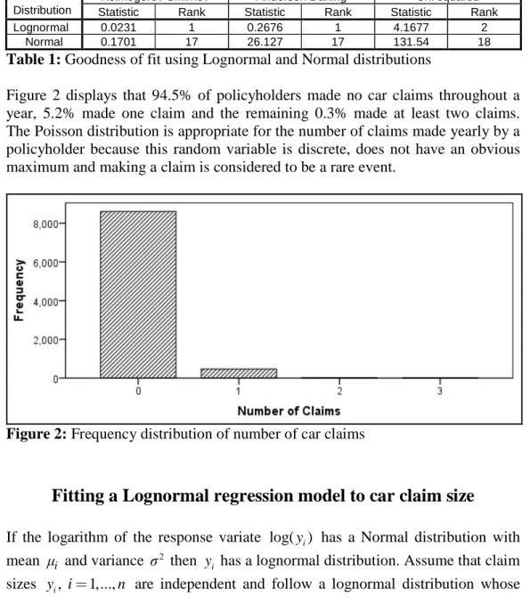
Table 1: Goodness of fit using Lognormal and Normal distributions

Figure 2 displays that 94.5% of policyholders made no car claims throughout a year, 5.2% made one claim and the remaining 0.3% made at least two claims. The Poisson distribution is appropriate for the number of claims made yearly by a policyholder because this random variable is discrete, does not have an obvious maximum and making a claim is considered to be a rare event.

Figure 2: Frequency distribution of number of car claims

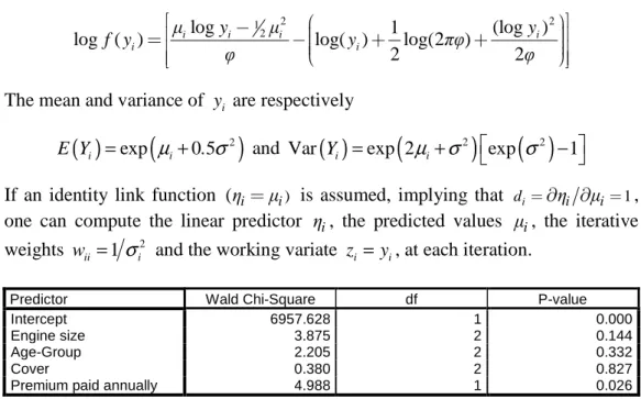
Fitting a Lognormal regression model to car claim size

If the logarithm of the response variate log( )y has a Normal distribution with _i

mean µ_i and variance _σ2 _then

i

y has a lognormal distribution. Assume that claim

sizes yi, i=1,...,n are independent and follow a lognormal distribution whose density function is:

2 2 2 (log ) 1 ( ) exp for 0. 2 2 i i i i i y µ f y y σ y πσ  _  _  _  _       − − = >

This can be expressed as:

2 2

1 2

log 1 (log )

log ( ) log( ) log(2 )

2 2 i i i i i i µ y µ y f y y πφ φ φ  ₋  _   _ =_ −_ + + _       

The mean and variance of y are respectively _i

( )

(

2

)

exp 0 5

i i

E Y = µ + . σ and Var

( )

Y_i =exp 2

(

µ σ_i+ 2

)

_exp

( )

σ2 −1_

If an identity link function (η_i=µ_i) is assumed, implying that d_i=∂η_i ∂µ_i=1, one can compute the linear predictor η_i, the predicted values µ_i, the iterative

weights 2

1 ii i

w = σ and the working variate z_i =y_i, at each iteration.

Predictor Wald Chi-Square df P-value Intercept 6957.628 1 0.000 Engine size 3.875 2 0.144 Age-Group 2.205 2 0.332 Cover 0.380 2 0.827 Premium paid annually 4.988 1 0.026

Table 2: Tests of model effects

The tests of model effects displayed in table 2 indicate that the premium paid annually (in thousands of Euro) is the best predictor of car claim size. This is followed by engine size, age of policyholder and cover subscription. This four-predictor model explain 15.7% of the total variance in the responses indicating that there are other important predictors that contribute significantly in explaining variation in car claim sizes.

Term Parameter Std. Error

95% Wald Confidence Interval Lower Upper Intercept 6.898 0.113 6.676 7.120 Engine size (less than 1100cc) -0.236 0.140 -0.510 0.038 Engine size (1100-1500cc) 0.033 0.099 -0.162 0.229 Engine size (More than 1500cc) 0 . . . Age-Group (18-30 years) 0.254 0.171 -0.081 0.589 Age-Group (31-50 years) 0.047 0.097 -0.144 0.237 Age-Group (More than 50 years) 0 . . . Cover (Third party only) -0.064 0.110 -0.280 0.152 Cover (Third party fire and theft) 0.007 0.130 -0.247 0.262 Cover (Fully comprehensive 0 . . . Premium 0.351 0.157 0.043 0.659 (Scale) 0.830 0.059 0.723 0.953

Table 3: Parameter estimates and corresponding 95% confidence intervals

The parameter estimates, displayed in table 3, reveal interesting contrasts between the levels of the main effects. Policyholders that pay large premiums tend to make bigger claims than other policyholders; young claimants tend to make bigger claims than older ones. Moreover, policyholders possessing small sized engine cars tend to make smaller claims than those possessing large sized engine cars and

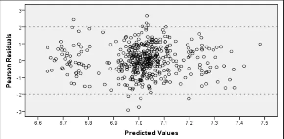
claimants who insure their cars under a third party cover tend to make smaller claims than those who insure their cars under a third party fire and theft or a fully comprehensive cover. The residual plot displayed in Figure 3 exhibits no systematic patterns indicating no model misspecifications. Approximately 95% of all Pearson residuals lie between the ±2 threshold values which conform to what is expected.

Figure 3: Residual plot

Fitting a Poisson regression model to number of claims

Suppose that the response variates yi, i=1,...,n are independent and Poisson distributed y_{i ∼}Poi( )µ_i whose mass function is:

(

)

! i i µ y i i i i e µ P Y y y − = =

The log link is the canonical link function for a random variable having a Poisson distribution η_i=logµ_i, implying that d_i=∂η_i ∂µ_i=1µ_i. Given the fact that the mean and variance of y are both _i µi, one can compute the linear predictor ηi, the

predicted values µ_i, the working variate z_i = +η_i

(

y_i−µ µ_i

)

/ _i and the iterative weights w_ii =µ_i at each iteration.

Predictor Wald Chi-Square df P-value Intercept 2.050 1 0.152 Age-Group 3.094 2 0.213 Cover 47.627 2 0.000 Number of cars owned 15.198 1 0.000 Premium paid annually 6.558 1 0.010

The tests of model effects displayed in table 4 indicate that cover subscription is the best predictor of number of car claims. This is followed by the number of cars owned by policyholder, the premium paid annually (in thousands of Euro) and the age of policyholder. This four-predictor model explain 29.6% of the total variance in the responses indicating that there are other important predictors that contribute significantly in explaining variation in the number of car claims made annually by a policyholder.

Term Parameter Std. Error

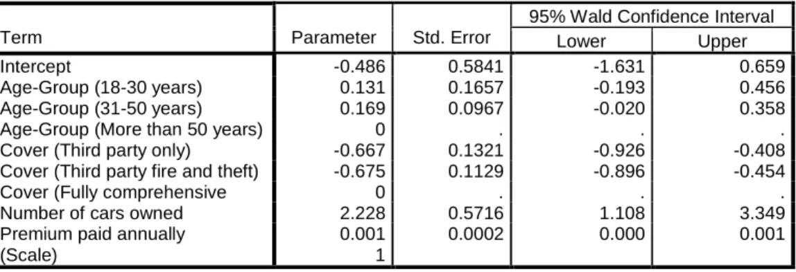
95% Wald Confidence Interval Lower Upper Intercept -0.486 0.5841 -1.631 0.659 Age-Group (18-30 years) 0.131 0.1657 -0.193 0.456 Age-Group (31-50 years) 0.169 0.0967 -0.020 0.358 Age-Group (More than 50 years) 0 . . . Cover (Third party only) -0.667 0.1321 -0.926 -0.408 Cover (Third party fire and theft) -0.675 0.1129 -0.896 -0.454 Cover (Fully comprehensive 0 . . . Number of cars owned 2.228 0.5716 1.108 3.349 Premium paid annually 0.001 0.0002 0.000 0.001 (Scale) 1

Table 5: Parameter estimates and corresponding 95% confidence intervals

The parameter estimates, displayed in table 5, reveal interesting contrasts between the categories of the predictors. Policyholders that pay larger premiums tend to make bigger claims than other policyholders; old claimants tend to make fewer claims than younger ones. Moreover, policyholders who insure their cars under a Fully Comprehensive cover have a tendency to make more claims than others and the number of claims made annually increases with the number of cars owned by the policyholders. Approximately 95% of all Pearson residuals lie between the

2

± threshold values which conform to what is expected.

The compound Poisson distribution

The decomposition of the aggregate claim amount S paid annually by the insurer allows consideration of the number of claims and corresponding claim amounts separately. A practical advantage of this is the factors affecting claim numbers and claim amounts may well be different. For instance, a prolonged spell of bad weather may have a significant effect on claim numbers but little or no effect on the distribution of individual claim amounts. On the other hand, inflation may have a significant effect on the cost of repairing cars, and hence on the distribution of individual claim amounts, but little or no effect on claim numbers. If the random variable N, representing number of claims made by policyholders has a Poisson distribution with parameter λ and X X₁, ₂,...,X are corresponding _N

claim amounts which are assumed independent and identically distributed, then the total claim amount

1 N i i S X =

obtained by marginalizing the joint distribution of ( ,S N over N, which in turn is ) attained by joining the marginal distribution of N with the conditional distribution

S N. If the number of claims N has a Poisson distribution with mean λ and the total claim amount S has a compound Poisson distribution with parameter λ then, [ ] [ ] E N =Var N =λ

( )

( 1) 1 1 ( ) ! ! t t N t n _{tN N λ} n λe tN λ λ λe N N N λe e λ e M t E e e e e e N N − − − − = =             _ _   _{ }   _{ }         = =

∑

=

∑

= =

The expectation of S is obtained by applying the identity [ ]E S =E E S N[ [ | ]]

1 1 [ | ] [ ] n i i E S N n E X nm = = =

∑

= and E S N[ | ]=Nm1 1 1 1 [ ] [ ] [ ] E S =E Nm =E N m =λm

The variance of S is obtained by using Var S[ ]=E Var S N[ [ | ]]+Var E S N[ [ | ]]

2 1 2 1 Var[ | ] [ ] ( ) n i i S N n Var X n m m = = =

∑

= − and Var S N[ | ]=N m( ₂−m₁2) 2 2 2 2 1 1 2 1 1 2 [ ] [ ( )] [ ] ( ) [ ] [ ]

Var S =E N m −m +Var Nm = m −m E N +m Var N =λm

The moment generating function of S is the moment generating function of N evaluated at logM_X( )t .

(

)

( log ( ))

(

)

( ) ( ) N N MX t log ( ) X N X S M t E M t  E e  M M t     _{ }     = = = where M_N( )t =eλ(et−1)

(

)

log ( ) 1 _{( ( ) 1)} ( ) log ( ) M_X t X λe _{λM t} N X S M t M M t e e  _  _        − − = = =

A very important property is that the sum of the independent compound Poisson random variables is itself a compound Poisson random variable. If S1,...,Sn are independent random variables each having a compound Poisson distribution with parameters λ_i and ( ) for F x_i i=1,...,n where F x is the distribution of individual _i( ) claim amounts then

1

n i i

A S

=

=

∑

also has a compound Poisson distribution with parameters 1 Λ=

∑

_in₌ λi ₁ ( ) 1 ( ) Λ n i i i λF x F x =

=

∑

. Table 6 displays the distribution of claim size and the average number of car claims per age group and per cover.

Age Group Distribution of claim size Mean number of claims

18 – 30 years lnN(1277.5, 0.829) λ1 = 0.05108

31 – 50 years lnN(1117.4, 0.963) λ2 = 0.06195

More than 50 years lnN(1039.1, 0.967) λ3 = 0.05334

3

Cover subscription Distribution of claim size Mean number of claims

Third party only lnN(1112.9, 0.895) λ1 = 0.03757

Third party fire and theft lnN(1123.6, 0.871) λ2 = 0.03907

Fully comprehensive lnN(1117.4, 0.942) λ3 = 0.08201

Table 6: Distributions of claim sizes and mean number of claims

Conclusion

The GLMs identified one significant predictor (premium paid annually) for claim size and three significant predictors (cover subscription, number of cars owned, premium paid annually) for number of filed claims. One of the limitations of this study is that the explanatory variables explained a small portion of the variation in the response variables. Indeed other explanatory variables, for instance, speed of car before impact and driving behaviour would have improved predictions if they were recorded.

An alternative approach to address the data heterogeneity is by fitting Latent class models. These models assume that the observed data are actually composed of several homogeneous segments that are mixed together in unknown proportions. The segments are considered latent (unobserved) because the number of clusters and the number of individuals they comprise are unknown. The objective is to estimate the true number of segments and derive a prediction regression model for each segment using the expectation-maximization (EM) algorithm that maximizes the expected log-likelihood function. Indeed the main advantage of using these models over traditional clustering techniques is that estimation and segmentation are carried out simultaneously.

References

:

1. M. Aitkin, D. Anderson, B. Francis, J. Hinde. Statistical Modelling in GLIM, Oxford Science Publications, 1994.

2. A. Dempster, N. Laird, D. Rubin. Maximum Likelihood from Incomplete Data via EM algorithm. Journal of the Royal Statistical Society, 39, 1-38, 1977. 3. P. McCullagh, J. Nelder. Generalized Linear Models, London: Chapman & Hall Publications, 1989.

4. J.A. Nelder, R.W.M. Wedderburn. Generalized Linear Models. Journal of the Royal Statistical Society, A, 135, 370-384, 1972.

5. A. Skrondal, S. Rabe-Hesketh. Generalized Latent Variable Modelling. Chapman & Hall/CRC, 2004.

View publication stats View publication stats