Land Cover Classification using Sentinel-1 Radar Mission Interferometry

Muhammad Arsalan-Ul-Haque

School of Electrical Engineering

Thesis submitted for examination for the degree of Master of Science in Technology.

Espoo 20.08.2017

Thesis supervisor:

Prof. Jaan Praks

Thesis advisor:

Date: 20.08.2017 Language: English Number of pages: 11+69 Department of Electronics and Nanoengineering

Professorship: Space Science and Technology (S-92) Supervisor: Prof. Jaan Praks

Advisor: D.Sc. (Tech.) Oleg Antropov

Synthetic Aperture Radar (SAR) has been widely used for many years in the field of remote sensing. SAR has valuable contribution due to its ability to provide complementary information to optical systems, penetration of radar waves through volumetric targets and high-resolution. SAR has the ability to operate during day and night. It provides operational services under all weather conditions. SAR imagery has many applications including land cover changes, environmental monitoring, climate change and military surveillance.

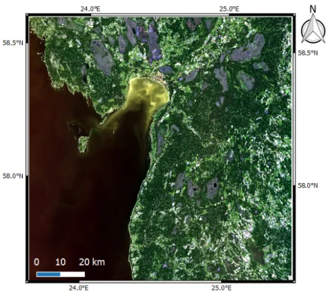
This work focuses on land cover classification with SAR interferometry (InSAR) technique using Sentinel-1 space radar image pair. Sentinel-1 data were collected over the southern part of Estonia. Two SLC SAR images were acquired from both Sentinel-1A and Sentinel-1B with six days temporal difference. In this study, interferometric coherence and backscattering intensity processing chains have been set up and applied to Sentinel-1 SAR image pair. The Sentinel Application Platform (SNAP) has been used for processing of single pair for Sentinel-1 mission. The SNAP is an European Space Agency (ESA) software. The Sentinel-1 image pair processing has been done using Sentinel-1 Toolbox (S1TBX) which is a part of SNAP. Corine Land Cover (CLC) 2012 database has been used as a reference data with 20 m resolution. The CLC2012 contains land use/cover information for most of the European countries. A single optical image from Sentinel-2A was additionally used for feature extraction. An overall accuracy of 68% to 73% was achieved when performing classification into five classes (Urban, Field, Forest,

Peat-land, Water) using supervised classification with k-nearest neighbour (kNN) algorithm. The accuracy assessment was done by using confusion matrices.

Keywords: synthetic aperture radar, SAR, remote sensing, land cover classifica-tion, SAR interferometry, InSAR, interferometric coherence, backscat-tering intensity.

Acknowledgements

The research and report writing has been carried out in the department of Electronics and Nanoengineering of Aalto University over the period of six months from March to August, 2017.

I would first like to express my gratitude to my thesis supervisor Prof. Jaan Praks, Professor in Aalto University, for employing me and giving an opportunity to be part of his research group and carrying out my diploma work under his supervision. He has always been a great support through the learning process and his office door was always opened whenever I had any trouble about research or thesis writing.

Secondly, I want to thank my thesis advisor Dr. Oleg Antropov, Post-Doctoral Researcher in Aalto University, for his guidance and encouragement during the thesis. I am grateful for having him as my advisor and the scientific discussions I had with him were invaluable for the completion of my research work within specified time period.

Finally, I express my gratitude to my parents and friends for being an unfailing support and encouragement throughout my years of study, and especially while making decision to pursue my studies abroad. This achievement would not have been possible without them. Thank you.

Otaniemi, 20.08.2017

Acknowledgements iii

Contents iv

List of Symbols vi

List of Abbreviations vii

1 Introduction 1

1.1 Remote Sensing . . . 2

1.2 InSAR Studies on Land Cover . . . 2

1.3 Motivation . . . 3

1.4 Structure of the Report. . . 3

2 Theoretical Background 4 2.1 Overview of Radar and SAR . . . 4

2.1.1 Principles of Imaging Radar . . . 6

2.1.1.1 Radar System Measurements . . . 7

2.1.1.2 Imaging Radar Frequency Bands . . . 7

2.1.1.3 Microwave Polarizations . . . 7

2.1.1.4 Incidence Angle . . . 8

2.1.2 Radar Backscattering Coefficient . . . 9

2.1.2.1 Parameters Affecting Radar Backscatter . . . 9

2.1.3 Radar Image Geometry. . . 10

2.1.3.1 Viewing Geometry . . . 11

2.1.3.2 Spatial Resolution . . . 12

2.1.3.3 SAR Range Resolution . . . 12

2.1.3.4 SAR Azimuth Resolution . . . 12

2.1.4 SAR Image Types . . . 13

2.1.4.1 Complex Images . . . 13

2.1.4.2 Detected Images . . . 13

2.1.4.3 Single-look Image . . . 13

2.1.4.4 Multi-looked Image. . . 13

2.1.5 Distortions in Radar Images . . . 14

2.1.5.1 Slant-Range Scale Distortions . . . 14

2.1.5.2 Terrain Induced Distortions . . . 14

2.1.6 Radiometric Distortions . . . 15

2.1.7 SAR Processing . . . 16

2.1.7.1 Range Doppler Algorithm (RDA) . . . 17

2.2 InSAR Fundamentals . . . 18

2.2.1.1 Types of SAR Interferometry . . . 19

2.2.1.2 InSAR Baselines . . . 20

2.2.2 Interferometric Phase for Terrain Altitude Measurement . . . 21

2.2.2.1 Interferogram Flattening . . . 22

2.2.2.2 Height of Ambiguity . . . 22

2.2.3 Interferometric Coherence . . . 23

2.3 Land Cover Classification . . . 23

2.3.1 Classification Techniques . . . 24 2.3.1.1 Unsupervised Classification . . . 24 2.3.1.2 Supervised Classification . . . 25 2.3.2 Types of Classifier . . . 26 2.3.2.1 Euclidean Distance . . . 26 2.3.2.2 k-Nearest Neighbour (kNN) . . . 27

2.3.3 Training Data Characteristics . . . 28

2.3.4 Reference Data Characteristics and Accuracy Assessment . . . 28

3 Study Material 30 3.1 Area of Interest . . . 30

3.2 Sentinel-1 Satellite Mission . . . 30

3.3 Interferometric Wide Swath Product . . . 31

3.4 Sentinel-1 Dataset. . . 33

3.5 Sentinel-2 Satellite Mission . . . 34

3.6 Corine2012 Land Cover Model . . . 36

4 Research Methodology 37 4.1 Interferometric Coherence Processing Chain . . . 37

4.2 Backscattering Processing Chain. . . 42

4.3 Corine Map Processing . . . 46

4.4 Conversion to Major Classes . . . 47

5 Results 48 5.1 Interferometric Coherence . . . 48

5.2 Backscattering Intensity . . . 51

5.3 Land Cover Classification Results . . . 55

6 Conclusion 60

A Amplitude

Bn Perpendicular baseline

c speed of light in vacuum ≈3×108 _[m/s]

G Gain of antenna

ha Height of ambiguity h Height of surface variation

I Intensity (power)

L Length of radar antenna

Pr Received power Pt Transmitted power

q Altitude difference between targets

qs Displacement between the resolution cells

r Range coordinate in SAR image

Ra Azimuth resolution Rr Range resolution

R Range

s Slant range displacement of targets

t Propagation time

Z Complex SAR image

βo Estimated backscattered power δr Slant range

∆φ Interferometric phase variation ∆r Travel path difference

γ Complex interferometric coherence

φ Phase

λ Wavelength

θ Look angle

θi Incidence angle θi,local Local incidence angle σ Radar cross section

σo Radar backscattering coefficient

List of Abbreviations

ATI Along Track Interferometry CLC Corine Land Cover

CRS Coordinate Reference System CSA Chirp Scaling Algorithm DEM Digital Elevation Model DN Digital Number

EEA European Economic Area EMS Electromagnetic Spectrum EO Earth Observation

EPSG European Petroleum Survey Group ERS European Remote Sensing Satellite ESA European Space Agency

EW Extra Wide swath mode FFT Fast Fourier Transform GPS Global Positioning System IFFT Inverse Fast Fourier Transform InSAR SAR Interferometry

IW Interferometric Wide swath mode kNN k-Nearest Neighbour

LEO Low Earth Orbit

NASA National Aeronautics and Space Administration NIR Near Infrared

PNN Probabilistic Neural Network PolSAR Polarimetric SAR

PRF Pulse Repetition Frequency

QGIS Quantum Geographic Information System RADAR Radio Detection and Ranging

RCMC Range Cell Migration Correction RDA Range Doppler Algorithm

SAR Synthetic Aperture Radar SLC Single Look Complex SM Stripmap mode SNR Signal to Noise Ratio

SRTM Shuttle Radar Topography Mission TIR Thermal Infrared

TOPSAR Terrain Observation with Progressive Scanning SAR USGS U.S. Geological Survey

UTM Universal Transverse Mercator WV Wave mode

2 Spaceborne SAR measures distance between spacecraft and the object

along the direction of flight. . . 5

3 Microwave spectrum commonly used bands and their notation. . . 7

4 Vertically polarized electromagnetic wave of wavelength λ has electric field vector E (orange) in vertical direction. The magnetic field B (blue) is perpendicular to E and both are perpendicular to direction of propagationZ. . . 8

5 SAR incident angle. . . 9

6 Side-looking viewing geometry of SAR (Image from [26]). . . 11

7 SAR incidence angle and local incidence angle. . . 11

8 Slant-range scale distortion in SAR. . . 14

9 Geometric distortions in SAR images. . . 15

10 Radar speckle filtering (Image from [29]). . . 16

11 Steps for range doppler algorithm. . . 17

12 Types of SAR interferometry (Image from [42]). . . 20

13 Perpendicular baseline for InSAR. . . 21

14 Unsupervised classification flow diagram. . . 25

15 Supervised classification flow diagram. . . 26

16 kNN algorithm flow diagram. . . 27

17 Illustration of kNN algorithm. . . 28

18 Study area location map. . . 30

19 Sentinel-1 remote sensing satellite (Image from [61]). . . 31

20 Sentinel-1 data acquiring modes (Image from [63]). . . 32

21 Sentinel-1 interferometric wide swath (Image from [62]).. . . 32

22 Sentinel-2 remote sensing satellite(Image from [66]). . . 34

23 Sentinel-2A optical image . . . 35

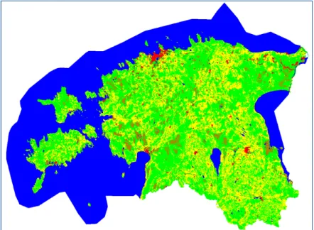
24 Corine2012 model for Estonia. . . 36

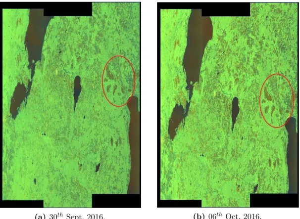
25 30th _{Sept, 2016 from Sentinel-1A and 06}th _{Oct, 2016 from Sentinel-1B. 37} 26 De-bursted interferometric coherence of image pair 30th Sept-06th Oct, 2016 in VV polarization. The coherence scales from 0 to 1. Dark areas are indicating low coherence and bright areas indicating high coherence. 38 27 Multi-looked interferometric coherence of image pair 30th Sept-06th Oct, 2016 in VV polarization. The coherence scales from 0 to 1. Dark areas are indicating low coherence and bright areas indicating high coherence. . . 38

28 Terrain-corrected interferometric coherence of image pair 30th Sept-06th _{Oct, 2016 in VV polarization. The coherence scales from 0 to 1.} Dark areas are indicating low coherence and bright areas indicating high coherence. . . 39

29 Re-projected and re-sampled interferometric coherence of image pair 30th _Sept-06th _{Oct, 2016 in VV polarization. The coherence scales}

from 0 to 1. Dark areas are indicating low coherence and bright areas

indicating high coherence. . . 40

30 Subset of interferometric coherence of image pair 30th _Sept-06th _Oct, 2016 in VV polarization. The coherence scales from 0 to 1. Dark areas are indicating low coherence and bright areas indicating high coherence. 40 31 InSAR processing block diagram. . . 41

32 InSAR processing chain using SNAP. . . 42

33 De-bursted backscatter image of 30th Sept, 2016 in VH polarization. The relative backscattered value ranges from 0 to 1. Dark areas are indicating low backscattering and bright areas are indicating high backscattering. . . 42

34 Multi-looked backscatter image of 30th _{Sept,2016 in VH polarization.} The relative backscattered value ranges from 0 to 1. Dark areas are indicating low backscattering and bright areas are indicating high backscattering. . . 43

35 Terrain flattened and terrain-corrected backscatter image of 30th _Sept, 2016 in VH polarization. The relative backscattered value ranges from 0 to 1. Dark areas are indicating low backscattering and bright areas are indicating high backscattering.. . . 43

36 Speckle filtering of backscatter image of 30th Sept, 2016 in VH polar-ization. The relative backscattered value ranges from 0 to 1. Dark areas are indicating low backscattering and bright areas are indicating high backscattering.. . . 44

37 Re-projected and re-sampled backscatter Image of 30th _{Sept, 2016 in} VH polarization. The relative backscattered value ranges from 0 to 1. Dark areas are indicating low backscattering and bright areas are indicating high backscattering. . . 44

38 Subset of backscatter image of 30th _{Sept, 2016 in VH polarization.} The relative backscattered value ranges from 0 to 1. Dark areas are indicating low backscattering and bright areas are indicating high backscattering. . . 45

39 Backscattering intensity processing block diagram.. . . 45

40 Backscattering intensity processing chain using SNAP. . . 46

41 Re-projection and re-sampling of corine map over Estonia. . . 46

42 RGB image of converged corine map. Classes: Red- Urban; Yellow-Field; Green- Forest; Brown- Peat-land; Blue- Water. . . 47

43 Interferometric coherence image in VH polarization. The coherence scales from 0 to 1. Dark areas are indicating low coherence and bright areas indicating high coherence. . . 49

44 Histogram of interferometric coherence in VH polarization (30th Sept-06th _{Oct, 2016). . . . . 49}

46 Histogram of interferometric coherence in VV polarization (30 Sept-06th _{Oct, 2016). . . . . 50}

47 Backscattering intensity image in VH polarization. The relative backscattered value is converted to decibel (dB). Dark areas are indicating low backscattering and bright areas are indicating high backscattering. . . 51

48 Histogram of backscattering intensity in VH polarization (30th Sept, 2016). . . 52

49 Backscattering intensity image in VV polarization. The relative backscattered value is converted to decibel (dB). Dark areas are indicating low backscattering and bright areas are indicating high backscattering. . . 52

50 Histogram of backscattering intensity in VV polarization (30th Sept, 2016). . . 53

51 Backscattering intensity image in VH polarization. The relative backscattered value is converted to decibel (dB). Dark areas are indicating low backscattering and bright areas are indicating high backscattering. . . 53

52 Histogram of backscattering intensity in VH polarization (06th Oct, 2016). . . 54

53 Backscattering intensity image in VV polarization. The relative backscattered value is converted to decibel (dB). Dark areas are indicating low backscattering and bright areas are indicating high backscattering. . . 54

54 Histogram of backscattering intensity in VH polarization (06th Oct, 2016). . . 55

55 Classification results over Estonia using CohVV + bsVH. Classes: Red- Urban; Yellow- Field; Green- Forest; Brown- Peat-land; Blue-Water. . . 56

56 Classification results over Estonia using CohVH+bsVV. Classes: Red-Urban; Yellow- Field; Green- Forest; Brown- Peat-land; Blue- Water. 57

57 Classification results over Estonia using (VH+VV) coherence. Classes: Red- Urban; Yellow- Field; Green- Forest; Brown- Peat-land; Blue-Water. . . 58

58 Classification results over Estonia using (VH+VV) backscatter. Classes: Red- Urban; Yellow- Field; Green- Forest; Brown- Peat-land; Blue-Water. . . 59

List of Tables

1 Characteristics of Sentinel-1 interferometric wide swath mode. . . 33

2 Sentinel-1 SLC data product parameters. . . 33

3 Sentinel-2A data product parameters. . . 35

4 Geo-coordinates specification for study area. . . 41

5 Conversion of Corine map into 5 major classes.. . . 47

6 Basic parameters calculation for master/slave image. . . 48

7 (Coh-VV + bs-VH) confusion matrix. . . 56

8 (Coh-VH + bs-VV) confusion matrix. . . 57

9 Interferometric coherence (VH + VV) confusion matrix. . . 58

agricultural areas, forests, wetlands and water bodies [1]. On the other hand, land use is a representation of present and future activities by humans on land [2, 3], identified as industrial, commercial, forestry and leisure. Land cover/use information is of great importance for scientific research and applications. Land cover plays a vital role in the geographical analysis ranging from the study of earth sciences to environmental analysis. Land cover maps need to be updated regularly, as they act as a catalyst between socio-economic activities and regional environmental changes. Land cover classification is an important application of remote sensing. Past studies have investigated the efficient usage of remote sensing data for both local and global scale thematic characterization [4]. Moreover, remotely sensed images can be used for consistent and continuous monitoring of Earth’s surface to identify the changes in land cover over large areas [5]. In many studies [6, 7, 8], SAR data has been investigated and proven effective for land cover monitoring.

Technological breakthroughs in remote sensing enable us to monitor dynamics of the Earth surface. Precise and reliable information is required to detect the land change and monitoring of the area of interest. Over the past few years, many optical and Synthetic Aperture Radar (SAR) satellite missions have been launched. During the period 2013-2016, European based Copernicus programme successfully launched Sentinel-1 [9], and Sentinel-2 constellations. Landsat-8 mission was launched as a collaboration between the U.S. Geological Survey (USGS) and the National Aeronautics and Space Administration (NASA) [10] with high spatial resolution (10-30 m). Sentinel missions data are available on Sentinels data hub, under the management of the European Space Agency (ESA) and is free to use for scientific and technological purposes.

Nowadays, optical imagery is often used for land cover classification. The optical sensors can not operate during night and cloud cover restrict its operability in many areas of the Earth. However, SAR sensor is capable of working almost under all weather conditions and can penetrate through cloud cover. Microwave frequency band of SAR system spans over different wavelengths. The penetration of radar wave depends on chosen wavelength. For example, P-Band has 1 m wavelength and its penetration through surface targets is high as compared to other frequency bands. The decrease in wavelength effects radar wave penetration through the target. The Sentinel-1 radar mission is operating at C-band. The penetration capability of C-band is less than P-band. SAR has restrictions regarding the potential of C-band single polarization intensity images [8]. These limitations can be avoided with InSAR technique. Interferometric SAR (InSAR) enhances the potential usage of backscattering intensity by using interferometric coherence as a complementray information [11]. This study mainly focuses on land cover mapping using InSAR technique.

1.1

Remote Sensing

Remote sensing is the science of collecting information by a remote device which is not in direct contact with the object under investigation [12]. In simple words, spaceborne remote sensing can also be defined as observing the planet Earth from space.

Remote sensing satellites acquire Earth surface imagery from orbit. Data acquisi-tion by satellite sensor is done in different wavelength regions of Electromagnetic Spectrum (EMS). The optical remote sensing uses passive instruments which depend on radiated or reflected energy. The EMS for optical remote sensing spans over visible to near infrared (NIR) up to thermal infrared (TIR) region. However, radar is an active imaging sensor and it uses microwave region of EMS. In the EMS, the selected wavelength region plays an important role for a remotely sensed image. Some of the remotely sensed images represent the reflection of solar energy in the visible and the near infrared regions. However, some are the measurements of the energy emitted by the Earth surface itself in the thermal infrared wavelength region. Microwave remote sensing uses active and passive sensors. In active microwave systems, the remote sensing platform itself is the source of the emitted energy [13], whereas passive microwave sensors depends on external energy source such as Sun.

1.2

InSAR Studies on Land Cover

The topic of this thesis is"Land Cover Classification using Sentinel-1 Radar Mission Interferometry". Sentinel-1 constellation has many operational applications and land cover mapping is one of them. Many studies have already been conducted in land cover mapping using SAR based European missions including ERS-1/2, Envisat, and sentinel-1A. With the launch of Sentinel-1B on April 25, 2016, the Sentinel-1 constellation is complete and operating successfully with 24/7 global coverage. Some of the areas in which remote sensing imagery has many applications include land cover mapping, agriculture, environmental monitoring, Earth-resource mapping, water resource management, disaster monitoring and mitigation, soil mapping, forestry, survey and urban planning, military observations and land cover changes [14].

Previously encouraging results have been achieved using European Remote Sensing (ERS) satellite datasets and different classification methods. Dammert et al.

per-formed classification research in two areas of Sweden. Classification accuracy of 65% to 75% was achieved in Gothenburg into five classes, while for Hokmark it was between 60% and 65% [15]. Dammert used unsupervised segmentation method on multiple Tandem pairs for classification. Strozzi et al. conducted research on three different test sites including Bern, Lozère and Tuusula. Strozzi et al. used both supervised and unsupervised classification algorithms on multiple Tandem pairs and achieved 75% classification accuracy into four classes[16]. Forest/nonforest—classification accuracy of 80% to 85% was achieved. Engdahl et al. achieved an overall classification accuracy for Helsinki metropolitan area was of 90% into six classes with a kappa coefficient of 0.86 [17]. Engdahl used the ERS-1/2 tandem InSAR datasets and two-stage hybrid classifier method for land cover classification. Although, they all

1.3

Motivation

The goal for this study is to investigate the usage of interferometric SAR coherence in combination with backscattering intensity using Sentinel-1 image pair with six days temporal baseline. The work presented in this study focuses on the potential of single pair C-band InSAR data for Sentinel-1 mission in land cover monitoring. The main questions to be answered here are:

1. Will it be possible to achieve results for land cover classification with the Sentinel-1A/B interferometric dataset?

2. Can the interferometric coherence be used with intensity parameter to improve land cover classification?

3. How temporal decorrelation affect land cover classification results?

The supervised classification algorithm is used in order to answer the above mentioned questions. The potential of single pair C-band InSAR data of Sentinel-1 is investigated for land cover mapping using Interferometric Wide (IW) swath mode. The IW mode is the main operational mode over land for Sentinel-1 and it contains an abundance of information relating to land cover monitoring.

1.4

Structure of the Report

The thesis is divided into six chapters. Chapter 1 presents the general discussion about the topic, motivation, research problem and thesis goal. In chapter 2, theory and technical parameters of the SAR interferometry is discussed. The chapter 3 presents the material used for this work. Chapter 4 explains the research methodology containing processing chains of interferometric coherence, backscattering and Corine land cover model. In chapter 5, the results are given with the analysis. Chapter 6 gives the conclusion and future recommendations.

2

Theoretical Background

This chapter covers the theoretical background of the thesis. The chapter has three sections. Section 2.1 explains the basic theory in understanding the working principles and properties of Synthetic Aperture Radar (SAR). Section 2.2 gives necessary concepts for better understanding of SAR interferometry (InSAR). Section 2.3 present the methods and techniques used for land cover classification. Mostly, the literature review is based on [12, 13, 20].

2.1

Overview of Radar and SAR

The term Radar stands for Radio Detection and Ranging. A radar is an object detection system that measures the distance (range), angle or velocity to an object. The electromagnetic signals are transmitted to the ground from radar and reflected echo is received from the target. A radar system consists of a transmitter, receiver, transmitting and receiving antennas and processor to process the received echoes shown in Fig.1.

Figure 1: Elements of radar system.

Range or distance to the target can be calculated by measuring the time it takes the electromagnetic signal to propagate to the object and back to the receiver. The electromagnetic signal travels at the speed of light. The signal travels from transmitting antenna to the object and then propagates back to the receiving antenna after reflecting from the object. The electromagnetic signal travels twice the distance between the radar and ground target [13]. Therefore, the range (R) can be calculated as

R= 1

Radar is an active remote sensing instrument. It has its own source of energy. It does not depend on ambient radiation like optical and infrared sensors. Radar can detect and measure the range of relatively small objects at near or far range with precision during day or night. Imaging remote sensing radars, such as SAR, produce high-resolution images of Earth surface. They provide geophysical information by using post-processing techniques on high resolution images. SAR uses backscattered echoes to gather surface information and produce high resolution images [13].

SAR is a side looking microwave imaging system. Remote senisng techniques have been using SAR system for more than 30 years. Being an active system and usage of microwaves enhance its operational capabilities. To acheive the accurate measurements of radiation travel path, interferometric method is useful in SAR systems. The travel path variations in imaging radars can be measured by using satellite position and acquitsition time, which is helpful in generating digital elevation models (DEM) [18].

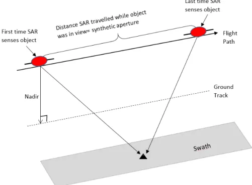
Figure 2: Spaceborne SAR measures distance between spacecraft and the object along the direction of flight.

The principle of SAR instruments is similar to conventional radar. Radar transmit electromagnetic waves and measure the intensity of backscattered echoes by the radar antenna mounted on a moving platform. The time it takes the electromagnetic signal to reach the target and received back at the antenna tells how far is the target from the SAR platform. The SAR measures the distance between the satellite and the ground targets in the direction of flight shown in Fig.2. The radar has a restriction

to the physical length of the antenna mounted on a moving platform. In SAR, the resolution in azimuth is proportional to the size of the antenna. In order to achieve better resolution in azimuth, the physical size of the antenna needs to be increased which is often not practically possible. Moreover, shortening the wavelength will limit its penetration through the cloud cover. To overcome these limitations, SAR uses doppler history of the backscattered echoes. Forward motion of SAR platform generates backscattered echoes which synthesizes a large antenna. Thus, it becomes possible to acquire high resolution image irrespective of small size of physical antenna.

SAR technology has various applications. It provide terrain structural information to geologists for mineral exploration, oil spill boundaries on water to environmentalists, sea state and ice hazard maps to navigators, and targeting information to military operations. SAR applications for civilian usage have not yet been adequately explored. The lower cost electronics are just beginning to make SAR technology economical for smaller scale uses [19].

2.1.1 Principles of Imaging Radar

SAR system is mounted on a moving platform and includes various components: a transmitter, a receiver, an antenna and a recorder. The transmitter generates electromagnetic signal and send the signal to the transmitting antenna. The antenna transmits the signal to ground surface. The receiver collects the backscattered energy as received by the receiving antenna, filters and amplifies for recording. Finally, the recorder then stores the received signal for post processing.

Image acquired by radar is presented in the form of pixels. Each pixel contain digital number which represents the intensity of the backscattered signal. This backscattered signal is received at the receiving antenna. Each transmitted pulse from radar carries energy which can be expressed by radar equation [20] as

Pr =

G2_λ2_P

tσ

(4π)3_R4 , (2)

where Pr is the received power, λ is the wavelength, G is the gain of antenna,Pt is

the transmitted power, σ is the radar cross section and Ris the range from sensor to the target.

Some factors effecting the strength of the backscattered signal are:

• properties of radar system including wavelength, antenna and transmitted power,

• imaging geometry of radar defines the size of the illuminated area. The size depends on a beam-width, incidence angle and range,

• object characteristics in relation to the radar signal, i.e., surface roughness and composition, and terrain topography and orientation.

microwave pulses at regular intervals, called Pulse Repetition Frequency (PRF) [20]. The PRF are bundled together by the antenna to form a beam. This beam travels through the atmosphere and illuminates a target. It is backscattered and travels through the atmosphere again to reach the antenna where the signal intensity is received. Knowing the speed of light and time interval; the signals needs to pass twice the distance between the object and antenna, the distance (range) between the sensor and object can be derived [20].

The signal is received at a receiver and sampling is performed on a signal pulse. These samples are stored in an image line to create an image. A 2D image is created as the pulses are emitted from the sensor that is mounted on a moving platform and each pulse defines one line. The radar sensor, therefore, measures distances and detects backscattered signal intensities.

2.1.1.2 Imaging Radar Frequency Bands

Imaging radar sensors operate with different frequency bands similarly to optical remote sensing. For better identification of the wavelength ranges, a standard has been established that uses letters to distinguish among the various bands. Radar missions uses different wavelengths depending on the application. The European Sentinel-1 mission uses C-band (freq: 5.405 GHz) radar. C-band has many land applications and it is also used for imaging oceans and ice features as well [21]. The different frequency bands in microwave spectrum are shown in Fig.3.

Figure 3: Microwave spectrum commonly used bands and their notation.

2.1.1.3 Microwave Polarizations

The microwave polarization is important in imaging radar systems. The polarization of radar imagery depends on the orientation of transmitted and received Electro-magnetic Wave (EM). EM waves can be horizontal, vertical or cross polarized. Polarization is defined by the orientation of the electric field vector with respect to

horizontal direction. If the electric field vector oscillates parallel to the horizontal direction, the beam is referred to as horizontally polarized, otherwise vertically po-larized shown in Fig.4. Information regarding different applications can be collected using different polarizations and wavelengths.

Figure 4: Vertically polarized electromagnetic wave of wavelength λ has electric field vector E (orange) in vertical direction. The magnetic field B(blue) is perpendicular to E and both are perpendicular to direction of propagationZ.

The backscattered energy can have a different polarization after reflecting from the object. The Sentinel-1 C-band SAR instrument has one switchable transmit chain and two parallel receive chains [22]. These chains operate in single (HH or VV) polarization as well as in dual (HH+HV or VV+VH) polarizations.

• HH: transmitting and receiving signal in horizontal polarization,

• VV: transmitting and receiving signal in vertical polarization,

• HV: transmit in horizontal and receive in vertical polarization, and

• VH: transmit in vertical and receive in horizontal polarization.

2.1.1.4 Incidence Angle

The incidence angle θi is defined as the angle between the incident radar beam and

the direction normal to the Earth surface. The transmitted microwave energy has dependency on angle of incidence of radar pulse. In general, increasing the incidence angle will decrease the intensity of the received backscattering energy from the surface. The angular relationship between the incident radar beam and the surface layer or target is normally described by the angle of incidence [23] shown in Fig.5. Sentinel-1 operates in four acquisition modes [22] and each mode has a different incidence angle range. In this study, we focus on Interferometric wide (IW) swath mode.

Figure 5: SAR incident angle.

2.1.2 Radar Backscattering Coefficient

Radar backscattering coefficient σo gives information about the surface roughness, moisture content in soil and vegetation cover. The coefficient can be described by comparing the backscattered power with the incident power on surface scatterers. The equation used for computing the radar backscattering coefficient of sensor is generally associated to the SAR image brightness as follows

σo= βo

sinθi

, (3)

whereβo is the radar brightness. The radar brightness is the estimated backscattered

power from the ground target. The radar detects the backscattered power and measure in the slant-range geometry. The brightness does not depend on the incidence angle and the local topography [24]. The backscattering coefficient in decibels is given as

σo(dB) = 10log10(σo), (4) where σo is the radar backscattering coefficient in decibels.

2.1.2.1 Parameters Affecting Radar Backscatter

The scattering of microwave radiation depends on geometrical and dielectric properties of natural land surface [25]. The ground scatterers including urban areas, forest and water exhibit different scattering features. The urban areas are very strong backscatters. Forest shows intermediate backscattering, whereas calm water is a low backscatter because of its surface smoothness. The parameters that effect the backscattering coefficient are as follows:

• Frequency: The penetration depth of the radiation for target area and the relative surface roughness are dependent on the frequency of the incident electromagnetic energy.

• Polarization: Imaging radars can have different polarization configurations as discussed in section 2.1.1.3. The selection of polarization affect the penetration depth of radar wave. The information about the orientation and different layers of scattering elements on surface can be obtained from polarization chosen.

• Roughness: Roughness is independent of radar but it is a relative concept which depends on wavelength and incidence angle. According to the Rayleigh criterion, a surface is considered rough if

h > λ

8cos(θi)

, (5)

and surface is considered smooth if

h < λ

8cos(θi)

, (6)

where h is height of surface variation,λ is wavelength andθi is incidence angle.

• Incidence Angle: As discussed earlier, the incidence angle is the angle between the direction normal to the imaged surface and line of sight of incident wave. Backscattering coefficientσo _{varies with the angle of incidence for most natural}

targets.

• Moisture: The dielectric constant measures electrical properties of surface materials. Permittivity and conductivity are important features of dielectric constant. These two features are highly dependent on moisture content of the material under investigation. Moisture effect the dielectric properties of natural surface materials. Radar reflectivity increases with increase in moisture [13, 20].

2.1.3 Radar Image Geometry

The radar sensor mounted on the platform moves along the orbit in the direction of flight. The ground track of the orbit on the Earth’s surface at nadir is shown in Fig.6. The microwave beam illuminates an area, or swath, on the earth’s surface, with an offset from the nadir. The direction along-track is called azimuth and the direction perpendicular (across-track) is called range.

Figure 6: Side-looking viewing geometry of SAR (Image from [26]).

2.1.3.1 Viewing Geometry

In Fig.7, the viewing geometry of imaging radar sensors is shown. The part of the image that is closest to the nadir track is called near range and the portion of the image that is farthest from the nadir is called far range. The angle between the incident radar beam and local vertical is defined as incidence angle. Moving from near range to far range, the incidence angle increases. The difference between the incidence angle of sensor and local incidence depends on terrain slope and Earth curvature. Local incidence angle θi,local [12] is defined as the angle between the

incident radar beam and the local surface normal as shown in Fig.7. The radar sensor measures the distance between antenna and object. This line is called slant range. The true horizontal distance along the ground corresponding to each measure point in slant range is called ground range [12].

2.1.3.2 Spatial Resolution

In imaging radars, spatial resolution is defined in two directions; azimuth and range directions. Resolution in the azimuth direction is called azimuth resolution and resolution in the range direction is called range resolution. The two parameters which define the spatial resolution in azimuth direction and slant range are: pulse length and antenna beam width. In case of Sentinel-1 SAR, the spatial resolution in IW mode is 2.7 x 22 m to 3.5 x 22 m [27].

2.1.3.3 SAR Range Resolution

Two dimensional (2-D) images are produced by SAR. One dimension in the image is called range (or cross track). Range resolution is determined by the width of the transmitted pulse. The narrow pulses produce fine range resolution. SAR range resolution can be categorized into slant range and ground range. In slant range, two ground objects are separated by a distance and received signal contains two different echoes. The distance between the ground objects define the spatial resolution in the slant range. Range has no effect on the resolution of slant range. However, incidence angle effects the resolution in ground geometry. Slant range resolution δr is constant along the range and is defined as

δr= cτ

2 . (7)

Ground range resolutionRr is not constant across the range and is given as Rr =

cτ

2sinθ, (8)

where c is the speed of light in vacuum, θ is look angle and τ is pulse length in [20].

2.1.3.4 SAR Azimuth Resolution

The second dimension in the image is perpendicular to range and is called azimuth (or along track). The spatial resolution in azimuth direction depends on the beam width and the range. The beam width of radar depends on wavelength and length of antenna. It is proportional to the wavelength and inversely proportional to the antenna aperture. This shows that large antenna will produce narrow beam and high resolution will be achieved in azimuth direction. SAR produces relatively fine azimuth resolution. This ability makes it different from other radars. Azimuth resolution is defined by the beam sharpness. The antenna length effects the sharpness of beam. If the antenna is large, it will focuses the transmitted and received energy into a sharp beam. Therefore, fine azimuth resolution will be achieved with sharp beam. The physical length of the radarRa is proportional to azimuth resolution [20]

and is expressed as

Ra= L

2.1.4 SAR Image Types

A SAR image measures the radar backscattering contributions from the Earth’s surface. This section discusses the differentiation between complex and detected SAR images as well as the concept of different SAR looks.

2.1.4.1 Complex Images

A complex SAR image Z can be expressed mathematically in its amplitude and phase form as

Z(r, a) =A(r, a)eiφ(r,a), (10)

where r and a are image coordinates in range and azimuth, A is amplitude of the image and φ is phase of the image.

Complex SAR images are usually presented in slant range geometry and they have a single look. These kinds of complex images are called Single Look Complex (SLC) images. SLC image retain the amplitude and phase of the original SAR data

[11].

2.1.4.2 Detected Images

As mentioned above, the SAR image contains both the amplitude and phase. The phase information from the SAR images is removed prior to be used for visualisation. Practically, this step is a part of processing chain and is called detection. The strength of the radar signal in each pixel is determined by the detection. Therefore, the resulting images are called the detected images. A square law detection is one of the detection processes. In square law detection, an intensity imageI =A2 _{is formed} by multiplying the complex SAR imageZ with its complex conjugate Z∗ [11].

2.1.4.3 Single-look Image

SLC products are focused SAR images. They use orbit and attitude information from the satellite for geo-referencing [28], and are presented in slant-range geometry. The spatial resolution in SLC images is high. In single look images, the radar reflectivity and radiometric resolution becomes poor due to the speckle effect [11].

2.1.4.4 Multi-looked Image

Multi-looking is a process in which radiometric resolution of SAR data is improved at the expense of spatial resolution. In multi-looking operation, the synthetic aperture is divided into N parts and produce N lower resolution looks. These N looks are produced by single SAR data and then they are averaged together incoherently.

Another approach to multi-looking is to take an incoherent spatial average of a single look SAR image. Radiometric resolution is improved with both of these approaches as they are statistically and produce an N-look SAR image [11].

2.1.5 Distortions in Radar Images

The side-looking viewing geometry causes geometric and radiometric distortions in SAR imagery. Radar images experience variations in scale i.e., slant range to ground range conversion, foreshortening, layover and shadows [12].

2.1.5.1 Slant-Range Scale Distortions

Radar detect and measure ranges to ground objects in slant range. Therefore, the image has different scales moving from near to far range. This means that objects in near range are compressed with respect to objects at far range [12]. For proper interpretation, the image has to be corrected and transformed into ground range geometry. In Fig.8. the targets A1 and B1 are of the same size on the ground but their apparent dimensions appear different in slant range (A2 and B2). This causes targets to appear compressed in the near range as compared to the far range.

Figure 8: Slant-range scale distortion in SAR.

2.1.5.2 Terrain Induced Distortions

Terrain induced distortions are caused by relief displacement and it also effect radar imagery. Relief displacement is one dimensional and occurs in direction perpendicular to flight path. However, the displacement is reversed with targets being displaced towards the sensor. There are three effects that are typical for radar including foreshortening, layover and shadow shown in Fig.9.

Figure 9: Geometric distortions in SAR images.

Foreshortening: Radar measures distance in slant range rather than true hori-zontal along the ground. The slope area is compressed in the image. The slope forms an angle in relation to the angle of the incident radar beam. The slope can be made shortened more or less on the basis of this angle. The distortion is at its maximum if the radar beam is almost perpendicular to the slope [12] as shown in featureD in Fig.9. Foreshortened areas appear bright in the radar image.

Layover:Layover occurs when the radar beam reaches the top of the slope earlier than the bottom [12] as shown in features A and B in Fig.9. At near range, the layover displacement is greater for smaller look angle. Layover areas also appear bright in the image and it can be considered as extreme case of foreshortening.

Shadow: Radar beam cannot illuminate the area of slope which is facing away from the sensor. Therefore, there is weak energy or no energy at all that can be backscattered to the sensor and those regions remain dark in the image. In Fig.9, the right side of feature A will be slightly illuminated as the slope is less steep than the look direction. The features C and D have slopes more steeper than look direction so the shadow extends beyond the slope area as shown in Fig.9. There will be no illumination when the slope facing away from satellite is parallel to the look direction as shown in feature B [12].

2.1.6 Radiometric Distortions

The above mentioned geometric distortions also have an influence on the received energy. Since the backscattered energy is collected in slant range, the received energy coming from a slope facing the sensor is stored in a reduced area in the image. This means it is compressed into fewer image pixels than should be the case if obtained in ground range geometry. This results in high digital numbers because the energy collected from different objects is combined. unfortunately this effect cannot be corrected. This is why especially layover and shadow areas in radar imagery cannot

be used for interpretation. However, they are useful in the sense that they contribute to a three dimensional look of the image and therefore help the understanding of the terrain structure and topography.

A typical property of the radar image is the so called speckle. It appears as grainy in the image shown in Fig.10. Speckle is caused by the interaction of the different microwaves backscattered from the object area. The wave interactions are called interference. Interference causes the return signals to be extinguished or amplified resulting in dark and bright pixels in the image even when the sensor observes a homogeneous area. Image interpretation is difficult as speckling degrades the quality of the radar imagery.

Figure 10:Radar speckle filtering (Image from [29]).

Multi-looking or spatial filtering can be used to reduce the speckle effect. In the case of multi-look processing, the radar beam is divided into several narrower beams. Each beam provides a look at the object. Using the average of these multiple looks, the final image is obtained. Multi-look processing reduces the spatial resolution [30]. Another way to reduce speckle is to apply spatial filters on the images. Speckle filters are designed to adapt to local image variations in order to smooth the values to reduce speckle. Speckle filtering enhance lines and edges to maintain the sharpness of the imagery.

2.1.7 SAR Processing

SAR processing is needed to reconstruct the imaged scene from a number of reflected pulses from each target on the surface of Earth. The reflected pulses are received by the antenna and registered in memory. The signal energy reflected from a point target is spread in two directions; range and azimuth. The Signal is spread in range by the duration of the transmitted pulse. In azimuth, the signal is spread by the duration it is illuminated by the antenna beam. SAR processing is carried out in two

commonly used algorithm for processing SAR data.

2.1.7.1 Range Doppler Algorithm (RDA)

The range to the target changes as the point target passes through the azimuth antenna beam. The change in range causes variation in phase of the received signal as a function of azimuth. This phase variation over the synthetic aperture corresponds to the Doppler bandwidth of the azimuth signal. It allows the signal to be compressed in the azimuth direction. The variation in range to point target can cause variation in range delay which is larger than the range sample spacing. This is called range migration. This range migration of the signal energy must be corrected before azimuth compression can occur. The Range-Doppler algorithm is used to perform this correction [31].

There are various steps in RDA including range compression, azimuth Fast Fourier Transform (FFT), Range Cell Migration Correction (RCMC) and azimuth compression as shown in Fig.11.

Figure 11: Steps for range doppler algorithm.

• Range Compression: Radar transmits linear FM pulses during SAR data acquisition. Linear FM pulse uses matched filter to give a narrow pulse. All the energy in the pulse is collected to the peak value. Applying match filtering

to received echo with its corresponding resolution and signal-to-noise ratio is called range resolution. Range compression is performed efficiently using FFT to each range line.Range compression data is obtained by applying an inverse FFT (IFFT) to each line. Range compressed data is then multiplied by a vector that correct the effects caused by the elevation beam pattern and range spreading loss on the amplitude [32].

• Azimuth FFT: Data is transformed into range doppler domain by using FFT in azimuth direction [32].

• Range Cell Migration Correction (RCMC): RCMC is applied to correct the change in range delay to a point target. This range depends on the zero-Doppler range and on the angle from the satellite to the target. Ground targets with same zero-Doppler range have same range variation from the radar. The shape of the signal trajectories are same but they have azimuth displacement. Targets having the same zero-Doppler range can be expressed as a function of Doppler frequency. Due to this, RCMC performs efficiently in the range Doppler domain. The shift in range is needed to align the signal trajectory in a single range bin. It is determined independently for each azimuth frequency bin. The shift is then implemented by an interpolation in the range direction [32].

• Azimuth Compression: FFT is used to perform match filtering of azimuth signal. The match filtering of the azimuth signal is called azimuth compression. At this point, azimuth FFT has already been performed. The frequency response of the azimuth compression filter is precomputed using the orbital geometry. The azimuth filter also depends on range. Thus the data is divided into range invariance regions. The same basic matched filter is used over a range interval called the FM rate invariance region. The size of this invariance region must not be large enough to cause severe broadening in the compressed image. Focused SAR image is resulted after applying IFFT to each azimuth line [32].

2.2

InSAR Fundamentals

This section gives history and introduction to InSAR. Interferometric phase and coherence has been discussed to give the insight of InSAR basic theory and concepts for better understanding.

2.2.1 Introduction

SAR interferometry was first used for analyzing the surface of Venus and Moon from Earth by using the InSAR configurations with antennas [33]. The concept of topographic mapping by using synthetic aperture radar was first introduced by [34] and the first practical observations using airborne radar was presented in [35]. Goldstein et al. applied InSAR technique for the first time in space [36]. SEASAT-A

improved the feasibility of InSAR in space [37]. They provide interferometric data with 24 hour temporal baseline. The Sentinel-1 constellation has also improved the potential of SAR interferometry in various applications including land cover mapping.

Over the past many years, digital elevatin models (DEM) of the Earth surface have been produced using Interferometric SAR technique [38]. Interferometry method uses two radar images to achieve coherence and phase difference between the images. The distance between the satellite and the ground object determines the phase of the SAR image. After coregistration, the phase of two images are combined to generate an interferogram. The phase of generated interferogram is high correlated to terrain topograpghy. Mostly DEMs derived from interferometry method use two antennas that are mounted on an aircraft or spaceborne platform, acquiring data simultaneously [38]. However, single sensor can be used for producing DEMs if same flight track is followed repeatedly. Temporal baselines effect interferometric coherence. Long temporal baseline decreases the coherence. The surface scatter changes its position and structure with time between radar acquisitions. This intorduces intrinsic changes in surface reflectivity causing phase noise to increase[39] and elevation measurement accuracy to decrase [40].

Remote sensing and geodesy uses interferometric SAR technique. This technique uses atleast two SAR images. Maps of surface deformation are generated by us-ing the phase difference of the echoes received at the sensor after reflectus-ing from ground surface. With InSAR, even centimetric scale changes in deformation can be detected and measured. It provide services for monitoring of natural hazards, for example, earthquakes, volcanoes and landslides. It also has applications in structural engineering, in particular monitoring of subsidence and structural stability.

2.2.1.1 Types of SAR Interferometry

There are two types of SAR interferometry; cross track interferometry (XTI) and along track interferometry (ATI). In corss track interferometry, two radar antennas are arranged across the track of the platform. XTI can be subdivided into single pass and repeat pass interferometry. Single pass XTI has two separate antennas mounted on the same platform. The SRTM mission uses single pass cross track interferometry. Repeat pass XTI uses single sensor mounted on the platform. It uses two separate passes of a single antenna as for Sentinel-1 mission. The repeat pass XTI always operates in the ping pong mode. However, the single pass arrangement can operate in either ping pong or standard mode depending on the design of the system [41].

Another type is along track interferometry. In ATI, radar antennas are arranged parallel to velocity vector of the platform. Similarly ATI, can be subdivided into single pass and repeat pass interferometry. Single pass ATI have two antennas arranged fore and aft on the fuselage of aircraft systems as shown in Fig.12. Their operating mode is either standard or ping pong. Repeat pass ATI has single radar antenna, following the same orbital track repeatedly. The along track interferometry

is important for detecting changes between SAR acquisitions. However, it is not sensitive to terrain variations since slant ranges are the same. Practically, in along track interferometry, the platforms do not follow the same path. Moreover, there is some along track separation as well as cross track separation which leads to detect terrain changes and topographic details [41].

Figure 12: Types of SAR interferometry (Image from [42]).

Sentinel-1 mission orbits the Earth in the along track repeat pass configuration. The time interval between SAR acquisitions is 12 days with single satellite and 6 days with two satellites. The distance between the two satellites in the plane perpendicular to the orbit is called the interferometer baseline and its projection perpendicular to the slant range is the perpendicular baseline.

2.2.1.2 InSAR Baselines

SAR satellites are usually launched in Leo Earth Orbit (LEO) around the Earth at an altitude of about 500-800 km and revisit the same location on Earth after a specified time. The time period between the two successive SAR acquisitions is called

temporal baseline. The revisit time of satellites can be several days and extend to

a month depending on the satellite orbit. Past studies have shown that the SAR observations with the shortest temporal baselines produce high coherence results. The temporal baseline for Sentinel-1 radar mission is 12 days with one satellite and reduces to six days with full constellation. However, the satellite location will be a bit changed while acquiring the next observation due to its restrictions in orbit control. In Fig.13, theperpendicular baselinedefines the distance between two acquisition

Figure 13: Perpendicular baseline for InSAR.

For InSAR, it is advisable to use suitable temporal and perpendicular baselines in combination with the area of interest and the availability of SAR data. In InSAR method, the phase from two or more images are compared in each pixel and phase is supposed to be consistent so that it can be used for comparison. If the images acquired have short temporal baseline, the scattering elements on the Earth surface will maintain its structure and position and high coherent values will be achieved otherwise there are chances that objects will change in case of longer temporal baseline. Changes affect coherence and can lead to decorrelation between the two pixels. ERS 1/2 mission has 24 hours temporal baseline between the acquisitions and therefore provides high coherence results. This causes a loss of coherence and eventually leads to complete decorrelation between the two pixels. Perpendicular baseline also has an effect on coherence. Larger baselines causes loss in coherence as target looks different with viewing angle.

2.2.2 Interferometric Phase for Terrain Altitude Measurement

In repeat pass interferometry, SAR systems observe the point scatterers on the surface of Earth from two slightly different look angles. The two observations in ground resolution cell cannot be taken from exactly the same location due to some orbit control limitations. The interferometric phase of the SAR image pixels is the difference in the travel paths of the two SAR sensors to the considered ground resolution cell. This difference cancels out any phase contributed to the interferometric phase by the point scatterers. In passing from identified reference cell to another, introduces variation in the travel path difference ∆r [43]. The travel path variation depends on geometric parameters and can be expressed as

∆r =−2Bnqs

where Bn is the perpendicular baseline, R is the range between sensor and target,

andqs is the displacement between the resolution cells along the perpendicular to

the slant range. The ∆r expression is an approximation for small baselines and small distance resolution cells. The interferometric phase variation ∆φ [43] is proportional to ∆r divided by the transmitted wavelength λ and can be expressed as

∆φ = 2π∆r λ = 4π λ Bnqs R . (12) 2.2.2.1 Interferogram Flattening

The interferogram flattening is a part of InSAR processing and provides accurate topographic information. The purpose is to remove the phase contribution from flat earth as it has nothing to do with surface deformation or topographic elevation [44]. The interferometric phase variation ∆φ can be divided into two terms. In equation 13, the first term represents a phase variation proportional to the altitude difference between the point targets. The second term represents a phase variation proportional to the slant range displacement of the point targets [43].

∆φ=−4π λ Bnq Rsinθ − 4π λ Bns Rtanθ, (13)

where θ is the radiation incidence angle with respect to the reference, q is the difference in altitude between targets, and s is the displacement of the targets in slant-range. The calculation of perpendicular baseline requires precise orbital data. For interferogram flattening, the second phase term is calculated and subtracted from the interferometric phase. As a result, it generates a phase map proportional to the relative terrain altitude [43].

2.2.2.2 Height of Ambiguity

The height of ambiguity ha is the amount of height change that generates 2π change

in interferometric phase. Theha leads to an interferometric phase change of 2π after

interferogram flattening. The height of ambiguity is inversely proportional to the perpendicular baseline [43] and is expressed as

ha =

λRsinθ

2Bn

. (14)

Practically, the phase noise is equivalent to smaller altitude noise so longer baselines gives accurate altitude measurement. Moreover, the higher the baseline, the smaller the topographic height needed to produce a fringe of phase change or, the longer the baseline is the stronger the topographic imprint. The perpendicular baseline needs to be in the limit, otherwise interferometric signals decorrelate and no fringe will be generated. To sum up, signal to noise power ratio is maximised by optimum perpendicular baseline [43].

etc [45]. System noise and terrain change cannot be avoided. On the other hand, images misregistration and geometric decorrelation can be taken care of. System noise is small comparatively with sensed signals, and the processing noise can be controlled if the processor is designed to preserve the phase [46]. It is observed that fringe quality is mainly degraded with scattering change in time and volumetric effects. The complex interferometric coherenceγ is the complex correlation coefficient between two SAR images [11] and is expressed as

γ = E[ ¯Z1Z¯2 ? ] q E[ ¯Z1]2E[ ¯Z2]2 , (15)

whereE[] denotes the expected value and * denotes the complex conjugate. The phase of the complex coherence gives the expected value of the interferometric phase of the observed pixel. The interferometric phase is the phase of the complex correlation coefficient [11] and is expressed as

φ =arg{γ}=arg{E[ ¯Z1Z¯2

?

]}, (16)

and its two dimensional map is called the interferogram.

The interferometric coherence carries key information about the target depending on the radar wavelength chosen. The coherence varies from 0 to 1 due to scaling by the denominator. Incoherence is indicated with 0 and perfect coherence is indicated with 1. The presence of noise in interferometric phase causes decrease in coherence. High coherence values are achieved when both images experience same or nearly the same interaction with ground scatterers. This way both images will have a similar speckle pattern [47]. The signal to noise ratio (SNR) of the interferogram can be expressed in relation to coherence [11] as

SN R= |¯γ|

1− |γ¯|. (17)

2.3

Land Cover Classification

Land cover is a physical representation of various processes taking place on the Earth’s surface. It provides information about the various contents by which the land is occupied including natural sources such as forest and woodlands. It also indicate the way in which the land is being used. Classification is a way of classifying land cover contents into different classes using well defined classifiers. It is defined as the ordering or arrangement of objects into groups or sets on the basis of their relationships [48]. A classification is a system of recognizing and assigning class names to different objects and using a criteria to distinguish relationship between these classes. Classification needs an objective criteria which needs to define class boundary depending on precision, clarity and quantity. A classification procedure

should be independent of any scale and source. Classes can be applied to any level of details and sources of collecting information must not be restricted means it can be a satellite imagery, aerial images, on field data or using fusion of sources.

The major goal of satellite remote sensing is acquiring land images, interpretation and classification of features. Besides photo interpretation, quantitative analysis is a form of classification which labels every pixel in an image to particular spectral class. The purpose of image classification is assigning classes to all image pixels. Every pixel has a digital number (DN) which defines the spectral reflectance and is a basis of classification. Classification can be divided in to two basic methods: supervised classification and unsupervised classification. The supervised classification is the essential tool used for extracting quantitative information from remotely sensed image data [49]. Using supervised method, training samples are collected from the available image pixels for each class of interest. This operation is called training. Classifiers are trained using the selected training samples to assign labels to every pixel in the image. Another method of classification is unsupervised classification. Unsupervised classification does not require any prior knowledge of the classes to label the pixels. It uses clustering algorithms to assign classes to image pixels [49].

2.3.1 Classification Techniques

Many classification methods have been developed and used for generating land cover maps [50]. Supervised and unsupervised classification are the two basic classification techniques. Here, we will give the overview of both classification methods.

2.3.1.1 Unsupervised Classification

The unsupervised classification does not use prior knowledge of training samples to assign classes to the image data. In this method, same values are assigned to the pixels belonging to same class. Clustering algorithm uses natural groupings or clusters. The number of clusters and band selection is done by the user. Image classification tools generate groups or clusters using this information. Different algorithms are used for image clustering, for example, ISODATA and K-means. Reference data is used to compare with the results to decide the classes of clusters or groups.

Image pixels are grouped together based on their reflectance or emittance proper-ties. These groupings are called clusters. In unsupervised classification, the operator manually distinguishes each cluster with respect to land cover class. There are high chances that single land cover class is represented by multiple clusters. It is then advisable to merge the clusters into one land cover type. The unsupervised image classification technique is commonly used when no sample sites exist. The unsupervised classification has three main steps: generation of clusters, assigning classes and validation of results [12]. In Fig.14, the flow diagram of unsupervised classification is shown.

Figure 14: Unsupervised classification flow diagram.

2.3.1.2 Supervised Classification

The supervised classification uses prior knowledge of training samples to train the classifiers and to assign classes to the image data. This procedure of pixel categorization is called the supervised. Supervised classification uses reference data for extracting spectral features of some areas from knonw land cover types [51]. The extracted areas are called "training areas". Training samples generate spectral signatures. These signatures are then used to train the classifier for classifying the spectral data into a thematic map [52]. Image pixels are then classified depending on the similarity of spectral features with the spectral features of the training areas. The analyst identifies the training area and develops a numerical description of the spectral attributes of the class or land cover type. During the training stage, size, shape, location and orientation of pixels for each class is determined. The spectral signatures are compared with the unknown pixels in the image. The unknown pixels will be labelled according to their digital resemblance with the nearby class. Similarly, supervised classification has three main steps: selection of training areas, pixel labelling and validation of results [12]. The flow diagram of supervised classification is shown in Fig.15.

Figure 15: Supervised classification flow diagram.

2.3.2 Types of Classifier

In this study, supervised classification technique has been used for land cover classifi-cation. Supervised classification has different classifiers to be used, depending on their purpose and performance. Euclidean distance and k-nearest neighbour (kNN) classifiers are utilised for the study purpose and will be discussed further.

2.3.2.1 Euclidean Distance

Euclidean distance has nothing to do with machine learning specifically. It is only one of the many available options to measure the distance between two data objects. However, many classification algorithms (for e.g. K-Nearest Neighbour, Minimum Distance Classifier etc) use it to either train the classifier or decide the class membership of a test observation and clustering algorithms (e.g. k-means) use it to assign membership to data objects among different clusters.

Euclidean distance D measures the distance between two points in any number of dimensions. It is expressed mathematically as the square root of the sum of the squares of the differences between the respective coordinates in each of the dimensions [53] D(m, p) = v u u t n X i=1 (mi−pi)2, (18)

where m is the unknown feature vector,p is the training sample and n shows the number of dimensions of feature vectors.