Semantic Document Clustering Using Information
from WordNet and DBPedia
Lubomir Stanchev
Computer Science Department California Polytechnic State UniversitySan Luis Obispo, CA, USA [email protected]
Abstract—Semantic document clustering is a type of unsu-pervised learning in which documents are grouped together based on their meaning. Unlike traditional approaches that cluster documents based on common keywords, this technique can group documents that share no words in common as long as they are on the same subject. We compute the similarity between two documents as a function of the semantic similarity between the words and phrases in the documents. We model information from WordNet and DBPedia as a probabilistic graph that can be used to compute the similarity between two terms. We experimentally validate our algorithm on the Reuters-21578 benchmark, which contains 11, 362 newswire stories that are grouped in 82 categories using human judgment. We apply the k-means clustering algorithm to group the documents using a similarity metric that is based on keyword matching and one that uses the probabilistic graph. We show that the second approach produces higher precision and recall, which corresponds to better alignment with the classification that was done by human experts.
I. INTRODUCTION
Consider an RSS feed of news stories. Organizing them in categories will make search easier. For example, a smart classifier will put a story about “Tardar Sauce” (better known as Grumpy Cat) and a story about “Henri, le Chat Noir” (Henry, the black cat) in the same category because both stories are about famous cats from the Internet. Our approach uses information from WordNet [25] and DBPedia [20] to construct a probabilistic graph that can be used to compute the semantic similarity between the two documents.
The problem of semantic document clustering is interesting because it can improve the quality of the clustering results as compared to keyword matching algorithms. For example, the later algorithms will likely put documents that use different terminology to describe the same concept in separate cate-gories. Consider a document that contains the term “ascorbic acid” multiple times and a document that contains the term “vitamin C” multiple times. The documents are semantically similar because “ascorbic acid” and “vitamin C” refer to the same organic compound and therefore a clustering algorithm should take this fact into account. However, this will only happen when the close relationship between the two terms is stored in the system and applied during document clustering. The need for a semantic document clustering system becomes even more apparent when the number of documents is small or when they are very short. In this case, it is likely that the documents will not share many words and a keyword matching
strategy will struggle to find evidence for grouping any two documents together.
The problem of semantic document clustering is difficult because it involves some understanding of the English lan-guage and our world. For example, our system can use infor-mation from DBPedia to determine that “Henri, le Chat Noir” and “Tardar Sauce” are both famous Internet cats. Although significant effort has been put forward in automated natural language processing [9], [10], [23], current approaches fall short of understanding the precise meaning of human text. In our approach, we make limited use of natural language processing techniques (for example, we use the Standford CoreNLP tool [22]) and we rely on high-quality information about the words in English language (WordNet) and our world (DBPedia) to process the input documents.
A traditional approach uses k-means clustering [21] to clus-ter documents. The algorithm is based on a vector representa-tion of the documents (based on term frequencies) and a dis-tance metric (e.g., the cosine similarity between two document vectors). Unfortunately, this approach will incorrectly compute the similarity distance between two documents that describe the same concept using different words. It will only consider the common words and their frequencies and it will ignore the meaning of the words. In [41], we explore how information from WordNet can be used to create a probabilistic graph that is used to cluster the documents. However, this approach does not take into account information from DBPedia and will not be able to determine that “Tardar Sauce” and “Henri, le Chat Noir” are both famous Internet cats.
In this paper, we extend the approach from [41] in two ways. First, we apply the Standford CoreNLP tool to lemmatize the words in the documents and assign them to the correct part of speech (i.e., noun, verb, adjective, or adverb). Second, we add information from DBPedia to the probabilistic graph. DBPedia contains knowledge from Wikipedia. This includes the title of each Wikipedia page, the short abstract for the page, the length of the Wikipedia page, the category of each Wikipedia page (e.g., “Anarchism” belongs to the category “Political Cultures”), information that an object belongs to a class (e.g., “Azerbaijan” is a type of a country), RDF triplets between objects (e.g., “Algeria” has official language that is “Arabic”), and about disambiguation (e.g., “Alien” can refer to “Alien(law)”, that is, the legal meaning of the word.) All this
information allows us to extend the probabilistic graph and find new evidence about the semantic similarities between the phrases in the documents that are to be clustered.
In what follows, in Section II we present an overview of related research. Our main contribution is in Section III, where we present a modified algorithm for creating the probabilistic graph that stores the part of speech for each word. The algorithm is then extended with information from DBPedia. Section IV describes our algorithms for measuring the semantic similarity between documents and clustering the documents. Our other contribution is in Section V, where we describe our implementation of the algorithm using a distributed Hadoop environment and validate our approach by showing how it can produce data of better quality than the algorithm that is based on simple keywords matching and our previous algorithm that relies exclusively on data from WordNet. Lastly, Section VI summarizes the paper and outlines areas for future research.
II. RELATED RESEARCH
The probabilistic graph that is presented in this paper is based on the research from [37], which shows how to measure the semantic similarity between words based on information from WordNet. Later on, in [38] we explain how the graph can be extended with information from Wikipedia. After that, in [40] we show how the Markov Logic Network model [29] can use the probabilistic graph to compute the probability that a word is relevant to a user given that a different word from the user’s input query is relevant. Lastly, in [36] we show how a random walk in a bounded box in the graph can be used to make the computation of the semantic similarity between two words more precise and more efficient. In this paper, we extend this existing research in two ways: (1) we store the part of speech together with each word in the graph and (2) we incorporate knowledge from DBPedia in the probabilistic graph.
Note that a plethora of research papers have been published on the subject of using supervised learning models with train-ing sets for document classification [5], [42]. Our approach differs because it is unsupervised, it does not use a training set, and it can cluster documents in any number of classes rather than just classify the documents in preexisting topics.
One alternative to supervised learning is using a knowledge-base that contains information about the relationship between the words and phrases that can be found in the documents to be clustered. For example, in 1986, W. B. Croft proposed the use of a thesaurus that contains semantic information, such as what words are synonyms [7]. Sequentially, there have been multiple papers on the use of a thesaurus to represent the semantic relationship between words and phrases [14], [30]. This approach, although very progressive for the times, differs from our approach because we consider indirect relationships between words (i.e., relationships along paths of several words). We also do not apply document expansion (e.g., adding the synonyms of the words in a document to the document) when comparing two documents. Instead, we use
the probabilistic graph to compute the distance between two documents. Some limited user interaction is possible when classifying documents – see for example the research on folksonomies [11]. Our system currently does not allow for user interaction when creating the document clusters.
In later years, the research of Croft was extended by creating a graph in the form of a semantic network [4], [28], [31] and graphs that contain the semantic relationships between words [2], [1], [6]. Later on, Simone Ponzetto and Michael Strube showed how to create a graph that only represents inheritance of words in WordNet [18], [32], while Glen Jeh and Jennifer Widom showed how to approximate the similarity between phrases based on information about the structure of the graph in which they appear [15]. All these approaches differ from our approach because they do not consider the strength of the relationship between the nodes in the graph. In other words, weights are not assigned to the edges of the graph.
Natural language techniques can be used to analyze the text in a document [13], [26], [35]. For example, a natural language analyzer may determine that a document talks about animals and words or concepts that can represent an animal can be identified in other documents. As a result, documents that are identified to refer to the same or similar concepts can be classified together. One problem with this approach is that it is computationally expensive. A second problem is that it is not a probabilistic model and therefore it is difficult to be applied towards generating a document similarity metric.
Note our limited use of ontologies to cluster the documents. Unlike existing approaches that annotate each document with a description in a formal language [17], [27], [12], we use ontological information from DBPedia to calculate the weights of the edges in the probabilistic graph. The problem with the traditional approach is that: (1) manual annotation is time consuming and automatic annotation is not very reliable and (2) a query language, such as SPARQL [33], can tell us which documents are similar, but it will not give us a similarity metric.
Since the early 1990s, research on LSA (stands for latent semantic analysis [8]) has been carried out. The approach has the advantage of not relying on external information. Instead, it considers the adjacency of words in text documents as proof of their semantic similarity. For example, LSA can be used to detect words that are synonyms [19]. This differs from our approach because we do not consider the location of the words in the documents for the most part. The only exceptions are when we extract the part of the speech for each word and when we compute the conditional probability between a sense and the words in the sense and give higher weight to do first words because they are more relevant.
Lastly, not that our approach is different from that of Word2Vec ([24]). Word2Vec explores existing documents to find which words go together. Instead, we use high quality knowledge from WordNet and DBPedia to find the degree of semantic similarity between phrases.
[chair,wf noun]⇒[aseatforoneperson,s noun],35/39
[aseatforoneperson,s noun]⇒[chair,wf noun],1
[aseatforoneperson,s noun]⇒[seat,wf noun],0.6 [aseatforoneperson,s noun]⇒[person,wf noun],0.4
III. BUILDING THE PROBABILISTIC GRAPH In this section, we extend on previous approaches to build-ing the probabilistic graph [38], [41] by considerbuild-ing the part of speech for each word and using information from DBPedia. A. Modeling WordNet
WordNet gives us information about the words in the English language. We use WordNet 3.0, which contains about
150,000different terms. Both words and phrases can be found in WordNet. For example, “sports utility vehicle” is a term from WordNet. WordNet uses the terminology word form to refer to both words and phrases. Note that the meaning of a word form is not precise. For example, the word “spring” can mean the season after winter, a metal elastic device, or natural flow of ground water, among other meanings. This is the reason why WordNet uses the concept of a sense. For example, earlier in this paragraph we cited three different senses of the word “spring”. Every word form has one or more senses and every sense is represented by one or more word forms. A human can usually determine which of the many senses a word form represents by the context in which the word form appears. Each word form is classified in one of four categories: noun, verb, adjective, or adverb.
WordNet contains a plethora of information about word forms and senses. For example, it contains the definition and example use of each sense. Consider the word “chair”. One of its senses has the definition: “a seat for one person, with a support for the back” and the example use: “he put his coat over the back of the chair and sat down”. Two other senses of the word have the definitions: “the position of a professor” and “the officer who presides at the meetings of an organization”. We process these textual descriptions to extract evidence about the strength of the relationship between a word form and the word forms that appear in the definition and example use of the word’s senses. Note that WordNet also provides information about the frequency of use of each sense. This represents the popularity of the sense in the English language relative to the popularity of the other senses of the word form. For example, in WordNet the first sense of the word “chair” (a seat for one person, with a support for the back) is given a frequency of 35, the second sense (the position of a professor) is given frequency of just two, while the third sense (the officer who presides at the meetings of an organization) is given a frequency of one.
WordNet also contains information about the relationship between senses. The senses in WordNet are divided into four categories: nouns, verbs, adjectives, and adverbs. For example, WordNet stores information about the hypernym and hyponym relationships between nouns. The hypernym relationship corre-sponds to the “kind-of” relationship. For example, “canine” in a hypernym of “dog”. The hyponym relationship is the reverse. For example, “dog” is a hyponym of “canine”. WordNet also provides information about the meronym and holonym relationship between noun senses. The meronym relationship corresponds to the “part-of” relationship. The holonym re-lationship is the reverse of the meronym rere-lationship. For
example, “building” is a holonym of “window”. For verbs, WordNet defines the hypernym and troponym relationships. X is a hypernym of Y if performing X is one way of performing Y. For example, “to perceive” is a hypernym of “to listen”. The verb Y is a troponym of the verb X if the activity Y is doing X in some manner. For example, “to lisp” is a troponym of “to talk”. Lastly, WordNet defines the related to and similar to relationship between adjective senses, which are self explanatory.
We create a node in the probabilistic graph for each word form and part of speech pair. For example, we create a node for [spring, wf noun] and a node for [spring, wf verb], where wf stands for word form. The first node represents the word form noun “spring”, while the second node represents the word form verb “spring”. In this paper, we consider the two word forms to be distinct entities and we do not explicitly create an edge between them just because they share the same syntax. We also create a node for each sense. For example, we create a node with label [natural flow of ground water, s noun], where s stands for sense. Instead of revisiting our previous algorithm from [40], we summarize how the probabilities are computed in Table I, where these probabilities are used to create the weighted edges between the nodes. The different constants that appear in the formulas were determined using experimental evaluation [39]. The formulas are slightly modified and we do some extra processing to process the part of speech for each word form node and for each sense node. Next, we show few examples that demonstrate the algorithm for creating the probabilities.
Consider the noun chair and its most popular meanings: “a seat for one person”. In total, the noun has four meaning, where WordNet defines their frequencies to be 35, 2, 1, and 1. Accordingly, we create the following formula.
The keyword s noun stands for noun sense. The formula shows that there is 35/39probability that if we are interested in the noun chair, then we are also interested in its most popular sense. Note that we store the type of speech for both word forms and senses. All the senses of a word form must have the same type of speech as the word form. The number
35/39is computed by dividing the frequency of the sense by
the sum of the frequencies of all the senses of the word form. We also create the reverse relationship.
This formula means that if we are interested in a sense, then we must be also interested in each of the word forms that represent the sense with probability 100%.
Next, let us consider the relationships between the most popular sense of the word chair and the words in the definition. We create the following formulas.
[aseatfor,s noun]⇒[chairwithsupport,s noun],0.49 X frequency(w,s) |s|= |w| ∗ P frequency(w,si) w∈wordforms(s) si∈senses(w) .[1]frequency(w,s)is the popularity of the sense sfor the word form was determined by WordNet.
[2]
. c= 0.6for the (first word, c= 0.4for the second word, c= 0.2for the rest of the words.
−1 , x≤0.5
.[3]norm(x)= log2(x)
1.2 x>0.5
.[4]count(w,str)is the number of times the word form wappears in the string str.
.[5]sdf stands for sense definition frequency. sdf(w)returns the number of senses that contain the word form win their definition. .[6]sef stands for sense example use frequency. sef(w)returns the number of senses that contain the word form win their example use.
TABLE I
THE DIFFERENT FORMULAS FOR MODELING WORDNET
part of speech from to probability
[1]
word form w sense sof w Pfrequency (w
,s)
frequency(w,si) si∈sense(w)
sense s word form wof s 1
[4]
sense s word form win the definition dof [2] [3]
P
count (w,d) s c ∗norm ( count(w ,d))
general wi∈d i
word form w sense sthat has win its definition d 0.3 sdf[5](w)
sense s word form win the example use eof s 0.3∗norm( P count(w,e)
) count(wi,e) wi∈e
word form w a sense sthat has win its example use e 0.15
sef[6](w)
noun sense s1 noun hypernym sense s2 of s1 0.9∗ P
|s2| |s| sisahypernymofs1
noun noun sense s1 noun hyponym sense s2of s1 0.3
noun sense s noun meronym sense s of s 0.6∗ Ps
| 2|
1 2 1 |s|
sisameronymofs1
noun sense s1 noun holonym sense s2 of s1 0.15
verb sense verb troponym sense P
|s2|
s1 s2of s1 0.9∗ |s|
sisatroponymofs1
verb sense s1 verb sense s2, where s1is a verb troponym of s 0.3
verb 2
verb sense P
|s
s 2|
1 verb hyponym sense s2 of s1 0.9∗ |s|
sisahyponymofs1
verb sense s1 verb sense s2, where s1is a verb hypernym of s2 0.3
adjective sense s adjective sense s that is related to s 0.6
adjective 1 2 1
adjective sense s1 adjective sense s2that is similar to s1 0.8
We use the Standford CoreNLP tool [22] to parse the definition of a sense. The tool returns back the main part of each word (e.g., “ing”, “s”, and “ed” endings are striped) and the part of speech for the word. The tool also removes the noise word. Note that, following the formula from Table I,
c = 0.6 for the first word and c = 0.4 for the second.
The reason is that first words in the definition of a sense are more important. The norm function is an inverse logarithmic function that smoothens the difference between a word that appears in the definition of a sense that has five words and a word that appears in the definition of a sense that has 20 words. The special case of the function applies when we have a single non-noise word in the definition of a sense. In this case, we set the probability to be 1.2 because we have stronger evidence about the relationship between the sense and the word.
Next, we will show an example of creating an edge based on the structured information in WordNet. Note that the formulas in Table I use the notion of a size of sense, or |s|for the sense
s. We use information from Oxford’s British National Corpus (BNC) [3], which contains information about the frequency of use of word forms. Let |w| be the popularity of the word form w that is shown in BNC. Let senses(w) be the set of senses of the word form w and wordforms(s)be the set of all word forms that represent the sense s. Then we define |s| as follows.
The above formula approximates the size of a sense by looking at all the word forms that represent the sense and figuring out how much each word form contributes to the size of the sense. The formula is used to approximate the popularity of a sense.
WordNet defines the hyponym (a.k.a. kind-of) relationship between senses that represent nouns. For example, the most popular sense of the word “dog” is a hyponym of the most popular sense of the word “canine”. Consider the first sense of the word “chair”: “a seat for one person ...”. WordNet defines 15 hyponyms for this sense, including senses for the words “armchair” and “wheelchair”. We add formulas that show the probability between this first sense of the word “chair” and each of the hyponyms. In the British National Corpus, the frequency of “armchair” is 657 and the frequency of “wheelchair” is 551. Since both senses are associated with a single word form, we do not need to consider the frequency of use of each sense. If “armchair” and “wheelchair” were the only hyponyms of the sense “a seat for one person ...”, then we will add the following formula.
0.8 [ADA,wt]⇒[ADAProgrammingLanguage,wt],
40 100 [furniture,wt]⇒[chair,wt],0.8∗
1000
0.2 [Alabama,wt]⇒[MontgomeryAlabama,wt],
20 [NationalHockeyLeague,wt]⇒[national,wf adj],0.25
ln(1+1−pp), p <0.9999
weight(rel(X)⇒rel(Y))=
ln(1+01−0..99999999) p≥0.9999
400 [Algeria,wt]⇒[CountriesinAfrica,wc],0.6∗
10,000
The formula shows the probability for the sense “chair with a support on each side for arms” of the word “armchair”. The probability is computed as 0.9∗657/(657 + 551)=0.49. B. Modeling DBPedia
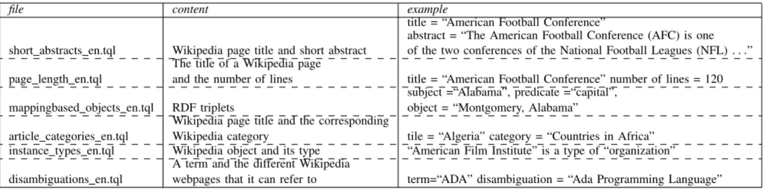
Wikipedia contains information about our world. This in-cludes information about people, organizations, movies, songs, and places, where most of this information is not part of WordNet. DBPedia [20] contains structured information that is extracted from Wikipedia. Specifically, we incorporate in-formation from the six files that are shown in Table II. The information in the files uses the Turtle (Terse RDF Triple Language) syntax.
Our algorithm first creates a node for every Wikipedia article and category. The label of the node will be the title of the Wikipedia article or Wikipedia category (i.e., either wt for Wikipedia title, wc for Wikipedia category). The information about the Wikipedia titles and categories can be extracted from the article categories en.tql file. This differs from our approach in [38] where we store no meta information.
Table III shows the formulas for computing the probabilities based on information from DBPedia. The coefficients for DB-Pedia are in general smaller than those for WordNet because the later contains information of higher quality. Fine-tuning these coefficients remains an area for future research.
Consider the Wikipedia page with title “National Hockey League”. We will create the following formula.
The number 0.25 is computed as 0.4 ∗ norm(1/3) be-cause there are three words in the Wikipedia title. We will create similar formulas between “National Hockey League” and “hockey” and “league”. Note that if “National Hockey League” was a word form in WordNet, then we create a single formulas as follows: [nationalhockeyleague,wt] ⇒ [nationalhockeyleague,wf noun],0.4∗norm(1) = 0.48. The idea of the formula is to connect the nodes from WordNet and DBPedia. Note that the formula applies to both Wikipedia titles and Wikipedia categories.
Next, consider the information that the Wikipedia article “Algeria” corresponds to the Wikipedia category “Countries in Africa”. We create the following formula.
The example assumes that the Wikipedia page for Algeria has 400 lines and the total number of lines of all Wikipedia pages in the category “Countries in Africa” is 10,000. The idea of the formula is that if there were only few Wikipedia pages in a category, then the relationship between the Wikipedia page and category would be stronger.
Next, consider the information that the capital of Alabama is Montgomery. We create the following formula.
The example assumes that there are 20 different RDF triplets where Alabama is the subject. The idea is that the if Alabama has only few RDFs where it is the subject, then we give higher importance to these relations.
Next, consider the DBPedia information that “chair” is a type of “furniture”. We will create the following formula.
The formula assumes that the Wikipedia page for “chair” has 100 lines, while the number of lines of all Wikipedia things that are of type furniture is 1000. The formulas tries to estimate what percent of furniture refers to chairs, that is, what is the probability that someone who is interested in furniture is also interested to know more about chairs.
Next, consider the example that one disambiguation of “ADA” is “Ada Programming Language”. We create the fol-lowing formula.
The formula assumes that there are a total of 40 different disambiguations of ADA. The idea of the formula is that if there are only few disambiguations, then the strength of the relationship between the disambiguation page concept and each of the disambiguation artifacts is stronger.
In order to save space, we do not show examples of the reverse relationships from Table III.
C. Computing the Edge Weights
So far, we have created the nodes of the graph and shown formulas that contain conditional probabilities between nodes. For example, the formula
[X]⇒[Y], p
means that if we are interested in X, then we are also interested in Y with probability p. We will adopt the Markov Logic Network [29] model and rewrite the formula as a first order formula with probability, where the predicate rel tells us whether or not the concept is relevant to the user.
rel(X)⇒rel(Y), p
Next, suppose that the formulas from Tables I and III generate one ore more formulas between the nodes X and
Y. We first convert each probability to a MLN weight using the formula.
(
Note that we first transform the probability in the range [0.5,1] because we want each formula to contribute positively to the weight. In other words, p0 = 0.5 +p2. We then apply the MLN model that computes the weight of a formula as the
p
natural logarithm of the odds, or w =ln( 00) =ln( 1+p).
1−p 1−p An extreme case is when p= 1and the weight will be equal to infinity. We address this case by setting the weight equal to 9.9034 when the probability is too high.
e −1
p=
ew+ 1 w
file content example
title = “American Football Conference”
abstract = “The American Football Conference (AFC) is one short abstracts en.tql Wikipedia page title and short abstract of the two conferences of the National Football Leagues (NFL) ...”
The title of a Wikipedia page
page length en.tql and the number of lines title = “American Football Conference” number of lines = 120 subject =“Alabama”, predicate =“capital”,
mappingbased objects en.tql RDF triplets object = “Montgomery, Alabama” Wikipedia page title and the corresponding
article categories en.tql Wikipedia category tile = “Algeria” category = “Countries in Africa” instance types en.tql Wikipedia object and its type “American Film Institute” is a type of “organization”
A term and the different Wikipedia
disambiguations en.tql webpages that it can refer to term=“ADA” disambiguation = “Ada Programming Language”
count(w,d) [d]⇒[w],norm( ) |d| m [w]⇒[d],log2( ) docFr(w) TABLE II FILES FROM WIKIPEDIA
TABLE III
THE DIFFERENT FORMULAS FOR MODELING DBPEDIA
type from to
Wikipedia title t word win Wikipedia title 0.4
title ∗ probability count(w,t) norm( P count(wi,t) wi∈t )
word w Wikipedia title tthat contains w 0.2
dtf[1](w)
Wikipedia page t word wthat appears in the abstract aof tthree or more times 0.2
abstract
∗norm( Pcount(w,a) count(wi,a) [2]
wi∈frequent3 (a)
)
word w Wikipedia page tthat contains w3 or more times in the abstract 0.1
daf[3](w)
Wikipedia category c Wikipedia article tthat belongs to the category category
Wikipedia article t Wikipedia category c, where tbelongs to c
0.6∗|t|[4] P |ti| ti∈c 0.1 cf[5](t)
subject sof RDF triplet object oof RDF triplet RDF triplet
object oof RDF triplet subject sof RDF triplet
sf of 0.2 [6](s) 0.2 [7](s)
type t object othat belongs to t
instance
0.8∗|o|
P
|oi| oi∈t
object o type t, where obelongs to t 0.1
tf[8](o)
disambiguation page d article tthat is one of the disambiguations
df disambiguation Wikipedia article t disambiguation page dthat points to t
0.8 [9](d)
0.1
.[1]dtf stands for document title frequency. dtf(w)returns the number of documents that contain the word win their title. .[2]frequent
3(s)returns the number of words that occur three or more times in the string s.
.[3]daf stands for document abstract frequency. daf(w)returns the number of documents that contain the word w in their abstract three or more times. .[4]|t|returns the number of lines in the Wikipedia article t.
.[5]cf stands for category frequency. cf(t)returns the number of categories that tbelongs to. .[6]sf stands for subject frequency. sf(s)returns the number of RDF triplets that have subject s. .[7]of stands for object frequency. of(o)returns the number of RDF triplets that have object o. .[8]tf stands for type frequency. tf(t)returns the number of types that tbelongs to.
.[9]df stands for disambiguation frequency. df(d)returns the number of disambiguations for the disambiguation page d.
Next, if there are multiple formulas between two nodes, we follow the MLN model and just add the weights. Finally, we convert the total weight back to probability using the reverse d
IV. CLUSTERING THE DOCUMENTS
We add each document as a node in the graph. Consider a ocument dand a word form w in the document. We create
formula. the following formula.
In the formula, count(w,d)denotes the number of times the We create an edge between every two nodes that participate word form appears in the document and |d|denotes the total in a formula, where the weight of the edge will be computed number of words in the document.
using the above formula. As a last step, we normalize the We also create a formula for the reverse relationship. weights of the edges so that the sum of the weights of the
P r(d1|d2) +P r(d2|d1)
distance(d1, d2) =
2
The function docFr(w) returns the number of documents that contain the word w and m is the total number of documents. Both formulas are similar to the abstract formula from Table III. The reason is that we can think of the abstract of a Wikipedia article as the text of a document. As explained in [39], this formula allows us to compute the distance between two documents in a way that is similar to normalizing the document vectors using the TF-IDF function [16] and then using the cosine distance formula.
Next, we create an edge in the graph for each formula, where we will normalize the weights again to make sure that the sum of the weights of the outgoing edges for every node is equal to 1. Note that we did not have to convert the probabilities to MLN weights in this step because we do not create duplicate edges.
Given two nodes Xand Y in the graph, we define P r(X|Y)
as the conditional probability that X is relevant given that Y
is relevant. This number can be estimated, for example, by doing multiple random walks starting at Y and calculating the percent that reach X [36]. Since the sum of the weights of the outgoing edges is always 1, at each node we can randomly decide where to hop next. For example, if we are at a node
n and there is an outgoing edge to n1 with weight w1, to
n2 with weight w2 and to n3 with weight w3, then we can
generate a random number between 0 and 1. If the number is smaller or equal to w1, then we will hop to n1. If the number
is between w1and w1+w2, then we will hop to n2. Otherwise,
we will hop to n3. When conducting random walks, we only
have to be careful not to revisit the same node multiple times. In particular, our algorithm keeps a hash table of visited nodes and always looks for a path that does not involve nodes that are already visited. We also apply the bounded box techniques from [36] to make the calculations efficient.
Given two documents d1 and d2, we compute the distance
between them using the formula.
We use the k-means clustering algorithm [21] to classify the documents. The algorithm starts with k document seeds. It then finds the documents that are closest to each seed using the distance metric. Next, the centroid (i.e., mean) of each cluster is found and then new clusters are created using the centroids as the seeds. The process repeats and it is guaranteed to converge. Computing the mean of a set of documents amounts to adding the document vectors and dividing by the number of documents. The document vector for a document contains the frequency of each word in the document.
V. EXPERIMENTAL VALIDATION
We used a Hadoop cluster of seven computers running Intel(R) Xeon(R) CPU E5-2695 v3 @ 2.30GH 14 cores and 32 GB RAM to run the experiments. All code was written in Scala and used Spark. Information from WordNet using the Java API for WordNet Searching (JAWS) [34] was first extracted and saved to files. We did not use any search structures, such as
TABLE IV
RESULTS ON THE REUTERS-21578 BENCHMARK
cosine logarithmic this paper
# of rounds 30 45 49
precision 0.57 0.66 0.71
recall 0.05 0.07 0.14
F1-measure 0.09 0.13 0.23
hash tables and trees. Instead, we used Spark’s join operation when we wanted to join the result of two Resilient Distributed Datasets (RDDs). It took less than one hour to create the probabilistic graph using the files for WordNet and DBPedia. We next read all the documents from the Reuters-21578 benchmark. The benchmark contains 21,578 documents that are stored in 22 text files. Our program read the files and we extracted information about the 11,362 documents that were classified in one of 82 categories using human judgment (the other documents do not have human judgment associated with them). For every document, we stored its title, its text, the category it belongs to, and a document vector. The later contains the non-noise words in the document and their frequencies. Since the words in the title are more important, we counted these words twice. We next added the documents to the probabilistic graph.
We next clustered the documents using the k-means clus-tering algorithm. We chose the value k = 82 because this is the number of categories as determined by the human judgment. The first 82 documents were put in 82 distinct clusters. At this point, the lonely document in each category was designed as the centroid. We next processed the rest of the documents. Every document was compared to the 82 centroids and assigned to the cluster with the closest centroid. Next, a new centroid was chosen for each cluster. This was done by adding the document vectors in each cluster and dividing the result by the number of vectors. Next, the documents were reclustered around the new centroids and the process was repeated until it converged.
The k-means clustering algorithm is based on two document functions: finding the distance between two documents and computing the average of several documents. We have three choices for the distance metric: the standard cosine function, the logarithmic function from [41] that uses only information from WordNet, and the random walk function on the full probabilistic graph that stores information from WordNet and DBPedia.
Table IV shows the F1-measure when using the three
different distance metrics. The measure gives a single number based on the precision and recall of the result of the clustering
TP
algorithm. We computed the precision as TP+FP and the TP
recall as TP+FN. In the formula, TP is the number of true positives, that is, the number of documents that were classified in the same category by both the program and human judgment. FP is the number of false positives, that is, the number of documents that were classified in the same category by the program, but were classified in different categories by
human judgment. Lastly, FN is the number of false negatives, that is, the number of documents that were classified in the same category by human judgment but were classified in different categories by the program.
As the table suggests, using the full probabilistic graph with information from WordNet and DBPedia can lead to both higher precision and recall. The reason is that now we are not just comparing the semantic similarity between words, but also the semantic similarity between phrases.
VI. CONCLUSION AND FUTURE RESEARCH In this paper, we reviewed how information from WordNet can be used to build a probabilistic graph. We extended existing algorithms by adding part of speech tag to each word and sense. We then showed how the graph can be extended with information from DBPedia. We validated the algorithm experimentally by comparing it to an algorithm that uses the cosine similarity metric and an algorithm that uses only information from WordNet. The results show that adding information from DBPedia increases both the precision and the recall of the algorithm on the Reuters-21578 benchmark.
One area for future research is moving beyond the bag of words model and considering the ordering of the words in the documents.
REFERENCES
[1] M. Agosti and F. Crestani. Automatic Authoring and Construction of Hypertext for Information Retrieval. ACM Multimedia Systems, 15(24), 1995.
[2] M. Agosti, F. Crestani, G. Gradenigo, and P. Mattiello. An Approach to Conceptual Modeling of IR Auxiliary Data. IEEE International Conference on Computer and Communications, 1990.
[3] L. Burnard. Reference Guide for the British National Corpus (XML Edition). http://www.natcorp.ox.ac.uk, 2007.
[4] P. Cohen and R. Kjeldsen. Information Retrieval by Constrained Spreading Activation on Sematic Networks. Information Processing and Management, pages 255–268, 1987.
[5] R. Collobert and J. Weston. A Unified Architecture for Natural Language Processing: Deep Neural Networks with Multitask Learning. Twenty Fifth International Conference on Machine Learning, 2008.
[6] F. Crestani. Application of Spreading Activation Techniques in Infor-mation Retrieval. Artificial Intelligence Review, 11(6):453–482, 1997. [7] Croft. User-specified Domain Knowledge for Document Retrieval.
Nineth Annual International ACM Conference on Research and Devel-opment in Information Retrieval, pages 201–206, 1986.
[8] S. Deerwester, S. T. Dumais, G. W. Furnas, T. K. Landauer, and R. Harshman. Indexing by Latent Semantic Analysis. Journal of the Society for Information Science, 41(6):391–407, 1990.
[9] C. Fox. Lexical Analysis and Stoplists. Information Retrieval: Data Structures and Algorithms, pages 102–130, 1992.
[10] W. Frakes. Stemming Algorithms. Information Retrieval: Data Struc-tures and Algorithms, pages 131–160, 1992.
[11] T. Gruber. Collective knowledge systems: Where the social web meets the semantic. Web Journal of Web Semantics, 2008.
[12] R. V. Guha, R. McCool, and E. Miller. Semantic Search. Twelfth International World Wide Web Conference (WWW 2003), pages 700– 709, 2003.
[13] E. H. Hovy, L. Gerber, U. Hermjakob, M. Junk, and C. Y. Lin. Question Answering in Webclopedia. TREC-9 Conference, 2000.
[14] K. Jarvelin, J. Keklinen, and T. Niemi. ExpansionTool: Concept-based Query Expansion and Construction. Springer Netherlands, pages 231– 255, 2001.
[15] G. Jeh and J. Widom. SimRank: A Measure of Structural-context Similarity. Proceedings of the Eight ACM SIGKDD International Conference on Knowledge Discovery and Data Mining, pages 538–543, 2002.
[16] K. Jones. ”a statistical interpretation of term specificity and its applica-tion in retrieval”. Journal of Documentation, 28(1):11–21, 1972. [17] A. Kiryakov, B. Popov, I. Terziev, D. Manov, and D. Ognyanoff.
Se-mantic Annotation, Indexing, and Retrieval. Journal of Web Semantics, 2(1):49–79, 2004.
[18] R. Knappe, H. Bulskov, and T. Andreasen. Similarity Graphs. Fourteenth International Symposium on Foundations of Intelligent Systems, 2003. [19] T. K. Landauer, P. Foltz, and D. Laham. Introduction to Latent Semantic
Analysis. Discourse Processes, pages 259–284, 1998.
[20] J. Lehmann, R. Isele, M. Jakob, A. Jentzsch, D. Kontokostas, P. N. Mendes, S. Hellmann, M. Morsey, P. van Kleef, S. Auer, and C. Bizer. DBpedia A large-scale, multilingual knowledge base extracted from Wikipedia. Semantic Web, 6(2):167–195, 2015.
[21] J. B. MacQueen. Some Methods for Classification and Analysis of Multivariate Observations. Proceedings of Fifth Berkeley Symposium on Mathematical Statistics and Probability, pages 281–297, 1967. [22] C. D. Manning, M. Surdeanu, J. Bauer, J. Finkel, S. J. Bethard, and
D. McClosky. The Stanford CoreNLP natural language processing toolkit. In Association for Computational Linguistics (ACL) System Demonstrations, pages 55–60, 2014.
[23] M.F.Porter. An Algorithm for Suffix Stripping. Readings in Information Retrieval, pages 313–316, 1997.
[24] T. Mikolov, K. Chen, G. Corrado, and J. Dean. Efficient Estimation of Word Representations in Vector Space. arXiv:1301.3781.
[25] G. A. Miller. WordNet: A Lexical Database for English. Communica-tions of the ACM, 38(11):39–41, 1995.
[26] D. Moldovan, S. Harabagiu, M. Pasca, R. Mihalcea, R. Goodrum, and R. Girju. LASSO: A Tool for Surfing the Answer Net. Text Retrieval Conference (TREC-8), 1999.
[27] B. Popov, A. Kiryakov, D. D. Ognyanoff, D. Manov, and A. Kirilov. KIM A Semantic Platform for Information Extraction and Retrieval. Journal of Natural Language Engineering, 10(3):375–392, 2004. [28] L. Rau. Knowledge Organization and Access in a Conceptual
Informa-tion System. Information Processing and Management, 23(4):269–283, 1987.
[29] M. Richardson and P. Domingos. Markov Logic Networks. Machine Learning, 62(1-2):107–136, 2006.
[30] M. Sanderson. Word Sense Disambiguation and Information Retrieval. Seventeenth annual international ACM SIGIR conference on Research and development in information retrieval, 1994.
[31] P. Shoval. Expert consultation system for a retrieval database with semantic network of concepts. Fourth Annual International ACM SIGIR Conference on Information Storage and Retrieval: Theoretical Issues in Information Retrieval, pages 145–149, 1981.
[32] Simone Paolo Ponzetto and Michael Strube. Deriving a Large Scale Taxonomy from Wikipedia. 22nd International Conference on Artificial Intelligence, 2007.
[33] E. Sirin and B. Parsia. SPARQL-DL: SPARQL Query for OWL-DL. OWL: Experiences and Directions Workshop, 2007.
[34] B. Spell. Java API for WordNet Searching (JAWS). http://lyle.smu.edu/ tspell/jaws/index.html, 2009.
[35] K. Srihari, W. Li, and X. Li. Information Extraction Supported Question Answering. In Advances in Open Domain Question Answering, 2004. [36] L. Stanchev. Implementing Semantic Document Search Using a
Bounded Random Walk in a Probabilistic Graph. IEEE International Conference of Semantic Computing, 2008.
[37] L. Stanchev. Building Semantic Corpus from WordNet. The First International Workshop on the role of Semantic Web in Literature-Based Discovery, 2012.
[38] L. Stanchev. Creating a Phrase Similarity Graph from Wikipedia. Eight IEEE International Conference on Semantic Computing, 2014. [39] L. Stanchev. Fine-Tuning an Algorithm for Semantic Search Using
a Similarity Graph. International Journal on Semantic Computing, 9(3):283–306, 2015.
[40] L. Stanchev. Creating a Probabilistic Graph for WordNet using Markov Logic Network. Proceedings of the Sixth International Conference on Web Intelligence, Mining and Semantics, pages 1–12, 2016.
[41] L. Stanchev. Semantic Document Clustering Using a Similarity Graph. Tenth IEEE International Conference on Semantic Computing, pages 1–8, 2016.
[42] J. Turian, L. Ratinov, and Y. Bengio. Word representations: A simple and general method for semi-supervised learning. In Forty Eight Anual Meeting of the Association for Computational Linguistics, pages 384– 394, 2010.