shallow networks?
Bernd
Illing
a,∗,
Wulfram
Gerstner
aand
Johanni
Brea
aaBrain Mind Institute, EPFL, 1015 Lausanne, Switzerland
A R T I C L E I N F O
Keywords: Deep learning Local learning rules Random Projections
Unsupervised Feature Learning Spiking Networks
MNIST CIFAR10
A B S T R A C T
Training deep neural networks with the error backpropagation algorithm is considered implausible from a biological perspective. Numerous recent publications suggest elaborate models for biologi-cally plausible variants of deep learning, typibiologi-cally defining success as reaching around 98% test ac-curacy on the MNIST data set. Here, we investigate how far we can go on digit (MNIST) and object (CIFAR10) classification with biologically plausible, local learning rules in a network with one hid-den layer and a single readout layer. The hidhid-den layer weights are either fixed (random or random Gabor filters) or trained with unsupervised methods (Principal/Independent Component Analysis or Sparse Coding) that can be implemented by local learning rules. The readout layer is trained with a supervised, local learning rule. We first implement these models with rate neurons. This compari-son reveals, first, that unsupervised learning does not lead to better performance than fixed random projections or Gabor filters for large hidden layers. Second, networks with localized receptive fields perform significantly better than networks with all-to-all connectivity and can reach backpropagation performance on MNIST. We then implement two of the networks - fixed, localized, random & ran-dom Gabor filters in the hidden layer - with spiking leaky integrate-and-fire neurons and spike timing dependent plasticity to train the readout layer. These spiking models achieve > 98.2% test accuracy on MNIST, which is close to the performance of rate networks with one hidden layer trained with backpropagation. The performance of our shallow network models is comparable to most current biologically plausible models of deep learning. Furthermore, our results with a shallow spiking net-work provide an important reference and suggest the use of datasets other than MNIST for testing the performance of future models of biologically plausible deep learning.
1. Introduction
While learning a new task, synapses deep in the brain undergo task-relevant changes [1]. These synapses are of-ten many neurons downstream of sensors and many neu-rons upstream of actuators. Since the rules that govern such changes deep in the brain are poorly understood, it is appeal-ing to draw inspiration from deep artificial neural networks (DNNs) [2]. DNNs and the cerebral cortex share that infor-mation is processed in multiple layers of many neurons [3,4] and that learning depends on changes of synaptic strengths [5]. However, learning rules in the brain are most likely dif-ferent from the backpropagation algorithm [6,7,8]. Further-more, biological neurons communicate by sending discrete spikes as opposed to real-valued numbers used in DNNs. Differences like these suggest that there exist other, possibly nearly equally powerful, algorithms that are capable to solve the same tasks by using different, more biologically plausi-ble mechanisms. Thus, an important question in computa-tional neuroscience is how to explain the fascinating learn-ing capabilities of the brain with biologically plausible net-work architectures and learning rules. Moreover from a pure machine learning perspective there is increasing interest in neuron-like architectures with local learning rules, mainly motivated by the current advances in neuromorphic hard-ware [9].
Image recognition is a popular task to test the performance of
∗Corresponding author
[email protected](B. Illing) ORCID(s):
neural networks. Because of its relative simplicity and popu-larity, the MNIST dataset (28×28-pixel grey level images of handwritten digits, LeCun [10]) is often used for benchmark-ing. Typical performances of existing models are around 97-99% classification accuracy on the MNIST test set (see sec-tion 2andTable 1). Since the performances of many classi-cal DNNs trained with backpropagation (but without data augmentation or convolutional layers, see table in LeCun [10]) also fall in this region, accuracies around these values are assumed to be an empirical signature of backpropagation-like deep learning [11,12,13,8]. It is noteworthy, however, that several of the most promising approaches that perform well on MNIST have been found to fail on harder tasks [14] or at least need major modifications to scale to deeper net-works [15].
There are two obvious alternatives to supervised training of all layers with backpropagation. The first one is to fix weights in the first layer(s) at random values , as proposed by general approximation theory [16] and the extreme learning field [17]. The second alternative is unsupervised training in the first layer(s). In both cases, only the weights of a readout layer are learned with supervised training. Unsupervised methods are appealing since they can be implemented with local learning rules, see e.g. “Oja’s rule” [18,19] for princi-pal component analysis, nonlinear extensions for indepen-dent component analysis [20] or algorithms in Olshausen and Field [21], Rozell et al. [22], Liu and Jia [23], Brito and Gerstner [24] for sparse coding. A single readout layer can be implemented with a local rule as well. A candidate is the delta-rule (also called “perceptron rule”), which may be
implemented by pyramidal spiking neurons with dendritic prediction of somatic spiking [25]. Since straightforward stacking of multiple fully connected layers of unsupervised learning does not reveal more complex features [21] we fo-cus here on networks with a single hidden layer (see also Krotov and Hopfield [26]).
The main objective of this study is to see how far we can go with networks with a single hidden layer and biologi-cally plausible, local learning rules, preferably using spiking neurons. To do so we first compare the classification per-formance of different rate networks: networks trained with backpropagation, networks with fixed random projections or random Gabor filters in the hidden layer and networks where the hidden layer is trained with unsupervised meth-ods (section 4). Since sparse connectivity is sometimes su-perior to dense connectivity [27,14] and successful convo-lutional networks leverage local receptive fields, we inves-tigate sparse connectivity between input and hidden layer, where each hidden neuron receives input only from a few neighboring pixels of the input image (section 5). Finally we implement the simplest, yet promising and biologically plau-sible models - localized random projections and random Ga-bor filters - with spiking leaky integrate-and-fire neurons and spike timing dependent plasticity (section 6). We discuss the performance and implications of this simplistic model with respect to current models of biologically plausible deep learning.
2. Related work
In recent years, many biologically plausible approaches to deep learning have been proposed, see e.g. Marblestone et al. [7], Whittington and Bogacz [8], Tavanaei et al. [13] for reviews. Existing approaches usually use either involved architectures or elaborate mechanisms to approximate the backpropagation algorithm. Examples include the use of convolutional layers [28,13, 29, 30] (and tables therein), dendritic computations [31,32,12] or backpropagation ap-proximations such as feedback alignment [11,33,34,35,36, 14] equilibrium propagation [37], membrane potential based backpropagation [38], restricted Boltzmann machines and deep belief networks [39,40], (localized) difference target propagation [41,14], using reinforcement-signals [42,43] or approaches using predictive coding [44]. Many models implement spiking neurons to stress bio-plausibility [45,46, 47,48,49,13] (and tables therein) or coding efficiency [50]. The conversion of DNNs to spiking neural networks (SNN) after training with backpropagation [51] is a common tech-nique to evade the difficulties of training with spikes. Fur-thermore, there are models including recurrent activity [52, 53], starting directly from realistic circuits [54], or combin-ing unsupervised and supervised traincombin-ing [26] as in this pa-per. We refer toTable 1for an extensive list of current bio-logically plausible models tested on MNIST.
3. Results
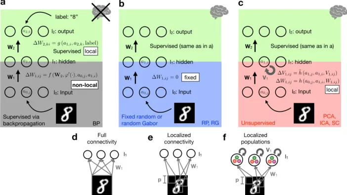
We study networks that consist of an input (𝑙0), one hid-den (𝑙1) and an output-layer (𝑙2) of (nonlinear) units, con-nected by weight matricesW1andW2(Figure 1). Training the hidden layer weightsW1with standard supervised train-ing involves (non-local) error backpropagation ustrain-ing sum-mation over output units, the derivative of the units’ non-linearity (𝜑′(⋅)) and the transposed weight matrixW𝑇2 ( Fig-ure 1a). In the biologically plausible network considered in this paper (Figure 1b & c), the input-to-hidden weights W1are either fixed random, random Gabor filters or learned with an unsupervised method (Principal/ Independent Com-ponent Analysis or Sparse Coding). The unsupervised learn-ing algorithms assume recurrent inhibitory weightsV1 be-tween hidden units to implement competition, i.e. to make different hidden units learn different features. For more model details we refer toAppendix A-Appendix D.
4. Benchmarking biologically plausible rate
models and backpropagation
To see how far we can go with a single hidden layer, we systematically investigate rate models using different meth-ods to initialize or learn the hidden layer weightsW1(see Figure 1and methodsAppendix A-Appendix Cfor details). We use two different ways to set the weightsW1of the hid-den layer: either using fixed Random Projections (RP) or Random Gabor filters (RG), seeFigure 1b & blue curves in Figure 2, or using one of the unsupervised methods Prin-cipal Component Analysis (PCA), Independent Component Analysis (ICA) or Sparse Coding (SC), seeFigure 1c & red curves inFigure 2. All these methods can be implemented with local, biologically plausible learning rules [18,20,21]. We refer to the methodsAppendix Bfor further details. As a reference, we train networks with the same architecture with standard backpropagation (BP, seeFigure 1a). As a step from BP towards increased biologically plausibility, we include Feedback Alignment (FA, Lillicrap et al. [11]) with fixed random feedback weights for error backpropagation (see methodsAppendix Dfor further explanation). A Sim-ple Perceptron (SP) without a hidden layer serves as a fur-ther reference, since it corresponds to direct classification of the input. We expect any biologically plausible learning al-gorithm to achieve results somewhere between SP (“lower”) and BP (“upper performance bound”)
The hidden-to-output weightsW2are trained with standard stochastic gradient descent (SGD), using a one-hot represen-tation of the class label as target. Since no error backpropa-gation is needed for a single layer, the learning rule is local (“delta” or “perceptron”-rule). Therefore the two-layer net-work as a whole is biologically plausible in terms of online learning and synaptic updates using only local variables. For computational efficiency, we first train the hidden layer and then the output layer, however, both layers could be trained simultaneously.
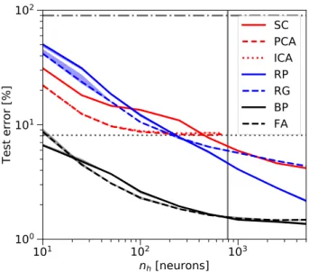
We compare the test errors on the MNIST digit recognition data set for varying numbers of hidden neurons𝑛ℎ(Figure 2). The PCA (red dashed) and ICA (red dotted) curves in
b
Unsupervised l0: Input l1: hidden l2: output W1 W2 V1 l0: Input l1: hidden l2: output W1 W2a
label: “8” W1 Full connectivity l1c
d
e
l1 Localized connectivity p W1 Localized populations l1 W1 V1 Fixed random or random Gabor l0: Input l1: hidden l2: output W1 W2f
a0,j a1,i a2,k W1,ij=f(W2, '0(·), a0,j, a1,i) (nonlocal) a0,j a1,i a0,j a1,iW1,ij=h(a0,j, a1,i, W1,ij)
(local)
V1,ij= ˜h(a1,j, a1,i, V1,ij) W1,ij= 0 (fixed)
W2,ki=g(a1,i, a2,k,label)
(local) Supervised Supervised via backpropagation p Supervised (same as in a) BP RP, RG PCA, ICA, SC non-local local fixed local Supervised (same as in a)
Figure 1: The proposed network model has one hidden layer (𝑙1) and one readout layer (𝑙2) of nonlinear units (nonlinearity𝜑(⋅)). Respective neural activations (e.g. 𝑎0,𝑗) and update rules (e.g. Δ𝑊1,𝑖𝑗) are added. (𝑓(⋅))𝑔(⋅), ℎ(⋅)& ̃ℎ(⋅)are (non-)local plasticity functions, i.e. using only variables (not) available at the synapse for the respective update. a Training with backpropagation (BP) through one hidden layer is biologically implausible since it is nonlocal (e.g. usingW2 &𝜑′(⋅)from higher layers to update
W1, seeAppendix D). b&cBiologically plausible architecture with fixed Random Projections (RP) or fixed random Gabor filters (RG) (blue box inb) or unsupervised feature learning in the first layer (red box inc), and a supervised classifier in the readout layer𝑙2(green boxes). All weight updates are local. Wstands for feed-forward,Vfor recurrent, inhibitory weights. (Crossed out) brain icons in a,b & c stand for (non-)bio-plausibility of the whole network. d &eIllustration of fully connected and localized receptive fields ofW1. f For localized Principal/Independent Component Analysis (𝑙-PCA/𝑙-ICA) and Sparse Coding (𝑙-SC) the hidden layer is composed of independent populations. Neurons within each population share the same localized receptive field and compete with each other while the populations are conditionally independent. For more model details, seeAppendix A -Appendix D.
ure 2end at the vertical line𝑛ℎ=𝑑= 784because the num-ber of principal/independent components (PCs/ICs), i.e. the number of hidden units𝑛ℎ, is limited by the input dimension
𝑑. Since the PCs span the subspace of highest variance, clas-sification performance quickly improves when adding more PCs for small𝑛ℎand then saturates for larger𝑛ℎ. ICA does not seem to discover significantly more useful features than PCA, leading to similar classification performance. SC (red solid line) extracts sparse representations that can be overcomplete (𝑛ℎ > 𝑑), leading to a remarkable classifi-cation performance of around 96 % test accuracy. This sug-gests that the sparse representation and the features extracted by SC are indeed useful for classification, especially in the overcomplete case.
As expected, the performance of RP (blue solid) for small numbers of hidden units (𝑛ℎ < 𝑑) is worse than for feature extractors like PCA, ICA or SC. Also for large hidden lay-ers, performance improves only slowly with𝑛ℎ, which is in line with theory [16] and findings in the extreme learning field [17]. However, for large hidden layers sizes, RP out-performs SC.
As a reference, we also studied fixing the hidden layer weights to Gabor filters of random orientation, phase and size, lo-cated at the image center (RG, blue dashed, seeAppendix C). For hidden layers with more than 1000 neurons, SC is only marginally better than the network with fixed random Gabor filters.
For all tested methods and hidden layer sizes, perfor-mance is significantly worse than the one reached with BP (black solid inFigure 2). In line with [11], we find that FA (black dashed) performs as well as BP on MNIST. Universal function approximation theory predicts lower bounds for the squared error that follow a power law with hidden layer size
𝑛ℎfor both BP ((1∕𝑛ℎ)) and RP ((1∕𝑛2∕ℎ 𝑑), where𝑑is the input dimension [60,16]). In the log-log-plot inFigure 2this would correspond to a factor𝑑∕2 = 784∕2 = 392between the slopes of the curves of BP and RP, or at least a factor
𝑑eff∕2 ≈ 10 using an effective dimensionality of MNIST (see methodsA). We find a much faster decay of classifica-tion error in RP and a smaller difference between RP and BP slopes than suggested by the theoretical lower bounds. Taken together, these results show that the high
dimension-Table 1
MNIST benchmarks for biologically plausible models of deep learning compared with mod-els in this paper (bold). SNN: Spiking Neural Network, for other abbreviations seesection 3. Models are ranked by MNIST test accuracy (rightmost column). Parts of this table are taken from [13,30,55]. Models using convolutional layers (CNN) are marked inorange. For conventional ANN/DNN/CNN MNIST benchmarks seetablein [10].
Model Neural coding Learning type Comments Test accuracy (%)
Conv. SNN [48] Spikes Supervised 5 conv. layers, Spatio-Temporal BP 99.3 Conv. SNN [51] Rate Supervised Conversion: rate→spike 99.1 Conv. Spiking AE[56] Spikes Un/Supervised Stacked conv. AE with BP + sym. weights 99.1 𝑙-RG(this paper) Rate Un/Supervised Only output layer learned 98.9
𝑙-BP(this paper) Rate Supervised BP-benchmark of this paper 98.8
𝑙-ICA(this paper) Rate Un/Supervised ICs as features for SGD 98.8
𝑙-FA[14] (& this paper) Rate Supervised FA with localized rec. fields 98.7
SNN [38] Spikes Supervised BP approx., weight symmetry 98.7
spiking LIF𝑙-RG(this paper) Spikes Supervised STDP (only output layer learned) 98.6
(Stoch.) Diff. Target Prop. [41] Rate Supervised Layer-wise AE, Target Prop. 98.5 Nonlin. Hebb + SGD [26] Rate Un/Supervised nonlin. Hebb + SGD (similar to this paper) 98.5
𝑙-RP(this paper) Rate Supervised Only output layer learned 98.4
𝑙-SC(this paper) Rate Un/Supervised SC for 1. layer, SGD for 2. layer 98.4
Conv. SNN [30] Spikes Unsupervised 3 Conv. layers, STDP, ext. SVM 98.4 SNN [50] Pseudo-spike Supervised Sparse, discrete activities, STDP 98.3
Direct FA [34] Rate Supervised Many hidden layers 98.3
Spiking FA [11] Spikes Supervised 3 hidden layers 98.2
spiking LIF𝑙-RP(this paper) Spikes Supervised STDP (only output layer learned) 98.2
𝑙-PCA(this paper) Rate Un/Supervised PCs as features for SGD 98.2
Q-AGREL (RL-like) [43] Rate RL-like RL-like BP-approx. 98.2
Forward propagation (FP) [36] Rate Supervised FP: BP approximation 98.1
Spiking FA [46] Spikes Supervised Direct FA 98
Predictive coding [44] Rate Supervised BP approx. by pred. coding 98 Spiking CNN [28] Rate/Spikes Unsupervised Semi-online, STDP, ext. SVM 98 Equilibrium Prop. [37] Rate Supervised 1 - 3 hidden layers 97 - 98
Dendr. BP [12] Spikes Supervised Dendr. comp. for BP approx. 97.5
Spiking FA [35] Spikes Supervised 3 hidden layers 97
Sparse/Skip FA [33] Rate Supervised Sparse- & Skip-FA 96 - 97 Spiking CNN [57] Spikes Unsupervised Recurrent Inhib., STDP 96.6
Spiking FA [32] Spikes Supervised Dendr. comp. for BP approx. 96.3 2 layer network [55] Spikes Unsupervised Recurrent Inhib., purely unsuperv. 95 Spiking RBM/DBN [39] Rate Supervised Conversion rate→spike 94.1
2 layer network [58] Spikes Unsupervised Memristive device 93.5
Spiking HMAX/CNN [49] Spikes Supervised STDP, HMAX preprocess. 93
Spiking RBM/DBN [40] Rate Supervised Neural sampling 92.6
Spiking RBM/DBN [40] Spikes Supervised Neural sampling 91.9
SP(this paper) Rate Supervised Direct classification on MNIST data 91.9
Spiking CNN [59] Spike Supervised Tempotron rule, sensor MNIST 91.3 Dendritic neurons [31] Rate Supervised Nonlin. dendrites, neuromorphic appl. 90.3
ality of the hidden layers is more important for reaching high performance than the global features extracted by PCA, ICA or SC. Tests on the object recognition task CIFAR10 lead to the same conclusion, indicating that this observation is not entirely task specific (seesection 5for further analysis on CIFAR10).
5. Localized receptive fields boost performance
There are good reasons to reduce the connectivity from all-to-all to localized receptive fields (Figure 1e & f): lo-cal connectivity patterns are observed in real neural circuits [61], useful theoretically [27] and empirically [14], and suc-cessfully used in convolutional neural networks (CNNs). Even though this modification seems well justified from both bio-logical and algorithmic sides, it reduces the generality of the algorithm to input data such as images where neighborhood relations between pixels (i.e. input dimensions) areimpor-tant.
To obtain localized receptive fields (called “𝑙-” methods in the following) patches spanning𝑝 ×𝑝 pixels in the input space are assigned to the hidden neurons. The centers of the patches are chosen at random positions in the input space, seeFigure 1e & f. For localized Random Projections (𝑙-RP) and localized random Gabor filters (𝑙-RG) the weights within the patches are randomly drawn from the respective distribu-tion and then fixed. For the localized unsupervised learning methods (𝑙-PCA,𝑙-ICA &𝑙-SC) the hidden layer is split into 500 independent populations. Neurons within each popula-tion compete with each other while different populapopula-tions are independent, seeFigure 1f. This split implies a minimum number of𝑛ℎ= 500hidden neurons for these methods. For
𝑙-PCA and𝑙-ICA a thresholding nonlinearity was added to the hidden layer to leverage the local structure (otherwise
Figure 2: MNIST classification with rate networks according toFigure 1a-c with full connectivity (Figure 1d). The test error decreases for increasing hidden layer size𝑛ℎfor all methods, i.e. Principal/Independent Component Analysis (PCA/ICA, curves are highly overlapping), Sparse Coding (SC), fixed Random Projections (RP) and fixed random Gabor filters (RG) as well as for the fully supervised reference algorithms Backpropaga-tion (BP) and Feedback Alignment (FA). The dash-dotted line at 90 % is chance level, the dotted line around 8 % is the per-formance of a Simple Perceptron (SP) without hidden layer. The vertical line marks the input dimension𝑑 = 784, i.e. the transition from under- to overcomplete hidden representations. Note the log-log scale.
PCA/ICA act globally due to their linear nature, see meth-odsAppendix B).
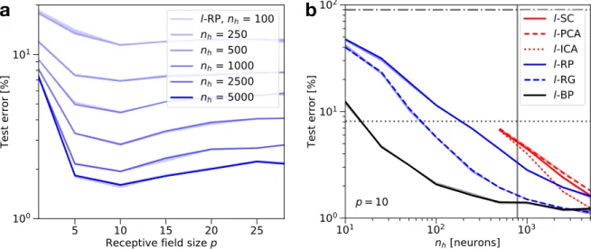
We test𝑙-RP for different patch sizes𝑝and find an optimum around𝑝≈ 10(seeFigure 3a). Note that𝑝= 1corresponds to resampling the data with random weights, and𝑝= 28 re-covers fully connected RP performance. The other methods show similar optimal values around𝑝= 10(not shown). The main finding here is the significant improvement in perfor-mance using localized receptive fields. All tested methods improve by a large margin when switching from full image to localized patches and some methods (𝑙-RG and𝑙-ICA) even reach BP performance for𝑛ℎ = 5000hidden neurons (see Figure 3b). To achieve a fair comparison BP is also imple-mented with localized receptive fields (𝑙-BP) which leads to a minor improvement compared to global BP. This makes lo-cal random projections or lolo-cal unsupervised learning strong competitors to BP as biologically plausible algorithms in the regime of large, overcomplete hidden layers𝑛ℎ> 𝑑- at least for MNIST classification.
To test whether localized receptive fields only work for the relatively simple MNIST data set (centered digits, uninfor-mative margin pixels, no clutter, uniform features and per-spective etc.) or generalizes to more difficult tasks, we apply it to the CIFAR10 data set [62]. We first reproduce a typical benchmark performance of a fully connected network with
one hidden layer trained with standard BP (≈56% test accu-racy,𝑛ℎ = 5000, see also Lin and Memisevic [63]). Again, classification performance increases for increasing hidden layer size𝑛ℎ and localized receptive fields perform better than full connectivity for all methods. Furthermore, as on MNIST, we can see similar performances for local feature learning methods (𝑙-PCA,𝑙-ICA &𝑙-SC) and local random features (𝑙-RP,𝑙-RG) in the case of large, overcomplete hid-den layers (seeTable 2). Also on CIFAR10, localized ran-dom filters and local feature learning reach the performance of biologically plausible models of deep learning [14,26] and come close to the performance of the reference algo-rithm𝑙-BP. However, the difference remains statistically sig-nificant here. Given that the state-of-the-art performance on CIFAR10 with deep convolutional neural networks is close to 98% (e.g. Real et al. [64]), the limitations of our shallow local network and the well-known differences in difficulty between MNIST and CIFAR10 become apparent.
In summary, the main message of this section is that unsu-pervised methods, as well as random features, perform sig-nificantly better when applied locally. Equipped with local receptive fields our shallow network can outperform many current models of biologically plausible deep learning (see Table 1). On MNIST some models (𝑙-RG & 𝑙-ICA) even reach backpropagation performance, while on CIFAR10 large differences to state-of-the-art deep convolutional networks remain.
6. Spiking localized random projections
Real neural circuits communicate with short electrical pulses, called spikes, instead of real numbers such as rates. We thus extend our shallow network model to networks of leaky integrate-and-fire (LIF) neurons. The network archi-tecture is the same as inFigure 1b. To keep it simple we implement the two models with fixed random weights with LIF neurons: fixed localized Random Projections (𝑙-RP) and fixed localized random Gabor filters (𝑙-RG) with patches of size𝑝×𝑝- as insection 5. The output layer weightsW2are trained with a supervised spike timing dependent plasticity (STDP) rule.
7. LIF and STDP dynamics
The spiking dynamics follow the usual LIF equations (see methodsAppendix E) and the readout weightsW2evolve according to a supervised delta rule via spike timing depen-dent plasticity (STDP) using post-synaptic spike-traces tr𝑖(𝑡)
and a post-synaptic target trace tgt𝑖(𝑡)
𝜏tr𝑑tr𝑖(𝑡) 𝑑𝑡 = −tr𝑖(𝑡) + ∑ 𝑓 𝛿 ( 𝑡−𝑡𝑓𝑖 ) (1) Δ𝑤2,𝑖𝑗 = 𝛼⋅ ( tgtpost𝑖 (𝑡) −trpost𝑖 (𝑡) ) 𝛿 ( 𝑡−𝑡𝑓𝑗 ) ,
where 𝛼 is the learning rate. Thus, for a specific readout weight𝑤2,𝑖𝑗, the synaptic trace is updated at every post-synaptic spike time𝑡𝑓𝑖 and the weight is updated at every pre-synaptic spike time𝑡𝑓𝑗. The target trace is constant while a pattern is presented and uses a standard one-hot coding for
b
a
Figure 3:Effect of localized connectivity on MNIST.aTest error for localized Random Projections (𝑙-RP), dependent on receptive field size𝑝for different hidden layer sizes𝑛ℎ. The optimum for receptive field size𝑝= 10 is more pronounced for large hidden layer sizes. Full connectivity is equivalent to𝑝= 28. Note the log-lin scale. bLocalized receptive fields decrease test errors for all tested networks (compareFigure 2): Principal/Independent Component Analysis (𝑙-PCA/𝑙-ICA), Sparse Coding (𝑙-SC), Random Projections (𝑙-RP), Random Gabor filters (𝑙-RG) and Backpropagation (𝑙-BP). The effect is most significant for𝑙-ICA and𝑙-RG, which approach𝑙-BP performance for large𝑛ℎand𝑝= 10, while all other methods reach test errors between1 − 2%. All other reference lines as inFigure 2. 𝑙-PCA/𝑙-ICA &𝑙-SC use 500 independent populations in the hidden layer (seeFigure 1f) which constrains the hidden layer size to𝑛ℎ≥500. Note the log-log scale.
Table 2
Test accuracies (%) on MNIST and CIFAR10 for rate networks and spiking LIF models. The Simple Perceptron (SP) is equivalent to direct classification on the data without hidden layer. All other methods use𝑛ℎ = 5000 hidden neurons and receptive field size𝑝
= 10. Note that CIFAR10 has𝑑 = 32×32×3 = 3072 input channels (the third factor is due to the color channels), MNIST only𝑑= 28×28 = 784. The rate (spiking) models are trained for 167 (117) epochs. Best performing in bold.
SP 𝑙-PCA 𝑙-ICA 𝑙-SC 𝑙-RP 𝑙-RG 𝑙-BP
Rate CIFAR10 35.7±0.7 50.8±0.3 53.9±0.3 50.2±0.2 52.0±0.4 55.6±0.2 58.3±0.2 MNIST 91.9±0.1 98.2±0.02 98.8±0.03 98.4±0.07 98.4±0.1 98.9±0.05 98.8±0.1
Spiking MNIST - 98.2±0.05 98.6±0.1
-the supervisor signal in -the output layer (𝑙2).
To illustrate the LIF and STDP dynamics, a toy example con-sisting of one pre- connected to one post-synaptic neuron is integrated for 650 ms. The pre- and post-synaptic mem-brane potentials show periodic spiking (Figure 4a) which in-duces post-synaptic spike traces and corresponding weight changes (Figure 4b), according toEquation 1. For the MNIST task,Figure 4c shows a raster plot for an exemplary training and testing protocol. During activity transients after a switch from one pattern to the next, learning is disabled until reg-ular spiking is recovered. We experienced that without dis-abling learning during these transient phases the networks never reached a low test error. This is not surprising, since in this phase the network activities carry information both about the previously presented pattern and the current one, but the learning rule is designed for network activities in re-sponse to a single input pattern. It is also known that LIF neurons differ from biological neurons in response to step currents (see Naud et al. [65] and references therein). Dur-ing the testDur-ing period, learnDur-ing is shut off permanently (see
methods sectionEfor more details). The LIF and STDP dy-namics can be mapped to a rate model (see e.g. [51] and Appendix Efor details). However all following results are obtained with the fully spiking LIF/STDP model.
8. Classification results for spiking LIF𝑙-RP
When directly trained with the STDP rule ofEquation 1, the spiking LIF models closely approach the performance of their rate counterparts. Table 2compares the performances of the rate and spiking LIF𝑙-RP &𝑙-RG models with the reference algorithm𝑙-BP (for same hidden layer size𝑛ℎand patch size𝑝, seesection 5). The remaining gap (<0.3%) be-tween rate model and spiking LIF model presumably stems from noise introduced by the spiking approximation of rates and the activity transients mentioned above. Both, the rate and spiking LIF model of𝑙-RP/𝑙-RG achieve accuracies close to the backpropagation reference algorithm𝑙-BP and fall in the range of performance of prominent, biologically plau-sible models, i.e. 98-99% test accuracy (seesection 2and Table 1). Based on these numbers we conclude that the
c
…
106 +
Training
phase
Testing
phase
b
a
Figure 4: Spiking LIF and STDP dynamics. aDynamics of the pre- and postsynaptic membrane potentials, spike-traces and the weight value (b) of a toy example with two neurons and one interconnecting synapse. The weight decreases when the post-trace is above the post-target-trace (seeEquation 1 andAppendix E). Both neurons receive static supra-threshold external input:
𝐼preext≫ 𝐼ext
post≈𝜗(spiking threshold). Note that presynaptic spikes only slightly alter the postsynaptic potential since the weight is initially zero. c Rasterplot of a network trained on MNIST, where every spike is marked with a dot. The background color indicates the corresponding layers: input (blue,𝑛0 = 144 neurons), hidden (green,𝑛1 =𝑛ℎ = 100) and output (red,𝑛2 = 10). Bold vertical lines indicate pattern switches, thin lines indicate ends of transient phases (indicated by semi-transparency), during which learning is disabled. Left: Behaviour at the beginning of the training phase. Right: Testing period (learning off) after
104 iterations (presented patterns), which is 1/6 of an epoch. The output layer has started to learn useful, 1-hot encoded class
predictions. A downsampled (12 × 12) version of MNIST is shown for improved visibility.
ing LIF model of localized random projections using STDP is capable of learning the MNIST task to a level that is com-petitive with known benchmarks for spiking networks.
9. Discussion
In contrast to biologically plausible deep learning algo-rithms that are derived from approximations of the back-propagation algorithm [8,11,12,43], we focus here on shal-low networks with only one hidden layer. The weights from the input to the hidden layer are either learned by unsuper-vised algorithms with local learning rules; or they are fixed. If fixed, they are drawn randomly or represent random Gabor filters. The readout layer is trained with a supervised, local learning rule.
When applied globally, randomly initialized fixed weights/ Gabor filters (RP/RG) of large hidden layers lead to better classification performance than training them with unsuper-vised methods like Principal/Independent Component Anal-ysis (PCA/ICA) or Sparse Coding (SC). It may be interesting
to search for alternative unsupervised, local learning rules with an inductive bias that is better adapted to image pro-cessing tasks than the one of SC.
Replacing all-to-all connectivity with localized input filters is such an inductive bias that already proved useful in super-vised models [14] but turns out to be particularly powerful in conjunction with unsupervised learning (𝑙-PCA,𝑙-ICA &
𝑙-SC). Interestingly, non of the local unsupervised methods could significantly outperform localized random Gabor fil-ters (𝑙-RG). Furthermore, we find that the performance scal-ing with the number of hidden units𝑛ℎ is orders of mag-nitudes better than the lower bound suggested by universal function approximation theory [16].
To move closer to realistic neural circuits we implement our shallow, biologically plausible network with spiking neu-rons and spike timing dependent plasticity to train the read-out layer. Spiking localized random projections (𝑙-RP) and localized Gabor filters (𝑙-RG) reach>98% test accuracy on MNIST which lies within the range of current benchmarks for biologically plausible models for deep learning (see
sec-tion 2andTable 1). Our network model is particularly sim-ple, i.e. it has only one trainable layer and does not depend on sophisticated architectural or algorithmic features typi-cally necessary to approximate backpropagation [8]. Instead it only relies on the properties of high-dimensional localized random projections.
Since we want to keep our models as simple as possible, we use online stochastic gradient descent (SGD, no mini-batches) with a constant learning rate. There are many known ways to further tweak the final performance, e.g. with adap-tive learning rate schedules or data augmentation, but our goal here is to demonstrate that even a simple model with constant learning rate achieves results that are comparable with more elaborate approaches that use e.g. convolutional layers with weight sharing [56], backpropagation approxi-mations [38], multiple hidden layers [11], dendritic neurons [12], recurrence [55] or conversion from rate to spikes [51]. Above 98% accuracy we also have to take into account a satu-rating effect of the network training: better models will only lead to subtle improvements in accuracy. It is not obvious whether improvements are really a proof of having achieved deep learning or just the result of tweaking the models to-wards the peculiarities of the MNIST dataset. Localized ran-dom filters or local unsupervised feature learning perform remarkably well compared to fully-connected backpropaga-tion in shallow networks, even on more challenging data sets such as CIFAR10. This makes our model an important benchmark for future, biologically plausible models but also clearly highlights the limitations of our shallow two-layer model. A long time ago state-of-the-art deep learning has moved from MNIST to harder datasets, such as CIFAR10 or ImageNet [66]. Yet MNIST seems to be the current refer-ence task for most biologically plausible deep learning mod-els (seesection 2andTable 1). We suggest that novel, pro-gressive approaches to biologically plausible deep learning should significantly outperform the results presented here. Furthermore, they should be tested on tasks other than MNIST, where real deep learning capabilities become necessary.
10. Acknowledgments
This work was supported by HBP grant WP4.3.2-HBP SGA 2.
A. General rate model details
We use a 3-layer (input𝑙0, hidden𝑙1=𝑙ℎand output𝑙2) feed-forward rate-based architecture with layer sizes (𝑛0for input),𝑛1(hidden) and𝑛2(output, with𝑛2= 10 = number of classes). The layers are connected via weight matricesW1∈
ℝ𝑛1×𝑛0andW
2∈ℝ𝑛2×𝑛1and each neuron receives bias from
the bias vectorsb1 ∈ ℝ𝑛1 andb
2 ∈ ℝ𝑛2 respectively (see
Figure 1). The neurons themselves are nonlinear units with an element-wise, possibly layer-specific, nonlinearitya𝑖 = 𝜑𝑙(u𝑖). The feed-forward pass of this model thus reads
u𝑙+1 = W𝑙+1a𝑙+b𝑙+1
a𝑙+1 = 𝜑𝑙+1(u𝑙+1). (2) The Simple Perceptron (SP) only consists of one layer (𝑙2,W2∈ℝ𝑛2×𝑛0,b
2∈ℝ𝑛2). The sparse coding (SC) model
assumes recurrent inhibition within the hidden layer𝑙1. This inhibition is not modeled by an explicit inhibitory popula-tion, as required by Dale’s principle [67], but direct, plastic, inhibitory synapsesV1∈ℝ𝑛1×𝑛1are assumed between
neu-rons in𝑙1. Classification error variances inFigure 2& Fig-ure 3are displayed as shaded, semi-transparent areas with the same colors as the corresponding curves. Their lower and upper bounds correspond to the 25% and 75% percentiles of at least 10 independent runs.
An effective dimensionality𝑑eff of the MNIST data set can
be obtained, e.g. via eigen-spectrum analysis, keeping 90% of the variance. We obtain values around𝑑eff ≈ 20. The measure proposed in Litwin-Kumar et al. [27] gives the same value𝑑eff ≈ 20. We checked that training a perceptron (1 hidden layer,𝑛ℎ= 1000,107iterations, ReLU, standard BP) on the first 25 PCs of MNIST instead of the full data set leads to a comparable MNIST performance (1.7% vs 1.5% test er-ror respectively). Together, these findings suggest that the MNIST dataset lies mostly in a low-dimensional linear sub-space with𝑑eff≈ 25≪ 𝑑. The MNIST (& CIFAR10) data was rescaled to values in [0,1] and mean centered, which means that the pixel-wise average over the data was sub-tracted from the pixel values of every image. Simulations were implemented and performed in theJulia-language. The code for the implementation of our rate network model will be available online upon request or acceptance.
B. Unsupervised methods (PCA, ICA & SC)
In this paper we do not implement PCA/ICA learning explicitly as a neural learning algorithm but by a standard PCA/ICA algorithm (MultivariateStats.jl) since biologically plausible online algorithms for both methods are well known [19,20]. For𝑑-dimensional data such algorithms output the values of the𝑛≤𝑑first principal/ independent components as well as the corresponding subspace projection matrixP∈ℝ𝑛×𝑑. This matrix can directly be used as feedforward ma-trixW1in our network since the lines ofPcorrespond to the projections of the data onto the single/independent principal components. In other words each neuron in the hidden layer
𝑙1extracts another principal/independent component of the data. ICA was performed with the usual pre-whitening of the data.
Since PCA/ICA is a linear model, biasesb1were set to0 and𝜑1(u) = u. With this, we can write the (trained) feed-forward pass of the first layer of our PCA/ICA model as fol-lows:
a1=u1=W1⋅a0 withW1=P (3) Since the maximum number of principal/independent com-ponents that can be extracted is the dimensionality of the data,𝑛max =𝑑, the number of neurons in the hidden layer
𝑛1is limited by𝑑. This makes PCA/ICA unusable for over-complete hidden representations as investigated for SC and
RP. In the localized version of PCA/ICA we assume the hid-den layer to consist of indepenhid-dent populations, each extract-ing PCs/ICs of its respective localized receptive field (see Figure 1). The hidden layer was divided into 500 of those populations, resulting in a minimum number of𝑛ℎ = 500
hidden neurons (1 PC/IC per population) for these methods (and up to 10 PCs/ICs per population for𝑛ℎ = 5000). The classifier was then trained on the combined activations of all populations of the hidden layer. Because PCA/ICA are linear methods the localized PCA/ICA version would not extract significantly different features unless we introduce a nonlin-earity in the hidden units. This was done by simply thresh-olding the hidden activations (ReLU with threshold 0). No further optimization in terms of nonlinearity- and threshold-tuning was performed.
Sparse coding (SC) aims at finding a feature dictionary W∈ℝℎ×𝑑(for𝑑-dimensional data) that leads to an optimal representationa1∈ℝℎwhich is sparse, i.e. has as few non-zero elements as possible. The corresponding optimization problem reads: W𝑜𝑝𝑡,a𝑜𝑝𝑡 1 = argmin(W,a1) (W,a1) = 1 2‖a0−W ⊤a 1‖22+𝜆‖a1‖1. (4)
Since this is a nonlinear optimization problem with latent variables (hidden layer) it cannot be solved directly. Usu-ally an iterative two step procedure is applied (akin to the expectation-maximization algorithm) until convergence: First optimize with respect to the activitiesawith fixed weights W. Second, assuming fixed activities, perform a gradient step w.r.t to weights.
We implement a biologically plausible SC model using a 2-layer network with recurrent inhibition and local plasticity rules similar to the one in Brito and Gerstner [24]. For a rigorous motivation (and derivation) that such a network ar-chitecture can indeed implement sparse coding we refer to Olshausen and Field [21], Zylberberg et al. [68], Pehlevan and Chklovskii [69], Brito and Gerstner [24]. We apply the above mentioned two step optimization procedure to solve the SC problem given our network model. The following two steps are repeated in alternation until convergence of the weights:
1. Optimizing the hidden activations:
We assume given and fixed weightsW1andV1and ask for optimal hidden activationsa1. Because of the recurrent inhibitionV1the resulting equation for the hidden activitiesa1is nonlinear and implicit. To solve this equation iteratively, we simulate the dynamics of a neural model with time-dependent internal and ex-ternal variablesu1(𝑡)anda1(𝑡)respectively. The dy-namics of the system is then given by Zylberberg et al. [68], Brito and Gerstner [24]:
𝜏𝑢𝑑u1(𝑡)
𝑑𝑡 = −u1(𝑡) +
(
W1a0(𝑡) −V1a1(𝑡))
a1(𝑡) = 𝜑(u1(𝑡)) (5) In practice the dynamics is simulated for𝑁iter = 50
iterations, which leads to satisfying convergence (change in hidden activations<5%).
2. Optimizing the weights:
Now the activities a1 are kept fixed and we update the weights following the gradient of the loss func-tion. The weight update rules are Hebbian-type local learning rules [24]:
Δ𝑊1,𝑗𝑖 = 𝛼𝑤⋅𝑎0,𝑖⋅𝑎1,𝑗
Δ𝑉1,𝑗𝑘 = 𝛼𝑣⋅𝑎1,𝑘⋅(𝑎1,𝑗−⟨𝑎1,𝑗⟩) (6)
⟨⋅⟩is a moving average (low-pass filter) over several past hidden representations (after convergence of the recurrent dynamics) with some time constant 𝜏mav,
e.g. 𝜏mav = 100 patterns. At the beginning of the
simulation (or after a new pattern presentation)𝜏mav
is increased starting from 0 to𝜏mav during the first 𝜏mav. The values of the rows ofW1are normalized after each update, however this can also be achieved by adding a weight decay term. Additionally the val-ues of V1 are clamped to positive values after each update to ensure that the recurrent input is inhibitory. Also the diagonal ofV1is kept at zero to avoid self-inhibition.
During SC learning, at every iteration, the variablesu1(𝑡)
anda1(𝑡)are reset (to avoid transients) before an input is pre-sented. Then for every of the𝑁iterations, (5) is iterated for
𝑁iter steps and the weights are updated according to (6). Similar to localized PCA/ICA, the localized version of SC uses independent populations in the hidden layer (see Fig-ure 1). The SC algorithm above was applied to each popu-lation and its respective receptive field independently. The classifier was then trained on the combined activations of all populations of the hidden layer.
C. Fixed Random Filters (RP & RG)
For RP, the weight matrixW1between input and hidden layer is initialized randomlyW1∼(0, 𝜎2)with
variance-preserving scaling: 𝜎2 ∝ 1∕𝑛0. The biasesb1 are initial-ized by sampling from a uniform distribution([0,0.1]) be-tween 0 and 0.1. In practice we used the specific initializa-tion
W1 ∼ (0, 𝜎2) 𝜎2= 1 100𝑛0
b1 ∼ ([0,0.1]) (7)
for RP (keeping weights fixed), SC, SP and also BP & RF (both layers withW2,b2and𝑛1respectively).
For localized RP (𝑙-RP), neurons in the hidden layer receive input only from a fraction of the input units called a recep-tive field. Receprecep-tive fields are chosen to form a compact patch over neighbouring pixels in the image space. For each hidden neuron a receptive field of size𝑝×𝑝(𝑝 ∈ℕ) input neurons is created at a random position in the input space.
The weight values for each receptive field (rf) and the biases are initialized as:
W1,rf ∼ (0, 𝜎rf2) 𝜎2
rf=
𝑐
100𝑝 (8)
b1 ∼ ([0,0.1]) (9)
were the parameter𝑐 = 3was found empirically through a grid-search optimization of classification performance. For exact parameter values, seeTable 3.
The (localized) random Gabor filters in RG have the same receptive field structure as in𝑙-RP (seeAppendix C) but in-stead of choosing the weights within the receptive field as random values, they are choosen according to Gabor filters W1 ∝ 𝑔(𝑥, 𝑦). Here,𝑥and𝑦denote the pixel coordinates within the localized receptive field relative to the patch cen-ter. The Gabor filters have the following functional form:
𝑔(𝑥, 𝑦;𝜆,Θ, 𝜓 , 𝜎, 𝛾) = (10) exp ( −𝑥 ′2+𝛾2𝑦′2 2𝜎2 ) ⋅ cos ( 2𝜋𝑥 ′ 𝜆 +𝜓 ) ( 𝑥′ 𝑦′ ) = ( cos Θ sin Θ − sin Θ cos Θ ) ⋅ ( 𝑥 𝑦 )
To obtain diverse, random receptive fields we draw the parameters 𝜆,Θ, 𝜓 , 𝜎, 𝛾 of the Gabor functions from uni-form distributions over some intervals. The bounds of the sampling interval are optimized using Bayesian optimiza-tion (BayesianOptimization.jl) with respect to classification accuracy on the training set.
D. Classifier & Supervised reference
algorithms (BP, FA & SP)
The connectionsW2from hidden to output layer are up-dated by a simple delta-rule which is equivalent to BP in a single-layer network and hence is biologically plausible. For having a reference for our biologically plausible models (Figure 1b & c), we compare it to networks with the same architecture (number of layers, neurons, connectivity) but trained in a fully supervised way with standard backprop-agation (Figure 1a). The forward pass of the model reads:
u𝑙+1 = W𝑙+1a𝑙+b𝑙+1
a𝑙+1 = 𝜑𝑙+1(u𝑙+1) (11) Given the one-hot encoded target activationstgt, the er-rorẽ𝐿is
̃
e𝐿 = tgt−a𝐿 (12)
when minimizing mean squared error (MSE)
MSE = 12‖tgt−a𝐿‖22 (13)
or
p = softmax(a𝐿)
̃
e𝐿 = tgt−p (14)
for the softmax/cross-entropy loss (CE),
CE = − 𝑛𝐿
∑
𝑖=1
tgt𝑖⋅log(𝑝𝑖).
Classification results (on the test set) for MSE- and CE-loss were found to be not significantly different. Rectified linear units (ReLU) were used as nonlinearity𝜑(u𝑙)for all layers (MSE-loss) or for the first layer only (CE-loss). In BP the weight and bias update is obtained by stochastic gradient descent, i.e.Δ𝑊𝑙,𝑖𝑗 ∝ 𝜕𝑊𝜕
𝑙,𝑖𝑗
. The full BP algorithm for deep networks reads [70]:
e𝐿 = 𝜑′𝐿(u𝐿)⊙ ̃e𝐿 e𝑙−1 = 𝜑′
𝑙−1(u𝑙)⊙W⊤𝑙e𝑙 ΔW𝑙 = 𝛼⋅e𝑙⊗a𝑙−1
Δb𝑙 = 𝛼⋅e𝑙 (15)
where ⊙ stands for element-wise multiplication, ⊗is the outer (dyadic) product,𝜑′
𝑙(⋅)is the derivative of the nonlin-earity and𝛼is the learning rate. FA [11] uses a fixed random matrixR𝑙instead of the transpose of the weight matrixW⊤𝑙 for the error backpropagation step in (15).
To allow for a fair comparison with 𝑙-RP, BP and FA were implemented with full connectivity and with localized receptive fields with the same initialization as in𝑙-RP. Dur-ing trainDur-ing with BP (or FA), the usual weight update (15) was applied to the weights within the receptive fields. The exact parameter values can be found inTable 3.
E. Spiking implementation of RP & RG
The spiking simulations were performed with a custom-made event-based leaky integrate-and-fire (LIF) integrator written in theJulia-language. Code will be available online upon request or acceptance. For large network sizes, the ex-act, event-based integration can be inefficient due to a large frequency of events. We thus also added an Euler-forward integration mode to the framework. For sufficiently small time discretization (e.g.Δ𝑡≤5⋅10−2ms for the parameters given inTable 5) the error of Euler-forward integration does not have negative consequences on the learning outcome.The dynamics of the LIF network is given by:
𝜏𝑚𝑑𝑢𝑖(𝑡) 𝑑𝑡 = −𝑢𝑖(𝑡) +𝑅𝐼𝑖(𝑡) with 𝐼𝑖(𝑡) = 𝐼𝑖𝑓 𝑓(𝑡) +𝐼𝑖𝑒𝑥𝑡(𝑡) = ∑ 𝑗,𝑓 𝑤𝑖𝑗𝜖 ( 𝑡−𝑡𝑓𝑗 ) +𝐼𝑖𝑒𝑥𝑡(𝑡) (16)
and the spiking condition: 𝑢𝑖(𝑡) ≥𝜗𝑖: 𝑢𝑖 → 𝑢reset , where 𝑢𝑖(𝑡)is the membrane potential,𝜏𝑚the membrane time-constant,
𝑅the membrane resistance, 𝑤𝑖𝑗 are the synaptic weights,
𝜖(𝑡) = 𝛿(𝑡)∕𝜏𝑚 is the post-synaptic potential evoked by a pre-synaptic spike arrival, 𝜗𝑖 is the spiking threshold and
𝑢reset the reset potential after a spike. The input is split into a
feed-forward (𝐼𝑓 𝑓(𝑡)) and an external (𝐼𝑒𝑥𝑡(𝑡)) contribution. Each neuron in the input layer𝑙0(𝑛0=𝑑) receives only ex-ternal input𝐼𝑒𝑥𝑡proportional to one pixel value in the data. To avoid synchrony between the spikes of different neurons, the starting potentials and parameters (e.g. thresholds) for the different neurons are drawn from a (small) range around the respective mean values.
We implement STDP using post-synaptic spike-traces tr𝑖(𝑡)
and a post-synaptic target-trace tgt𝑖(𝑡).
𝜏tr𝑑tr𝑖(𝑡) 𝑑𝑡 = −tr𝑖(𝑡) + ∑ 𝑓 𝛿 ( 𝑡−𝑡𝑓𝑖 ) (17) Δ𝑤𝑖𝑗 = 𝑔 ( trpost𝑖 (𝑡),tgtpost𝑖 (𝑡) ) 𝛿 ( 𝑡−𝑡𝑓𝑗 )
with the plasticity function
𝑔 ( trpost𝑖 (𝑡),tgt𝑖(𝑡) ) =𝛼⋅(tgtpost𝑖 (𝑡) −trpost𝑖 (𝑡) ) . (18)
To train the network, we present patterns to the input layer and a target-trace to the output layer. The MNIST input is scaled by the input amplitude ampinp, the targetstgt(𝑡)of the output layer are the one-hot-coded classes, scaled by the tar-get amplitude amptgt. Additionally, every neuron receives a static bias input𝐼ext
bias ≈𝜗to avoid silent units in the hid-den layer. Every pattern is presented as fixed input for a time
𝑇pat and the LIF dynamics as well as the learning evolves
ac-cording to (16) and (17) respectively. Learning is disabled after pattern switches for a duration of𝑇trans = 4𝜏𝑚since the noise introduced by these transient phases was found to deteriorate learning progress. With the parameters we used for the simulations (seeTable 5), firing rates of single neu-rons in the whole network stayed below 1 kHz which was considered as a biologically plausible regime. For the toy example inFigure 4a& b we used static input and target with the parameters ampinp = 40, amptgt = 5 (i.e. target trace = 0.005),𝜗mean = 20, 𝜎𝜗= 0,𝜏𝑚= 50,𝛼=1.2⋅10−5. For
the raster plot inFigure 4c we used ampinp = 300, amptgt = 300,𝜗mean = 20,𝜎𝜗= 0,𝜏𝑚= 50,𝛼=1.2⋅10−5𝑇pat =
50 ms,𝑇trans = 100 ms.
The LIF dynamics can be mapped to a rate model described by the following equations:
u𝑙 = W𝑙u𝑙−1+𝑅I𝑒𝑥𝑡 a𝑙 = 𝜑LIF(u𝑙)
Δ𝑤𝑖𝑗 = 𝑔̃
(
𝑎pre𝑗 , 𝑎post𝑖 ,tgtpost𝑖
)
(19) with the (element-wise) LIF-activation function𝜑LIF(⋅)and the modified plasticity function𝑔(⋅)̃ :
𝜑LIF(𝑢𝑘) = [ Δabs−𝜏𝑚ln ( 1 −𝜗𝑘 𝑢𝑘 )]−1 ̃ 𝑔 (
𝑎pre𝑗 , 𝑎post𝑖 ,tgtpost𝑖
)
= 𝛼̃⋅𝑎pre𝑗 ⋅(tgtpost𝑖 −𝑎post𝑖
)
The latter can be obtained by integrating the STDP rule of Equation 17 and taking the expectation over spike times.
Most of the parameters of the spiking- and the LIF rate mod-els can be mapped to each other directly (seeTable 5). The learningrate𝛼must be adapted since the LIF weight change depends on the presentation time of a pattern𝑇pat. In the
limit of long pattern presentation times (𝑇pat ≫ 𝜏𝑚, 𝜏tr),
the theoretical transition from the learning rate of the LIF rate model (𝛼̃) to the one of the spiking LIF model (𝛼) is
𝛼= 1000ms
𝑇pat [ms]⋅1000⋅𝛼,̃ (20)
where the second factor comes from a unit change from Hz to kHz. It is also possible to train weight matrices com-putationally efficient in the LIF rate model and plug them into the spiking LIF model afterwards. The reasons for the remaining difference in performance presumably lie in tran-sients and single-spike effects that cannot be captured by the rate model.
F. Parameter tables (see next page)
For all simulations, we scaled the learning rate propor-tional to1∕𝑛ℎfor𝑛ℎ>5000to ensure convergence.
References
[1] Akiko Hayashi-Takagi, Sho Yagishita, Mayumi Nakamura, Fukutoshi Shirai, Yi I. Wu, Amanda L. Loshbaugh, Brian Kuhlman, Klaus M. Hahn, and Haruo Kasai. Labelling and optical erasure of synap-tic memory traces in the motor cortex. Nature, 525(7569):333–338, 2015. ISSN 14764687. doi: 10.1038/nature15257.
[2] Yann LeCun, Yoshua Bengio, and Geoffrey Hinton. Deep learning. Nat. Rev., 521:436 – 444, 2015. ISSN 0028-0836. doi: 10.1038/ nature14539.
[3] Daniel L.K. Yamins and James J. DiCarlo. Using goal-driven deep learning models to understand sensory cortex.Nat. Neurosci., 19(3): 356–365, 2016. ISSN 15461726. doi: 10.1038/nn.4244.
[4] Nikolaus Kriegeskorte. Deep Neural Networks: A New Framework for Modeling Biological Vision and Brain Information Processing. Annu. Rev. Vis. Sci., 1(1):417–446, 2015. ISSN 2374-4642. doi: 10.1146/annurev-vision-082114-035447.
[5] D O Hebb.The Organization of Behavior, volume 911. 1949. ISBN 0805843000.
[6] F Crick. The recent excitement about neural networks. Nature, 337 (6203):129–32, 1989. ISSN 0028-0836. doi: 10.1038/337129a0. URLhttps://www.nature.com/articles/337129a0.pdf.
[7] Adam Henry Marblestone, Greg Wayne, and Konrad P Kording. To-wards an integration of deep learning and neuroscience.Front. Com-put. Neurosci., 10(September):1–61, 2016. ISSN 1662-5188. doi: 10. 1101/058545. URLhttp://biorxiv.org/lookup/doi/10.1101/058545. [8] James C R Whittington and Rafal Bogacz. Theories of Error
Back-Propagation in the Brain. Trends Cogn. Sci., xx:1–16, 2019. ISSN 1364-6613. doi: 10.1016/j.tics.2018.12.005. URLhttps://doi.org/ 10.1016/j.tics.2018.12.005.
[9] Robert A. Nawrocki, Richard M. Voyles, and Sean E. Shaheen. A Mini Review of Neuromorphic Architectures and Implementations. IEEE Trans. Electron Devices, 63(10):3819–3829, 2016. ISSN 00189383. doi: 10.1109/TED.2016.2598413.
[10] Yann LeCun. http://yann.lecun.com/exdb/mnist/, 1998. URLhttp: //yann.lecun.com/exdb/mnist/.
Table 3
(Hyper-)Parameters for (𝑙-) BP, FA, RP, RG (apart from weight initialization, see Ap-pendix C) & SP as well as the supervised classifier on top of (𝑙-) PCA, ICA and SC representations. Best performing parameters in bold.
Parameter Description Value
𝑛ℎ=𝑛1 Number of hidden units [10,25,50,100,250,500,1000,2500,5000]
𝑝 Rec. field sizes (edge length) in units [1,5,10,15,20,25,28]
𝛼𝑙 Learning rate 1e-3
𝑁 Number of iterations 1e7 (≈167 epochs)
Winit
𝑙 Feed-forward weight initialization 𝑊𝑙,𝑖𝑗∼(0,1)∕(10 √
𝑛𝑙−1)
binit
1 Bias initialization 𝑏𝑙,𝑖∼([0,1]) ∕10
𝜑𝑙(⋅) nonlinearity ReLU
𝑁pop Number of populations in hidden layer (𝑙-PCA,𝑙-ICA &𝑙-SC) [50,100,500] Table 4
(Hyper-)Parameters for SC. Best performing parameters in bold.
Parameter Description Value
𝑛ℎ=𝑛1 Number of hidden units [10,25,50,100,250,500,1000,2500,5000]
𝑝 Rec. field sizes (edge length) in units [1,5,10,15,20,25,28]
𝛼𝑤 Learning rate forW1 1e-3
𝛼𝑣 Learning rate forV1 1e-2
𝜆 Sparsity parameter [1e-4,1e-3,1e-2,1e-1,1e-0]
𝑆 Resulting sparsity (fraction of 0-elements in𝑙1) 90 - 99% (dependent on𝑛ℎ) 𝜏mav Time constant of the moving average 1e-2 [1/patterns]
𝜏𝑢 Time constant of inner variableu1(𝑡) 1e-1 [1/iterations]
𝑁iter Number of iterations solvingEquation 5 50
𝑁 Number of iterations for SC 1e5
Winit
𝑙 Feed-forward weight initialization 𝑊𝑙,𝑖𝑗∼(0,1)∕(10
√
𝑛𝑙−1) Vinit1 Reccurent weight initialization 0
binit
1 Bias initialization 0(and kept fixed)
𝜑1(⋅) nonlinearity of hidden SC units ReLU max(0,⋅−𝜆)
Table 5
(Hyper-)Parameters for the spiking LIF𝑙-RP &𝑙-RG models (apart from weight initializa-tion,Appendix C). Input and target amplitudes are implausibly high due to the arbitrary convention𝑅= 1Ω. Best performing parameters in bold.
Parameter Description Value
𝑛ℎ=𝑛1 Number of hidden units [10,25,50,100,250,500,1000,2500,5000]
𝑝 Rec. field sizes (edge length) in units [1,10,28]
𝜏𝑚 Membrane time constant 25 ms
𝑅 Membrane resistance 1Ω
Δabs Absolute refractory period 0 ms
𝜗𝑖 Spiking thresholds 𝜗𝑖∼
(
𝜗mean, 𝜎𝜗
)
𝜗mean Mean spiking threshold 20 mV
𝜎𝜗 Variance of spiking thresholds 1 mV
ampinp Input amplitude 500 mA
amptgt Target amplitude 500 mA
𝐼ext
bias External bias input to all neurons 𝜗mean/R
𝜏tr Spike trace time constant 20 ms
𝑢reset Reset potential 0 mV
𝛼 Learning rate 2e-4 (𝑛ℎ= 5000, 5e-4 for Euler forward) ̃
𝛼 Learning rate for LIF rate model 1e-8 (for𝑛ℎ= 5000) 𝑁 Number of iterations for spiking/rate model 6e6/1e7 (≈117/167 epochs) Winit𝑙 Feed-forward weight initialization 𝑊𝑙,𝑖𝑗∼(0,1)⋅20∕√𝑛𝑙−1
̃
Winit
𝑙 Feed-forward weight initialization (LIF rate) 𝑊𝑙,𝑖𝑗∼(0,1)⋅20∕
√
𝑛𝑙−1
𝑇pat Duration of pattern presentation 50 ms (train, 200 ms during testing)
𝑇trans Duration of the transient without learning 100 ms
Δ𝑡 Time step for Euler integrator ≤5e-2 ms
[11] Timothy P. Lillicrap, Daniel Cownden, Douglas B. Tweed, and Colin J. Akerman. Random synaptic feedback weights support er-ror backpropagation for deep learning. Nat. Commun., 7:13276, 2016. ISSN 2041-1723. doi: 10.1038/ncomms13276. URLhttp: //www.nature.com/doifinder/10.1038/ncomms13276.
[12] João Sacramento, Rui Ponte Costa, Yoshua Bengio, and Walter Senn. Dendritic error backpropagation in deep cortical microcircuits.arXiv Prepr., pages 1–37, 2017. URLhttp://arxiv.org/abs/1801.00062. [13] Amirhossein Tavanaei, Masoud Ghodrati, Saeed Reza Kheradpisheh,
Timothee Masquelier, and Anthony S. Maida. Deep Learning in Spik-ing Neural Networks. Neural Networks, 111:47–63, 2018. ISSN 18792782. doi: 10.1016/j.neunet.2014.09.003. URLhttp://arxiv. org/abs/1804.08150.
[14] Sergey Bartunov, Adam Santoro, Blake A Richards, Geoffrey E Hinton, and Timothy P Lillicrap. Assessing the Scalability of Biologically-Motivated Deep Learning Algorithms and Architec-tures.arXiv Prepr., 2018. URLhttps://arxiv.org/abs/1807.04587. [15] Theodore H. Moskovitz, Ashok Litwin-kumar, and L.f. Abbott.