A Microlensing Detection Algorithm for Wide-Field Surveys

(1)

Bard College Bard College

Bard Digital Commons

Senior Projects Spring 2018 Bard Undergraduate Senior Projects Spring 2018

A Microlensing Detection Algorithm for Wide-Field Surveys

Daniel Godines Alcantara

Bard College, [email protected]

Follow this and additional works at: https://digitalcommons.bard.edu/senproj_s2018

Part of the Other Astrophysics and Astronomy Commons

This work is licensed under a Creative Commons Attribution-Noncommercial-No Derivative Works 4.0 License.

Recommended Citation Recommended Citation

Godines Alcantara, Daniel, "A Microlensing Detection Algorithm for Wide-Field Surveys" (2018). Senior Projects Spring 2018. 151.

https://digitalcommons.bard.edu/senproj_s2018/151

This Open Access work is protected by copyright and/or related rights. It has been provided to you by Bard College's Stevenson Library with permission from the rights-holder(s). You are free to use this work in any way that is permitted by the copyright and related rights. For other uses you need to obtain permission from the rights-holder(s) directly, unless additional rights are indicated by a Creative Commons license in the record and/or on the work itself. For more information, please contact [email protected].

(2)

A Detection Algorithm for Microlensing

Events in Wide-Field Surveys

by

Daniel Godinez

A thesis submitted in partial fulfillment for the degree of B.A. in Physics

in the Physics Program Advisor: Antonios Kontos

(3)

BARD COLLEGE

Abstract

Physics Program Advisor: Antonios Kontos

B.A. in Physics

by Daniel Godinez

Gravitational microlensing is a rare event in which the light from a foreground star (source star) is amplified temporarily as it goes around the Einstein radius of another star (lens star). This only occurs when the two stars align with the line of sight of the observer. The significance of microlensing is that it allows for the detection of planets, as when a planet orbiting the lensing star aligns within the Einstein radius, it acts as an additional lens that further amplifies the light. This results in a gaussian-like light curve with an additional deviation on the curve. Unlike transit events, microlensing allows for the detection of small, cold rocky worlds that are not detectable any other way due to their small size. Unfortunately, microlensing events are rare, and only occur once. A microlensing event can be expected for every million stars observed, thus in order to increase the probability of catching an event, we must look at large-field surveys that extract the photometry of many stars on a night-by-night basis. This research project aims to create an efficient machine learning algorithm for wide-field surveys that can distinguish between microlensing events and other type of stars that can often times yield false-alerts due to intrinsic variability. By detecting these events early on, we can point additional telescopes toward the star to measure a complete lightcurve, increasing our chance of detecting any exoplanets orbiting the lensing star.

(4)

The author thanks the microlensing team at the Las Cumbres Observatory for the integral role they have played in the development of this algorithm. Additionally, the author thanks the PTF collaboration for providing data access, as well as the Variable Sources Research Group at the California Institute of Technology for their continued assistance in our search for microlensing in iPTF data.

(5)

Abbreviations

CV Cataclysmic Variable

DE Differential Evolution

FPR False PositiveRate

iPTF intermediate Palomar Transient Factory

LM Levenberg Marquardt

LSST Large Synoptic Survey Telescope

ML Micro Lensing

PTF PalomarTransient Factory

PSPL PointSource PointLens

PSF PointSpread Function

RF Random Forest

ROC ReceivingOperatingCharacteristic

TPR TruePositiveRate

ZTF Zwicky TransientFacility

(8)

(9)

Chapter 1

Introduction

Planet detection in modern astronomy is prominently done through the observation of transit events - events in which a large planet dims the light of its host star as it passes between the line of sight of the observer and the star. This dimming results in a dip in the lightcurve of the source, indicating the presence of an orbiting companion. Transit events are more susceptible to larger jovian planets, however, as smaller rocky worlds are not large enough to dim the host star’s light significantly to be detected from Earth. Gravitational microlensing on the other hand is sensitive to any planetary mass and serves as the most efficient tool to date for detecting smaller worlds within the habitable zone.

Gravitational microlensing occurs when the light from a foreground star (source star) is amplified as a wandering star (lens star) aligns with the line of the sight of the observer and the source star. This is explained by Einstein’s theory of relativity which states that objects such as stars and planets warp the fabric of spacetime. This curvature allows for the curving of light as it travels around the object (Figure 1.1). When the lens star has in orbit a planet, the planet serves as an additional lens that causes a blip on the lightcurve (Figure 1.2).

An important exoplanet detection method, microlensing is unfortunately very rare with an event occurring on average once per million stars observed ([3]). In addition, mi-crolensing occurs only once and it is thus critical to detect these events early on so as to increase the likelihood of detecting planetary signals that may otherwise be forever lost. A well observed microlensing lightcurve with the presence of a planet is enough to be able to deduct information regarding the mass of the planet, as well as its period around the host star, with this information being crucial for proper categorization.

(10)

Figure 1.1: Microlensing lightcurve with planet detection. Note the blip on the curve

caused by additional magnification from the planet [1].

Figure 1.2: Diagram of gravitational microlensing event as lensing star aligns between the observer and the source [2].

Given the rarity of microlensing, the most efficient way to detect as many events as possible is to do a wide-field survey of the sky, gathering data for millions of stars every night. One such survey that was used in this study is the Palomar Transient Factory, which operated between 2009 and 2012. The survey has been used to detect supernova, as well as other stars and systems of interest, although extracting microlensing events remains a challenge. The biggest challenge is being able to differentiate between the gaussian-like microlensing lightcurve and that of other classes, such as Cataclysmic and RR Lyrae variable stars. Even supernovae can prove to be a challenge if the available photometry is too sparse.

(11)

Introduction 3

This research project aims at developing an algorithm that can differentiate between microlensing lightcurves and that of other stellar classes. Section 2 will describe the theory behind microlensing, followed by a section on the development of the algorithm with Section 4 explaining how we used a fitting process as an additional filter. Section 5 will present an overview of recent tests using real data, followed by a discussion on the future direction of the classification algorithm as we seek to implement it for real-time detection.

(12)

Microlensing Theory

2.0.1 Point-Source-Point-Lens Model

Microlensing refers to the particular case of gravitational lensing in which the images produced are so close together that they appear as one image as observed from Earth. This is caused by the position of the source and lens star, as during the event the source star aligns behind the lens star (see Figure 2.4). As this occurs, the light from the source passes on all sides of the lens star, creating several distorted images of the source star. How many images appear during these events is in turn dependent on the number of lensing masses involved, with a single lens producing two images[3].

Figure 2.1: Geometry of distances during a microlensing event. Observer is noted as

O [2].

(13)

Microlensing Theory 5

Figure 2.2: Event in which the light of multiple distant galaxies bent around the Einstein radius of a lensing galaxy. Axes units are in terms of arcseconds ([2]).

In the event that the source star and the lens star are perfectly aligned, the images create a ring around the lens, known as the Einstein Ring, RE - an example of this is

displayed in Figure 2.2, with the light bending around the Einstein Ring of a distant galaxy. ThisRE is expressed as

RE =

r

4GM D

c2 , (2.1)

where cis the speed of light, M is the lens mass,G is Newton’s gravitational constant and

D= DLSDL

DS

, (2.2)

whereDLS is the distance between the lens and the source,DLthe distance to the lens

star, and DS the distance to the source star[3]. A display of this geometry is in Figure

2.1. Given the large distances involved, the small angle approximation is employed, as well as the assumption that the stars are point sources. Following is a derivation of the microlensing parameters assuming the event is a Point Source Point Lens (PSPL).

From Figure 2.1 we can write the following lens equation:

θDS=βDS+αDLS. (2.3)

(14)

α= 4GML

ξc2 , (2.4)

where ML is the mass of the lens, and ξ is the impact parameter. From Figure 2.1, ξ

can be expressed as

ξ=θDL (2.5)

such that Equation 2.3 becomes

θDS =βDS+

4GMLDLS

c2_D

LDS

. (2.6)

By defining the angular Einstein radius as

θE =

r

4GMLDLS

DLDS

, (2.7)

Equation 2.6 can be written as,

θ=β+θ

2

E

θ . (2.8)

This equation can be solved as a quadratic,

θ2−θβ−θ2_E = 0. (2.9)

This equation yields two solutions for θ, such that the positive θ gives the angular position of the image outside θE, while the negative solution to θ yields the angular

position of the image that lies withinθE.

θ±=

β±qβ2_{+ 4}_θ2

E

2 (2.10)

Figure 2.3 displays the images created during a microlensing event. The left diagram portrays the solid angle of an image without a lens, whereas the right diagram shows the positionθ±of the images created by the lens. The solid angle defines the surface of the visible sky that is covered by the source, such that it can be expressed as a surface integral that through the use of the small angle approximation can be defined as:

(15)

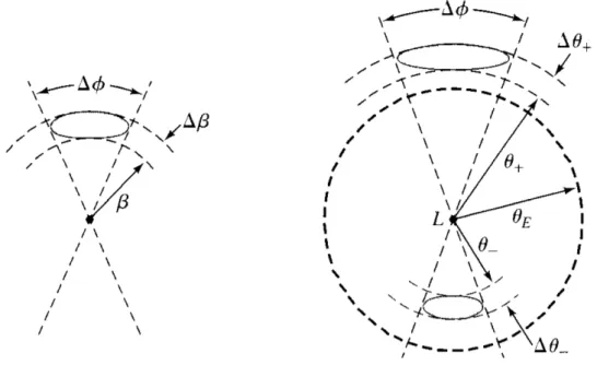
Figure 2.3: Image of galaxy if lens (located at L) was not present (left). The respective

images (atθ±) during the presence of a lens (right). The source is located at an angle

β from the observer-lens axis with angular dimensions of ∆φand ∆θ±. Note that the azimuthal width (∆φ) of the image, whether located atθ±, is always conserved. Image

from Hartle[2].

dΩ = Z Z

S

sinβdφdβ≈βdφdβ (2.11)

Using this we can define the magnification of the event to be the ratio of non-lens to lensed flux – this yields a proportionality between solid angles,

I± I∗

= ∆Ω± ∆Ω∗

(2.12)

where I∗ and ∆Ω∗ are the non-lensed intensity and solid angle, respectively. From

Equation 2.11, this can be defined as

∆Ω±

∆Ω∗

=|θ±∆θ±∆φ

β∆β∆φ |. (2.13)

By introducing the minimum angular impact parameteru to be

u= β

θE

, (2.14)

(16)

u=y−1

y, (2.15)

where y≡ _θθ

E, which, when solved for y, yields a quadratic of the form

y2−uy−1

y = 0. (2.16)

The solution to this equation is

y±u±

p

(u2_{+ 4)}

2 . (2.17)

Since the surface brightness of the source is conserved for this model, the ratio of solid angles defines the magnification, such that

A±= y±

u dy±

du , (2.18)

where the total magnification is given by

Atot =A−+A+. (2.19)

The solution to A±is

A±= 1 4 (u2±p (u2+ 4)2) up(u2_{+ 4)} , (2.20)

and thus Atot can be expressed as

Atot= 1 4 1 u√u2_{+ 4} 2u2+ 2(pu2_{+ 4)}2 . (2.21)

The microlensing magnification as a function of the impact parameter uis then

A(u) = u

2_{+ 2}

2√u2_{+ 4}. (2.22)

Thus a PSPL event can be described by three parameters, the timescale (tE), the

(17)

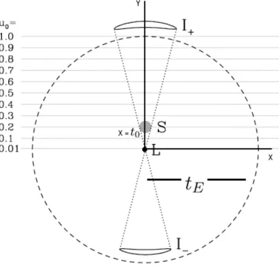
Figure 2.4: The geometry of a microlensing event as viewed from the perspective of the observer, source pictured at x=t0. Setting the lens (L) at the origin, and with a

fixed u0, u(t) can be be described as Equation 2.23. The total time it takes to cross

the angular Einstein radius is 2tE. Modified image, original from Gaudi[4].

of the event is the time it takes the source to cross the angular Einstein radius of the lens, we can define u(t) as the projected distance between the source and the lens, in terms of tE. By setting up a coordinate system with the lens mass at the center, any

position is given by the euclidean distance to the origin, with u0 being the analog of

y (as at x=0, y = u0; see Figure 2.4), and x = t−_tt0

E . This dimensionless parameter is

therefore u(t) = s u2 0+ t−t0 tE 2 . (2.23)

Thus one can define a microlensing event with the three functions of time[5]. The magnification factor A(t) describes the area of the image over the area of the source, with the second parameter being the overall flux F(t), which for our purposes is the apparent magnitude of the entire system in whatever photometric band the data is collected,

A(t) = u(t)

2_{+ 2}

(18)

Figure 2.5: Blending occurs when neighboring stars overlap in the CCD frame[6].

Only the light from one star exhibits microlensing behavior, making it important to subtract the additional blend flux to model the event correctly.

F(t) =A(t)fs, (2.25)

where fs is the source flux, also in apparent magnitude. The third function used is

distance between the source and the lens, u(t) as defined by Equation 2.23.

2.0.2 Blending

The PSPL model thus far assumes that the source flux in the CCD frame is isolated, such that the flux can be measured independently of any stellar neighbors. Unfortunately the most promising regions for microlensing detection, the Bulge and the Magallenic Clouds, are extremely crowded and the blending of light will yield deceptive results if unaccounted for. Even though stars can’t usually be resolved and analyzed as disks, the points of light from the source diffract at the telescope aperture, and the light from the star is spread out over a circle of pixels on the frame. The shape of this circle is determined by the point spread function (PSF) of the star[6], which will contain a certain full-width-half-maximum (FWHM) that is dependent on the telescope and weather conditions at the time. If two stars lie at close angular separation from our line of sight, their PSF will overlap and we say the event is blended (Figure 2.5).

To account for blending, Equation 2.25 is described as

(19)

Figure 2.6: Baseline magnitude as a function of the blending coefficient b. Data

compiled between 2003 and 2008 by OGLE-III[10]. For modeling events, we took 1≤

b≤10.

wherefb is the additional blend flux[7]. The overall observed flux is calculated as

Aobs(t) = fsA(t) +fb fs+fb . (2.27) Taking b= fb fs,Aobs(t) becomes Aobs(t) = A(t) +b 1 +b . (2.28)

In the event that the source causing the blending is not constant (e.g. variable star),

fb must be an appropriate function of time, like a sinusoid for a long period variable

star. Ultimately, accounting for blending requires guessing initial event parameters to derive an initial model for A(t), and inferring fb and fs by applying a χ2 test.

While constrainingbthrough the fitting process is the most common method for dealing with blending, it is also possible to actually resolve the stars contributing fb through

the use of space or large ground-based telescopes[8][9]. For our purposes of modeling microlensing, we only had to set a value for the blending coefficient b. From a previous analysis of microlensing events, we determined a blending coefficient between 1 and 10 was reasonable for modeling PSPL events (Figure 2.6).

(20)

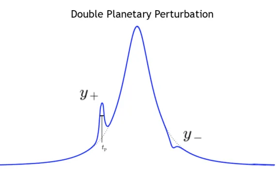
Figure 2.7: Example of a microlensing lightcurve with rare double planetary

pertur-bation. An increase in magnification occurs when a planet is near the Major image, with a decrease occuring when a planet gets near the Minor image. We can approximate

tp as the FWHM of the planetary signal. Modified image, original by J. Yee[6].

While in reality a lens is not a point source, this simple model serves to illuminate the basic fundamentals behind the microlensing theory, and was sufficient for our modeling of microlensing events, as described in Section 3.

2.0.3 Planetary Perturbations

Gaudi & Gould[11] demonstrated how the mass of a planet could be detected when perturbation occurs. Any planet that orbits the lensing star is detectable (to first order) only if it is located at either y± (Equation 2.17), denoted as θ± in Figure 2.4. If the planet is located in the Minor image (y−), the perturbation tends to destroy it, resulting

in a decrease in magnification[6]. On the other hand, if the planet is located in the Major image (y+), it will increase the magnification (Figure 2.7).

Another utility of our PSPL model is that it allows us to estimate the mass ratio between the lens star and a planetary companion by using the relation

θp =

m_p

M

1₂

θE, (2.29)

where θE is still the Einstein ring of the lensing star, θp is the planetary Einstein ring,

(21)

ratio of Einstein rings should be proportional to the timescales of both the event and perturbation, thus also proportional to the square root of the mass ratio,

θp θE = tp tE = m_p M 1₂ . (2.30)

Therefore, by measuring the mass of a star (through luminosity-temperature relation and/or spectral data), we can measure the mass of a planetary companion as

mp = tp tE 2 M. (2.31)

As microlensing is sensitive to any planetary mass, it remains the most promising tool to-date for detecting small, rocky worlds within the habitable zone of their host star.

2.0.4 Optical Depth

The microlensing optical depth is defined to be the probability of any given star being lensed at any one moment, assuming an amplification (Equation 2.24) of at least A ≈

1.34, given by requiring any event to be within one Einstein radius. Anything further out may be undetectable, as A trends towards 1 as the angular separation goes to infinity. Working off this consideration, the optical depth can be expressed as the ratio of a given solid angle of sky (dΩ) being lensed by the Einstein rings of all sources within that area. Therefore, the optical depth (τ) is

τ = 1

dΩ Z DS

0

n(DL)πθE2dV (2.32)

where n(DL) is the number density of lenses at a distance DL, and DS is the distance

to the source. From spherical trigonometry, dV =dΩD2_LdDL. From Equation 2.7, sub

inθE: τ = 4π Z DS 0 n(DL) GML c2 DLS DLDS D_L2dDL. (2.33)

The stellar number density up to a distance DL can expressed as

n(DL) =

ρ(DL)

ML

, (2.34)

(22)

τ = 4πG c2 Z DS 0 ρ(DL) DLSDL DS dDL. (2.35)

The integral can be solved using a substitution of variables, with x≡ DL

DS and dx = dDL DS , τ = 4πG c2 Z 1 0 ρ(x)DLSDSdx. (2.36) Since DLS =DS−DL, τ = 4πG c2 Z 1 0 ρ(x)xD2_S(1−x)dx. (2.37)

Taking the galactic density to be constant,ρ(x)⇒ρ0, the integral is simple to solve as

τ = 2 3

πGD2_Sρo

c2 . (2.38)

This can written in terms of the volume of a sphere with radiusDS, which when combined

with constantρ0serves as an approximation for the mass contained within this distance,

τ = 4 3πD 3 SρoG 2c2_D S ≈GM(DS) 2c2_D S . (2.39)

With the numerator now containing an expression for the total mass within a sphere of radiusDS, we can estimateτ through orbital mechanics by equating the expression for

centripetal acceleration and Newton’s law of universal gravitation,

mv2 DS

=GM(DS)m

D2_S , (2.40)

wheremcan be taken to be the mass of a satellite orbiting at distanceDS, which cancels

out after some algebra to get:

v2=GM(DS) DS

. (2.41)

This allows us to estimateτ by taking vto be the orbital speed of stars within distance

DS, and plugging back to Equation 2.39,τ can be approximated as

τ ≈ v

2

(23)

Figure 2.8: Rotation speed versus galactocentric radius for stars within the Milky

Way[12].

Figure 2.8 shows the rotational speed for stars as a function of radial distance from the center of the galaxy. Using a velocity of v ≈ 220 km/sec, the optical depth can finally be solved as τ ≈ (220000 m s) 2 2(3×108m s)2 ≈2.68×10−7. (2.43)

This turns out to be a decent approximation, with several microlensing surveys calcu-lating the optical depth toward the Galactic Bulge as τ = (3.3±1.2)×10−6 (OGLE team[13]) and τ = (3.9±1.8

1.2)×10−6 (MACHO team[14]). While this is an order of

mag-nitude larger than the approximatedτ ≈10−7, this is not too surprising, as the Galactic Bulge is a high density stellar field, where the probability of stellar alignment is higher. For a wide-field survey like the recently commissioned ZTF[15] in which billions of stars will be observed in the Bulge, one can expect hundreds of microlensing events within the survey footprint. Even for a survey as irregularly sampled as PTF, an extrapola-tion from previous all-sky rate estimates yielded an estimate of 1-10 detectable events within the survey[16]. We present now the development of the algorithm, and how it was applied to detect additional microlensing candidates in PTF.

(24)

Classification via Machine

Learning

The utility of microlensing comes in many different forms, from its ability to detect exoplanets[17], to the opportunity it presents to study isolated compact remnants such as black holes and neutron stars[18] and even study stellar properties[19]. With such a small optical depth, it is imperative to monitor hundreds of millions of stars in the search for these rare transient events. Two microlensing teams, OGLE1 and MOA,2 have contributed significantly in this field by conducting wide-field surveys, cataloging several thousand microlensing events each year [20][21].

As CCD technology continues to improve and the next generation of photometric wide-field surveys launch, it’s becoming increasingly necessary to develop techniques to distin-guish between variable stars and microlensing signals. As a rare transient phenomena, it’s important to detect these signals as early as possible so as to ensure time-domain data can be continuously collected and a complete lightcurve can be constructed. The Early Warning System (EWS) applied by the OGLE team flags sources if there’s an increase in flux past a certain threshold, for a pre-defined number of consecutive times. Plausible microlensing events are forwarded for visual inspection if the source was non-variable during the reference season(s), but as such requires every event to have a well-established baseline magnitude set from previous reference images[22]. KMTNet, another microlens-ing group operatmicrolens-ing three 1.6m telescopes with 4 deg2 cameras, relies on an algorithm that requires fitting the lightcurves to a dense grid of point-lens models[23], passing along stars that meet aχ2 threshold as plausible candidates for visual inspection. While these methods have been successfully applied to detect microlensing, they both can yield

1_{http://ogle.astrouw.edu.pl/} 2

http://www.phys.canterbury.ac.nz/moa/

(25)

Classification via Machine Learning 17

false-alerts that are often passed along for visual verification. In the case of planetary deviations, it is important to classify and monitor the source as early as possible as the event can be as short-lived as a few hours, making it of utmost importance that any human operator tasked with visually verifying alerts is not swamped with thousands of false-alerts each night.

The task of quick, automated classification has been tackled successfully over the past several decades through the use of machine learning. In particular, the Random Forest (RF) algorithm[24] has been applied with great success for variable star classification[10], as well as for classifying supernova and microlensing events[25][26]. The advantage of the RF algorithm is its simplistic application as well as the flexibility that allows it to be easily incorporated across multiple surveys, requiring only time-series photometric data to function. This research project aims at optimizing an RF algorithm to differ-entiate between microlensing lightcurves and that of other stellar classes of variables and transients. In this work, we used a subset of data from the intermediate Palomar Transient Factory (iPTF) described in section 3 to both develop the algorithm and test performance. While ≈ 1-10 microlensing events are to be expected in the iPTF foot-print, none have been detected and confirmed to date, mostly due to irregularities in the cadence that resulted in gaps in photometric data. A statistical approach was applied by Adrian Price-Whelan[16], in which he filtered for microlensing candidates in PTF by applying thresholds to variability indices calculated from the photometry, reporting three plausible microlensing events from a subset of≈2000 candidates. While different works implement different classification methods, a side-by-side comparison of ten dif-ferent classifiers in two difdif-ferent datasets (OGLE and Hipparcos)[10] found the Random Forest to have the lowest error rate; coupled with its swift performance the Random Forest is a strong algorithm for automatic classification and for this reason we sought to apply its utility for our research.

3.0.1 Random Forest Algorithm

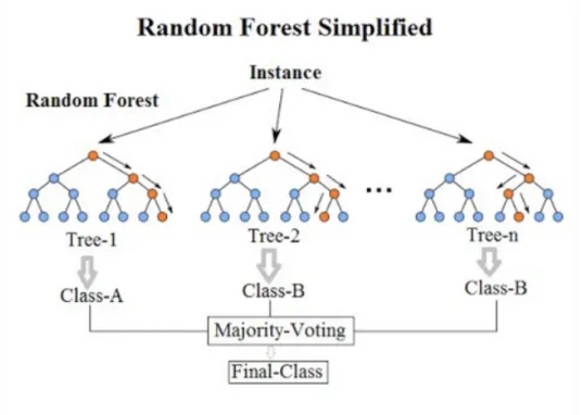
The Random Forest is an ensemble machine learning method that trains numerous decision tree classifiers and takes the mode of the classification results as the output, in effect combining a multitude of “weak” learners (individual decision trees) to create one “strong” learner (the ensemble).

Decision tree learning is used to map a set of input features to output classes by means of a series of selection rules determined during the training process. In this instance, it represents the mapping of statistical metrics to source class. A single tree in the ensemble is trained by generating a set of selection rules based upon whichever statistic

(26)

and given threshold outputs the maximum information gain (as is the case when features are continuous). Of course, given a set of features, the process of identifying the most robust metrics requires the use of some criterion, in which a value relating to information gain is calculated per each feature, and once sorted, the attributes that yield the most information gain (as determined by the criterion value) are placed near the root of the tree. The criterion applied here is the default metric in sklearn[27], the Gini-index, also known as ‘mean decrease impurity’.

This criterion is utilized to measure how often a feature (when chosen at random) would be incorrectly identified, such that a statistical features with a low Gini-index would be preferred, and the selection rules used to train the individual trees are based upon whichever features yield the lower index. The Gini-index is measured as[28]

G= 1−X

j

p2_j (3.1)

wherepjis the probability of class j. Using this index to measure impurity, the generation

of selection rules occurs recursively until a given three-depth (if pre-assigned) is reached, or all objects in the training set (within a given area of a tree) are of the same class. A single decision tree is considered to be over-fitted if the tree is ‘deep’ and contains too many node splits, hence too specific and thus has a high variance. On the contrary, a tree is consider to have low variance and be under-fitted if it’s ‘shallow’. Since an individual tree is not a good predictor on its own, we applied the use of the Random Forest, an ensemble method developed by Breiman[24], which mitigates the issue of poorly fitted decision trees by allowing groups of them to train deeply on a subset of features, as well as a subset of input data. The randomness in the algorithm is thus a result of a random combination of features being used to deeply train the trees each time.

To reiterate, the Random Forest grows an ensemble of decision trees by sampling subsets of the training data repeatedly (with replacement at each iteration), while also only selectingn number of features each time, such that

n << N, (3.2)

where n is a random subset of the N total features. Each individual tree is grown as deep as possible, until all the objects in the end branches yield a single class. Once trained, the Random Forest will classify new objects by inputting the features into the ensemble of decision trees, and after each tree outputs a single prediction, the mode of the class selections is outputted as the predicted class.

(27)

Figure 3.1: Public domain schematic of the random forest as it “votes” to determine

an output class by running features down individual decision trees. Each tree is trained on separate subsets of features and data. Diagram included in the sklearn package

documentation.

The hyperparameters available for tuning in the sklearn package were left untouched, as the defaults for the Random Forest were deemed appropriate for our classification task. We tuned only the number of trees used to train the forest. While more trees will yield more accurate results, a balance between performance and run-time must be optimized. We found the algorithm performance to plateau after 200+ trees were used for training, with negligible improvement with up to 1000 trees. Since less than 200 trees could at times yield a 1-2 percent difference (as per the random nature), we decided to train the algorithm with 300 trees. Next we discuss the data that was used to train the Random Forest.

3.0.2 Training Set

Random Forests effectively memorize the training data, and as such a RF classifier is only as accurate as its training set. The most important class in our bag is our target source – microlensing. Given our access to iPTF data (which includes all of PTF), we decided to train our algorithm using iPTF lightcurves. As no microlensing lightcurves (to date) have been identified in this dataset, we had to simulate how an event could have appeared in the irregularly sampled footprint.

(28)

Figure 3.2: log10(RMS) as a function of median fluxes for a subset of the PTF data

made available by Price-Whelan([16]). The quadratic relation is typical for wide-field surveys. Lightcurves that were below the fit and had ≥ 45 photometric points were

taken to have no variability and were used for the microlensing simulation.

We simulated microlensing as it would appear in the iPTF lightcurves by injecting PSPL parameters into constant lightcurves extracted from various iPTF fields. From here we will refer to ‘constant’ lightcurves as any lightcurve that shows no sign of variability. This particular dataset was made publicly available by Adrian M. Price-Whelan ([16]). From the approximately 10000 ligthcurves Price-Whelan released, 1646 constant lightcurves were extracted. These were selected by fitting a curve to thelog10(RMS) as a function of

median magnitude for the released data. Lightcurves that had≥45 photometric points and fell below a third degree spline fit were categorized as having no variability (Figure 3.2).

By injecting the PSPL parameters derived in Section 2 into real constant lightcurves, we manage to mimic the cadence of the survey footprint. To construct Aobs(t), we

referred to an analysis of microlensing events using six years of OGLE-III microlensing observations compiled by Tsapras[3]. From this study, we decided on the following values for our PSPL parameters:

1. The time of maximum amplificationto is selected randomly.

2. The angular impact parameter uo is chosen from a uniform random distribution

between 0 and 1.0 (Figure 3.3).

3. The Einstein crossing time tE (Figure 3.3). is chosen from a normal distribution

with a mean of 30 days and a standard deviation of 10 days.

(29)

Figure 3.3: Left: distribution of the minimum impact parameter, u0. The darker

histogram corresponds to microlensing events that have a blend fraction b≤0.1. The lighter histogram was generated using all events. Right: distribution of the event

timescaletE. Data from OGLE-III[3].

Given the randomness in the microlensing simulations, we had to include additional simulation thresholds to ensure a proper training set, as most events tend to be of low magnification and thus undetectable by iPTF. Since feasibly detectable microlensing signals are generated at random, we imposed the following additional parameters to guarantee we simulated only detectable signals.

1. The simulated magnification between to±tE must be greater than the non

simu-lated magnitude by at least 0.05.

2. At least one third of photometric measurements must be magnified at least 3σ, such that one third of values in [A] are greater than 3, where [A] is the following list: [A] = _m0 i−mi σi , (3.3)

where i denotes all indices within t0 ±tE. m is the non-simulated photometric

points of the lightcurve, m0 is the simulated photometric points, and σ is the photometric error.

3. Lastly, the peak magnificationAmax (quantified as _u1_o) must be> f_fs_b.

These magnification thresholds were used to ensure that proper signal was input into our simulated microlensing events. In total, we simulated 400 microlensing events for training and testing purposes. While there are many sources that mimic microlensing behavior (like novae), we decided to train the Random Forest primarily on two classes of variables that can yield a high number of false alerts: Cataclysmic Variables (CV) and

(30)

Figure 3.4: Sample lightcurve of a cataclysmic variable[29]. The microlensing-like

increase in magnitude can yield false-alerts when data is incomplete.

Figure 3.5: Sample lightcurve of a RR Lyrae variable[30]. The microlensing-like

increase in magnitude can yield false-alerts when data is incomplete

RR Lyrae Variables. From the available iPTF data, we extracted lightcurves for 216 CV, 318 RR Lyrae, and 316 sources labeled as ‘other’. These sources were carefully classified through the efforts of the PTF collaboration3. While our training bag for constants was significantly larger than all our other classes, we decided to only use 500 for training and testing the algorithm, as overfitting can occur when there’s a substantial disparity between individual training bags. All the data selected for training had at least 45 measurements, and were inspected to ensure that they were representative of the source class.

From the 500 constant stars, 200 were lightcurves that included only the first 2-30 points (selected at random) to avoid confusion when only few measurements are available. The ‘other’ class contained the sources displayed in Table 3.1.

3

(31)

Classification via Machine Learning 23 subclass subclass AGN 61 G/K Star 11 AMCVn 14 LPV 61 Cepheid 21 Mira 22 δScuti 12 QSO 34 dME 12 R CrB 10 EcBinary 35 YSO 23

Table 3.1: Other Classes of Variables/Transients Included

3.0.3 Algorithm Performance

While the achromatic nature of microlensing can help in eliminating false-alerts, we make no attempt to implement a use for multi-band photometry, instead, we focus on classification only using single-band data, as it generalizes the use of the algorithm and allows for ease in utilization across different databases. Each lightcurve in our training set is described by a set of statistical features, which are input as a vector into the classifier. As outlined in the previous subsection, we utilized the Random Forest algorithm available in the open source Python package, sklearn. Given both its simplicity and the availability of documentation as a result of its widespread implementation in numerous disciplines, this machine learning implementation is a powerful tool. We find the default Gini-index impurity method applied by sklearn to assess feature importance to be accurate and consistent with past research. The most important metric identified was StetsonJ, denoted as J, a variability index first suggested by Stetson [31] and recently applied as a useful metric for identifying microlensing candidates in PTF[16]. A more robust version of the Welsch/Stetson index, J is quantified as

J = n−1 X i=1 sign(δiδi+1) p |δiδi+1 |, (3.4)

where the sign function corresponds to the sign of the argument (+1 for positive, and -1 for negative) and δi is

δi= r n n−1 xi−x¯ ei , (3.5)

whereei is the photometric error of each individual data point. This product of the

nor-malized residuals is used to relate two consecutive observations (the ‘i’th pair), with δ

serving as a “relative error”. The magnitude ofδis the residual of a given measurement from the mean scaled by a standard error (the term withei) . The original

(32)

for single-band use, it accounts for the fact that the observation itself is being used to define the mean hence the residual from the sample mean is (on average) smaller than it should be, by considering a bias factor that’s dependent on the total number of n

observations available to compute the mean[31]. As constructed, this index will trend to 0 for variable sources and gets large as the difference between the successive data points increases.

In addition to J, the sklearn module also identified the von Neumann ratio η as an important metric, defined in 1941 by John von Neumann[32] as a measure of dependence within a set of observations,x1, ..., xn. This statistic serves as the mean square successive

difference divided by the sample variance,

η = Pn

i=1(xi−1−xi)2/(n−1)

σ2 . (3.6)

Whenηis small, it is an indication of a strong positive correlation between the successive photometric data points, serving as another useful metric for identifying variables. By starting with over 20 features, we analyzed algorithm performance by splitting our data into two, using one set for training the algorithm and one set for testing. By discarding the lowest performing feature at each iteration while keeping the classification accuracy as high as possible, we were able to select the 13 most important features as determined by the random forest, all displayed in Table 3.2 at the end of this chapter (for information on all the features, see the program documentation[33]). Discarding poor-performing features is important as it helps prevent overfitting when training the algorithm, and also decreases the time it takes the classifier to run. Figure 3.6 displays the feature importance, highlighting the top three features.

To visualize algorithm performance, we constructed both a receiving operating charac-teristic (ROC) curve (Figure 3.7) and a confusion matrix (Figure 3.8). A ROC curve allows for a visualization of the trade-off between the true positive rate (TPR), and the false positive rate (FPR), both as a function of the classification threshold applied. When the RF classifies an object, it outputs a probability prediction ranging from zero to one, allowing for a threshold to be applied such that the classifier won’t flag a source unless the probability prediction exceeds this value. Varying this parameter allows us to visualize algorithm performance. The TPR is defined as

TPR = TP

TP+FN, (3.7)

which, for the case of microlensing, serves as the ratio between the correctly classified microlensing events (True Positive) and the total number of events in the bag (True

(33)

Figure 3.6: Feature importance as determined by the RF. The algorithm makes use of 13 lightcurve statistics for classification, including robust and devised metrics, as well as variability indices previously applied by Price-Whelan[16] and Richards[10].

Figure 3.7: Confusion Matrix displaying algorithm performance. A perfect classifier would yield a value of 1.0 on the diagonals, signifying correct classification 100% of the

(34)

Figure 3.8: ROC curve for our dataset. The lower value of the AUC for the ‘other’ class is consistent with the higher rate of misclassification as displayed in the confusion

matrix.

Positive + False Negative). Likewise, the FPR is the ratio of incorrectly classified microlensing to the total number of non-microlensing lightcurves in the dataset,

FPR = FP

FP+TN. (3.8)

An ideal classifier would maximize the TPR while simultaneously minimizing the FPR. A useful metric that can be extracted from the ROC curve is the area under curve (AUC). When the AUC is one, the TPR is maximized and the FPR is minimized, indicating a perfect classifier. In the same regard, a classifier with an AUC of less than 0.5 would indicate a classifier that performs worse than random. We find the best performance occurs with the constant class, as expected given the lack of signal in these lightcurves. The second curve with the highest AUC is that of microlensing, with the lowest performing class (‘other’) yielding an AUC of 0.94.

The confusion matrix was constructed by splitting the entire training data into two sets, split evenly across each class. We trained the Random Forest with half the data, and con-structed a confusion matrix from the remaining test data. As the data is split randomly, this serves as a simple, yet effective method for visualizing classification accuracy. Over-all the algorithm performed well, correctly classifying 95% of true microlensing, with the lowest performance being an accuracy of 68% with the ‘other’ class. We find that for our classes of variables CV and Lyrae, only about 5% are predicted as microlensing, with the most false-alerts (10%) occuring with the ‘other’ class. Given that 12 different

(35)

stellar subclasses were included in this bag, at varying quantities, it’s not surprising that the algorithm is especially confused with this class. Overall though, the values in the confusion matrix are consistent with the ROC Curve, in which the ‘other’ class yielded the lowest performance, followed by CV. Overall though, the algorithm performs better than random, and in regards to microlensing classification in particular, it’s extremely accurate despite the 5-10% of false alerts that occur from our other classes of variables.

(36)

Metric Definition

Shannon Entropy Shannon entropy[34] is used as a metric to quantify the amount of information carried by a signal. The procedure employed here follows that outlined by (D. Mislis et al. 2015)[26].

Kurtosis Kurtosis function returns the calculated kur-tosis of the lightcurve. It’s a measure of the peakedness (or flatness) of the lightcurve rela-tive to a normal distribution.

Skewness Skewness measures the asymmetry of a

lightcurve, with a positive skewness indicating a skew to the right, and a negative skewness indicating a skew to the left.

vonNeumann Ratio The ratio η was defined in 1941 by John von Neumann[32] and serves as the mean square successive difference divided by the sample variance. When this ratio is small, it is an indi-cation of a strong positive correlation between the successive photometric data points.

stetsonJ This variability index was first suggested by Peter B. Stetson[31] and serves as a measure of the correlation between the data points, tend-ing to 0 for variable stars and getttend-ing large as the difference between the successive data points increases.

stetsonK This variability index first suggested by Stetson Stetson[31] serves as an alternative measure for the kurtosis of a distribution.

Amplitude To account for outliers prior to computing, an array of the absolute value of the magnitude minus weighted mean is created. From this ar-ray, a 5% threshold is applied such that top 5% of points are omitted as outliers and the am-plitude is left to be defined as the maximum magnitude minus the minimum magnitude of the remaining points.

Median Buffer Range This function returns the ratio of points that are between plus or minus 10% of the ampli-tude value in respect to the mean.

Standard Deviation over Mean A measure of the ratio between standard de-viation and mean magnitude, weighted by the errors.

Below 1 This function measures the ratio of data points that are below 1 standard deviation from the mean magnitude.

Median Absolute Deviation A measure of the mean average distance be-tween each magnitude value and the mean magnitude.

RMS A measure of the root mean square deviation, weighted by the errors.

Median Distance This function calculates the median euclidean distance between each photometric measure-ment, found to be a helpful metric for detecting the overlapped lightcurves.

(37)

Chapter 4

Phase Two: Fitting with pyLIMA

We find that despite a few misclassified microlensing, the algorithm performed well in distinguishing between true microlensing signals and other types of transients and variables. Nonetheless, given the need to monitor millions of stars, even 1% of sources being flagged can yield a huge number of misclassifications, too many to visually inspect. To further filter out variables, we applied the use of the open source microlensing fitting algorithm pyLIMA[35]. This program is designed to model microlensing events as Point-Source or Finite-Point-Source Point Lens. For our purposes we utilized pyLIMA to fit a PSPL model to all candidates flagged by the Random Forest, allowing us to further filter out poor candidates by restricting the PSPL parameter space.

4.0.1 Levenberg-Marquardt

The first fitting method that’s tried is based on the Levenberg-Marquardt algorithm[36][37], which in pyLIMA is based on the scipy.optimize.leastsq Python routine[38]. This is a commonly applied mathematical procedure to fit the best fit line (or any multivari-ate equation) to a set of data points. This is an iterative technique that identifies a local minimum of a multivariate function that’s expressed as the sum of squares of non-linear functions, fi(x). For fitting a function φ(t;x) to empirical, time-domain data

{(ti, yi), i = 0, ..., n−1}, it is common practice to use a quadratic, scalar loss function

of the form[39]

fi(x) =wi(yi−φ(t;x)), (4.1)

wherewi are weights applied to each observation, which for our case can be taken to be

wi= 1. Thus, this method works by minimizing the sum of the squares of the offsets of

(38)

the data points from the regression function (referred to as residuals), and givenndata points (xi, yi), we can model the function φ(t;~x) to the data, and as such identify the

best fit parameters ˆx, which occurs when the sum of the residuals is minimized (when the sum of the residuals is 0, the data points fit perfectly within the model φ(t;~x)),

ˆ x= min n X i=1 [yi−φ(t;~x)]2. (4.2)

Thus, we can estimate the PSPL microlensing parameters by fitting for the observed flux,

φ(t;~x) =Aobs(t;~x), (4.3)

and making our time-domain flux measurements yi. The Levenberg-Marquardt

algo-rithm allows us to discard variables and/or faulty signals that may get misclassified by the RF by restricting the microlensing parameter space to reasonable observables. A lightcurve is flagged as true microlensing only if the fitted PSPL parameters meet the following conditions:

1. tE must be greater than one day.

2. u0 must be greater than 0 and less than 2.0.

3. There are at least two points within the timescale of the event.

4. Reduced χ2 of LM fit is less than three.

The least-squares minimization method utilizes the Jacobian matrix (Jij) for finding

the minima, and can fail ifJij is non-differentiable (as can often happen when there are

outliers in data). As pyLIMA outputs an error value for each best fit parameter, we can check whether the LM method failed by checking the error volume oft0, tE, andu0,

defined as

vol=t0tEu0, (4.4)

in which any given value forbeing 0 (which happens when the parameter is undefined) will yield

(39)

Phase Two: Fitting with pyLIMA 31

indicating a failed LM fit. When this occurs, we apply a more time-consuming, but robust method, the Differential Evolution algorithm.

4.0.2 Differential Evolution

The Differential Evolution (DE) algorithm developed by Storn and Price[40] is a heuristic approach that makes no assumption about the solutions, and can thus explore a larger candidate space, at the expense of computation time. In addition, due to the heuristic nature of this method, the true solution may not actually be explored if the search radius is not large enough, and thus the true solutions will not be found.

Unlike the LM method, differential evolution does not depend on the gradient (and hence

Jij), and as such does not require the optimization problem to be differentiable. This

is because DE optimizes the problem at hand by generating a population of candidate solution vectors, creating new candidate vectors by combining (“mutating”) existing candidates together and keeping only candidate solutions that yield the best score for the problem at hand. The formula for creating new candidates is the default used by scipy, the ‘best1bin’ strategy, which is initialized by randomly selecting two population members and taking their difference (also multiplied by a random value in the range [0,2], referred to as the mutation factor or differential weight) to create the best member in this bin (for more information on the mutation process, see the scipy documentation[38]), reiterating until the population converges. The mutation process requires that solution vectors be continuously updated by either swapping candidate vector components or through some arithmetic combination of different trial and candidate vectors, continuing until an optimal solution is found or the population size limit is reached. The scipy module allows for the simple tuning of the hyperparameters, allowing the user to increase the odds of finding a global minimum by not only increasing the allowable population size, but also increasing the mutation factor which is used to mutate the best members. Increasing the mutation factor as well as the allowable population size allows us to expand our search radius, but slows down the process of convergence. We make no attempt to tune these hyperparameters in this research, and instead rely on the default values selected by pyLIMA. If no solution is found using DE, we discard the candidate and pass it through the pipeline as some ‘other’ stellar class.

To reiterate, DE is only applied when LM fails (as LM is more time-efficient), with the outputted DE parameters still subjected to the same conditions as before. Only lightcurves that are both detected by the RF and fall within our parameter space are forwarded along for visual inspection. We find that about 1% of input lightcurves are flagged by the RF as microlensing, with our pyLIMA fitting process eliminating an

(40)

additional 99%+ of those initially selected, leaving us to inspect approximately 800 lightcurves per million.

(41)

Chapter 5

Results

5.0.1 iPTF

The iPTF survey originally began as PTF in 2009, making use of the 7.26-square degree CFHT12k mosaic on the Palomar Samuel Oschin Schmidt 1.2-meter Telescope. The survey transformed into iPTF in 2012, still using the same telescope but with improved instruments, as well as with better performing data-reduction software. While the sur-vey is primarily operated in the R-band, additional observations in the g-band were occasionally performed. Utilizing an exposure time per frame of 60 seconds, the survey yields a 5-sigma limiting magnitude of 21 for the R-band, and 20.5 for the g-band. The survey was significantly upgraded once again, with the transition from iPTF to ZTF (Zwicky Transient Facility) finalizing earlier this year, 2018.

The first statistical search for microlensing events in the PTF database was performed by Price-Whelan, in which he discovered three plausible candidates[16]. One of the three events was later discarded when iPTF collected more data, the two remaining candidates are displayed in Figure 5.1. As PTF was irregularly sampled, the events detected by Price-Whelan are inconclusive, as no other survey to date has reported on these candidates and the available PTF data is not enough to make an assertive determination.

Price-Whelan’s method for querying PTF data and selecting plausible microlensing is not a real-time procedure, as is the case for our RF classifier. To visualize how these events would have been assessed by our RF algorithm had it been operating in real-time, we drip-fed these events into the classifier one point at a real-time, recording the RF prediction at each data point. This drip-feeding procedure is displayed in Figures 5.2 and 5.3, demonstrating the predictive power of the machine learning phase of our algorithm. Note that for both events, our Random Forest classifier detected the signal

(42)

Figure 5.1: Two of the three microlensing candidates identified and fitted with a

PSPL model by Price-Whelan[16].

Figure 5.2: Top: Microlensing candidate first detected by Price-Whelan. Bottom:

Drip-feeding the lightcurve into our classifier reveals at which epoch the classifier would have detected the event.

almost immediately (microlensing prediction occurs when the ML probability prediction is higher than all the others)

While iPTF data from the Galactic Bulge and Plane are currently unavailable due to re-processing efforts, I was allotted access to the rest of the iPTF database, and thus searched for microlensing in different areas of the survey footprint. During our search we encountered a peculiar problem as the RF flagged about 15% of inputted lightcurves as microlensing, which yielded way too many lightcurves to proccess. Upon closer examination we discovered a class of problematic lightcurves yielding false-alerts

(43)

Results 35

Figure 5.3: Top: Microlensing candidate first detected by Price-Whelan. Bottom:

Drip-feeding the lightcurve into our classifier reveals at which epoch the classifier would have detected the event.

Figure 5.4: Example of a type of lightcurve that was misclassified as microlensing.

The photometric points are stacked in a non-natural way as a result of a problem with the photometric pipeline.

that appeared to be a result of a faulty pipeline. Figure 5.4 shows such a lightcurve, which appears to be two individual lightcurves stacked on one another.

As a workaround to this problem we modified the training set for the algorithm to in-clude an additional “bad” class that we categorized as lightcurves with poor photometry (similar to that displayed in Figure 5.4), all extracted from the misclassified microlens-ing signals durmicrolens-ing our first run. In general, when devismicrolens-ing a trainmicrolens-ing bag for machine learning efforts, it’s best to keep the quantity of sources per class as even as possible so as to not bias the classifier toward any one class. We trained the algorithm with 300 of these ‘bad’ lightcurves to roughly match the size of our other classes. Unfortunately

(44)

Figure 5.5: Confusion Matrix displaying algorithm performance. We find that we are

able to filter out these ‘bad’ lightcurves virtually all the time when we increase the size of our training classes.

including this sub-sample resulted in a less accurate classifier, a problem we circumnav-igated by increasing the size of our ‘bad’ class to 700. For class-size consistency, we included CV and Lyrae into our ‘other’ class, and increased the number of microlensing and constant stars used for training to 1200 and 1600, respectively. This new training set yielded a better performance when distinguishing between microlensing and these ‘bad’ lightcurves, while sacrificing performance with the ’other’ class. It was a trade-off between accuracy and more false-alerts, but until the iPTF database is completely re-processed and the photometric pipeline fixed, we found this to be the best method for filtering out these problematic lightcurves.

In addition to modifying the training set, we included an additional metric that we found to work well at detecting these ‘bad’ lightcurves, the median euclidean distance between the photometric points. It is particularly useful in that for these problematic lightcurves this metric tended to be significantly higher. We defined this new metric as

MedDistance = median{p(ti+1−ti)2+ (mi+1−mi)2 }, (5.1)

wheret is the time, andm is the magnitude.

In conjunction with the new classifying algorithm we applied the following additional filters to further eliminate problematic lightcurves:

(45)

Results 37

1. Only ingested lightcurves with ≥45 photometric points.

2. At least 95% of all points in the lightcurve must not be flagged as bad points.

3. The baseline magnitude must be>14 and <20.

4. Only microlensing detections with at least a 60% confidence were saved.

Using these filters we found that we were detecting ∼1% of all ingested lightcurves as microlensing. While still more than what we expected, it was a significant improvement from the initial 15%. Since iPTF data is not being inputted in real-time, we worked off the assumption that for this particular search, any microlensing event must have occurred already. This allows us to further filter out lightcurves by requiring a certain number of measurements in the entire signal (t0±tE). We chose an arbitrary value of

at least 7 measurements within the timescale, and furthermore clustered our data using the scipy implementation for hierarchical clustering analysis[38]. Using this clustering algorithm, we loosely grouped our time-domain data, such that data gaps of more than 100 days were considered to be separate clusters. By requiring the signal to be within one cluster, we eliminated scenarios in which pyLIMA would falsely fit a largetE event

across several time clusters, where no signal was present in the first place. While mi-crolensing events with long timescales are certainly a possibility, the averagetE is about

30 days as shown in Figure 3.3, and thus we decided that additional filtering through hierarchal clustering was worth implementing. In summary, our conditions for searching for microlensing events in iPTF were:

1. The timescale tE of the event must be≥ 1 day.

2. The minimum impact parameter u0 must be ≤1.5.

3. The χ2 of the fit must be <1000.

4. There must be at least 7 points in the microlensing signal, with at least one measurement within ± 1

2tE.

5. The microlensing event must occur within one timescale cluster, clustered by a time threshold of 100 days.

Fitting every lightcurve detected by the Random Forest and applying these thresholds eliminates ∼ 90% of lightcurves as poor candidates. Coupled with the initial filters, this filtering method leaves ∼800 lightcurves per million to be visually inspected. For this preliminary test we have ingested 3.2 iPTF million lightcurves into the algorithm, at a rate of ∼7 lightcurves per second. We present the three microlensing candidates

(46)

Figure 5.6: Microlensing cadidate with equatorial J2000 RA and DEC in decimal degrees: (300.246157373, 22.962527584). A cross-match with SIMBAD reveals that the closest source to these coordinates is a star>100 arcseconds away from the epicenter.

Figure 5.7: Microlensing cadidate with equatorial J2000 RA and DEC in decimal

degrees: (298.333033149, 24.7609154852). A cross-match with SIMBAD reveals that the closest source to these coordinates is an infrared source 97 arcseconds away from

the epicenter.

(Figures 5.6-5.8) that we identified in the iPTF database. None of these have any nearby cross matches in SIMBAD, and remain uncategorized by the iPTF collaboration. Three plausible candidates for the 3 million lightcurves inspected is not too unreasonable given the optical depth, but without additional data these lightcurves remain inconclusive as none of these potential microlensing signals were measured in their entirety.

We plan to re-run our algorithm on iPTF as soon as the data for dense stellar fields (Bulge & Plane) is reprocessed and available.

(47)

Results 39

Figure 5.8: Microlensing cadidate with equatorial J2000 RA and DEC in decimal degrees: (296.9056637, 23.3270276814). A cross-match with SIMBAD reveals that the closest source to these coordinates is a star 64 arcseconds away from the epicenter.

5.0.2 ROME/REA Project

The ROME/REA Project is an international effort to detect small exoplanets beyond the snowline (where liquid water can exist) by detecting and monitoring microlensing events toward the Galactic Bulge1. Contribution data is gathered by several 1-meter robotic telescopes in the Southern Hemisphere, all operated by the Las Cumbres Observatory (LCO). Detected microlensing signals are then cross-matched and analyzed using time-domain data collected by other teams. In addition, the project aims at prioritizing microlensing signals with the highest probability of revealing a planetary perturbation – this is done by calculating the optimal frequency at which individual ongoing events need to be observed, thus prioritizing events that require high frequency sampling in an attempt to maximize the probability of detecting planetary signals.

As development for this microlensing detection algorithm was made possible due to the microlensing research group at LCO, I was allotted access to a sample of the data collected using the 1-meter Southern telescopes. This was not a blind test, as two events were known and identified previously. To assess algorithm performance in this survey, I inputted 96 thousand lightcurves (measured using the ‘i’ band), collected over several months by the 1-meter LCO telescope in Chile. From these 96 thousand sources, 1211 were flagged by the Random Forest, with 80 making it through the pyLIMA phase and forwarded for visual inspection. These numbers are consistent with our results using iPTF data. Of these 80, only two were true microlensing signals, with the rest being misclassified variables, some which required cross-checking with additional databases as lack of data made the signals appear like true microlensing.

1

(48)

Figure 5.9: Top: Microlensing event with equatorial J2000 RA and DEC in decimal

degrees: (268.33051201, -30.21089307). Bottom: Drip-feeding lightcurve reveals at which epoch this ROME/REA event would have been detected.

Figure 5.10: Microlensing event with equatorial J2000 RA and DEC in decimal

de-grees: (298.32281086, -30.18382827). Bottom: Drip-feeding lightcurve reveals at which epoch this ROME/REA event would have been detected.

(49)

Results 41

While hundreds of microlensing events have been detected through the ROME/REA collaboration, we were only allotted a subsample of data for testing the algorithm. While ultimately we seek to improve the classification process in an attempt to minimize false-alerts, we find that 2 true signals out of 80 candidates is a pretty good considering almost 100 thousand lightcurves were inserted for classification.

(50)

Conclusion

This detection algorithm is a licensed, open-source program that has been optimized for microlensing detection in any wide-field survey, with the microlensing training set easily modifiable to match the cadence of any given survey (instructions available in the documentation[33]). This algorithm is not designed to effectively detect any one particular class of variables, and as such should not be used to identify non-microlensing signals. For a discussion on the development of a variable star classifier, see (Richards et al. 2011)[10].

In addition to continuing our search in the iPTF database, we seek to also employ this algorithm to search for microlensing in the ZTF survey. All of our tests thus far have indicated high performance with promising early-detection capabilities, although we have yet to run the algorithm with real-time data. While iPTF, ZTF, and ROME are opportunities for microlensing search in the near future, the development of this program is currently funded with the hopes of employing it for early-detection in the Large Synoptic Survey Telescope (LSST)[41]. LSST is expected to begin science operations in 2022, covering ten square degrees of sky with a 3.2 billion pixel camera1. LSST will dominate time-domain astronomy as it releases terabytes of image data (up to 20 per night) that will be impossible to analyze entirely without the use of automated mining algorithms.

The range of science opportunities LSST will provide is immense, especially in the field of microlensing as LSST will provide time-domain data for billions of stars, with the potential of detecting thousands of events each year. There are ongoing efforts to include automated classification into the ANTARES system that LSST will use to forward along alerts (for a detailed description on the development of an LSST alert stream, see (Narayan et al. 2018)[42]). In collaboration with LSST collaborators, we

1_{https://www.lsst.org/lsst}

(51)

Conclusion 43

will be optimizing the algorithm for real-time microlensing detection in the LSST era. As LSST will provide multi-band photometry, we seek to take advantage of the achromatic nature of microlensing by integrating additional filtering modules into the classifier.

(52)

[1] D. Bennett. Detection of extrasolar planets by gravitational microlensing. In

Exoplanets, pages 47–88. Springer, 2008.

[2] J. Hartle. Gravity: an introduction to Einstein’s general relativity, volume 1. 2003.

[3] Y. Tsapras, M. Hundertmark, K. Horne, A. Udalski, C. Snodgrass, R. Street, D. Bramich, M. Dominik, V. Bozza, R. Jaimes, et al. The ogle-iii planet detection efficiency from six years of microlensing observations (2003–2008). Monthly

Notices of the Royal Astronomical Society, 457(2):1320–1331, 2016.

[4] B. Gaudi. Exoplanetary Microlensing. ArXiv e-prints, February 2010.

[5] B. Paczynski. Gravitational microlensing by the galactic halo. The Astrophysical Journal, 304:1–5, 1986.

[6] R. Street. Microlensing source. URL

http://microlensing-source.org/tutorial/.

[7] C. Han. Analytic relations between the observed gravitational microlensing parameters with and without the effect of blending. Monthly Notices of the Royal Astronomical Society, 309(2):373–378, 1999.

[8] J. Janczak, A Fukui, Subo Dong, LAG Monard, Szymon Koz lowski, A Gould, J. Beaulieu, Daniel Kubas, J. Marquette, T Sumi, et al. Sub-saturn planet moa-2008-blg-310lb: likely to be in the galactic bulge. The Astrophysical Journal, 711(2):731, 2010.

[9] D. Bennett, J. Anderson, I. Bond, A. Udalski, and A. Gould. Identification of the ogle-2003-blg-235/moa-2003-blg-53 planetary host star. The Astrophysical Journal Letters, 647(2):L171, 2006.

[10] J. Richards, D. Starr, N. Butler, J. Bloom, J. Brewer, A. Crellin-Quick, J. Higgins, R. Kennedy, and M. Rischard. On machine-learned classification of variable stars with sparse and noisy time-series data. The Astrophysical Journal, 733(1), May 2011. ISSN 0004-637X.