Implementation of Interpretive Structural Model and Topsis in
Manufacturing Industries for Supplier Selection
Rachit Kumar Verma
Department of Mechanical engineering, Madhav Institute of Technology and Science, Gwalior M.P-474005, India. [email protected]
Abstract:
The world is becoming international marketplace and the international environment is pushing industries to take practically everything into attention. In recent years supplier selection and order distribution as an important part of supply chain management are facing extraordinary challenges and difficulties. High customization and fast changing market stresses on modern supply chain management. Growing flexibility is needed to remain competitive and respond to quick changing market in this state supplier selection represents one of the most significant function to be done by the purchasing division. Supplier selection is the process by which industries classify, calculate, and deal with suppliers. In order to select the finest supplier it is necessary to make a compromise between these tangible and intangible criteria. The supplier selection method deploys a tremendous amount of a firm’s financial resources. In return, firms expect significant benefits from contracting with suppliers presenting high value. This research investigates and examines supplier selection criteria and the impact of supplier selection to the industry performance. Interpretive structural modeling (ISM) and technique of order preference by similarity to ideal solution (TOPSIS) methods are used by the researcher for selecting finest supplier. ISM help to find the important criteria used by the firm and topsis give the rank to the supplier. The results show that the planned method is capable of improving the shape of manufacturing systems and delivers pictured information for decision manufacturers.
Keywords: - Supply Chain Management, Supplier Selection, ISM, TOPSIS Method
INTRODUCTION: - A supply chain is a arrangement of societies, publics, events, information, and incomes
involved in moving a goods or facility from supplier to consumer. Supply chain activities renovate natural resources, raw materials, and components into complete merchandise that is transported to the end customer. Supply chain management (SCM) is the management of the movement of things. It contains the flow and storage of raw materials, work-in-process inventory, and completed goods from point of foundation to depletion. Interrelated systems, stations and knot constructions are involved in the running of products and facilities required by end customers in a supply chain. Supply chain management has been defined as the "design, planning, execution, control, and watching of supply chain events with the objective of creating net value, constructing a modest organization, leveraging universal logistics, matching supply with demand and measuring performance worldwide. The term "supply chain management" was first created by Keith Oliver in 1982. Nevertheless, the thought of a supply chain in management was of great reputation long before, in the early 20th century, especially with the making of the association line. A supplier is an external unit that supplies comparatively common, off the projection, or quality product or facilities. A supplier, in a supply chain is an originality that donates goods or services in a supply chain. A supply chain supplier productions inventory items and wholesales them to the next bond in the chain. Suppliers may or may not function as distributors of goods. They may be a function as manufacturers of product. If suppliers are also constructors, they may work as both to build a stock or build to order. Supplier is often a common term, used for suppliers of organization from retail sales to manufacturers to city organizations. Supplier mostly applies only to the industries that is rewarded for the goods, rather than to the new manufacturer or the industries performing the service. There are large no of suppliers in the global market for a same product, Quality, Price, etc. due to this reason a problem to select most efficient supplier for industries in created. To solve the selection of most efficient supplier out of no of supplier, researcher develops a method for selecting best supplier in two stages. First is to select most effective criteria in the supplier selection procedure by using Interpretive Structural Modeling. Second on the basis of these criteria’s develop a Technique for Order of Preference by Similarity to Ideal Solution (TOPSIS).
INTERPRETIVE STRUCTURAL MODELING: - Interpretive structural modeling is a computer assisted learning process was developed in 1973 by John N. Warfield at Battele Memorial Institute. Warfield proposed
understanding for the group’s almost great deal of analysis and communication takes place during an ISM session. The various steps involved in the ISM technique are as follows:
a) Identifying elements which are relevant to the problem or issues-this could be done by survey;
b) Establishing a contextual relationship between elements with respect to which pairs of elements would be examined;
c) Developing a structural self-interaction matrix (SSIM) of elements which indicates pair-wise relationship between elements of the system;
d) Developing a reachability matrix from the SSIM, and checking the matrix for transitivity – transitivity of the contextual relation is a basic assumption in ISM which states that if element A is related to B and B is related to C, then A is related to C;
e) Partitioning of the reachability matrix into different levels;
f) Based on the relationships given above in the reachability matrix, drawing a directed graph (digraph), and removing the transitive links;
g) Converting the resultant digraph into an ISM-based model by replacing element nodes with the statements; and
h) Reviewing the model to check for conceptual inconsistency and making the necessary modifications. After literature review and expert opinion of the survey response from organization following 20 criteria has been identified. These criteria’s are listed below.
1) Capacity 2) Communication system 3) Delivery 4) Employee education 5) Financial position 6) Flexibility 7) Geographical location 8) No. of employee 9) Attitude 10) Production facility 11) Price 12) Quality 13) Customer service 14) Reputation & position 15) Responsiveness 16) Reliability 17) Technology level 18) Warranties 19) R & D capability 20) Technical capability.
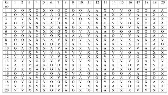
STRUCTURAL SELF-INTERACTION MATRIX (SSIM): - ISM methodology suggests the use of expert opinions based on management techniques such as brain storming, nominal group technique, etc. in developing the contextual relationship among the enablers. Group of experts, from industries and the academics were consulted in identifying the nature of contextual relationships among the barriers. For analyzing the barriers in developing SSIM, the following four symbols have been used to denote the direction of relationship between barriers (i and j):
V - Barrier i will help to achieve barrier j; A - Barrier j will help to achieve barrier i;
X - Barriers i and j will help to achieve each other; and O - Barriers i and j are unrelated.
Table-1 Structural Self-Interaction Matrix Cr. no 1 2 3 4 5 6 7 8 9 10 11 12 13 14 15 16 17 18 19 20 1 X O X O X O O O O O A A X V V O O O A A 2 O X A X A A O O A V A A A X X V A A X A 3 X V X V V V V V V O X X V A X A V O X X 4 O X A X X A O X A X A X O V V O A O A A 5 X V A X X X A A O X A A X X O V A A X X 6 O V A V X X O X O V A A A O O O X O O O 7 O O A O V O X A A A V A A O V V A O A A 8 O O A X V X V X O V A X X A V X A X A V 9 O V A V O O V O X X A A A X V A O O A O 10 O A O X X A V A X X A A A X X V V A A X 11 V V X V V V A V V V X X X V V O A O X X 12 V V X X V V V X V V X X V V V V O O X X 13 X V A O X V V X V V X A X V V V O A V V 14 A X V A X O O V X X A A A X V O V V V X 15 A X X A O O A A A X A A A A X O V A A X 16 O A V O A O A X V A O A A O O X A O O X 17 O V A V V X V V O A V O O A A V X O O A 18 O V O O V O O X O V O O V A V O O X A A 19 V X X V X O V V V V X X A A V O O V X X 20 V V X V X O V A O X X X A X X X V V X X
THE REACHABILITY MATRIX: - SSIM is transformed into a binary matrix, called the initial reachability matrix by substituting V, A, X, O relationships by 1 and 0 as per the case. The rules for the substitution of 1 and 0 are as follows:
1) If (i, j) entry in the SSIM is V, then (i, j) entry in the reachability matrix becomes 1 and the (j, i) entry becomes 0.
2) If (i, j) entry in the SSIM is A, then (i, j) entry in the reachability matrix becomes 0 and (j, i) entry becomes 1.
3) If (i, j) entry in the SSIM is X, then both (i, j) and (j, i) entries in the reachability matrix become 1. 4) If (i, j) entry in the SSIM is O, then both (i, j) and (j, i) entries in the reachability matrix become 0. Since, there is no transitivity in this case. Hence initial reachability matrix will be used for driving power and dependence power calculations. The driving power of a benefit is the total number of benefits, which it may help achieve including itself. The dependence of a benefit is the total number of benefits that may help in achieving it.
Table 2- Reachability Matrix
Cr. no 1 2 3 4 5 6 7 8 9 10 11 12 13 14 15 16 17 18 19 20 Dr. P. 1 1 0 1 0 1 0 0 0 0 0 0 0 1 1 1 0 0 0 0 0 6 2 0 1 0 1 0 0 0 0 0 1 0 0 0 1 1 1 0 0 1 0 7 3 1 1 1 1 1 1 1 1 1 0 1 1 1 0 1 0 1 0 1 1 16 4 0 1 0 1 1 0 0 1 0 1 0 1 0 1 1 0 0 0 0 0 8 5 1 1 0 1 1 1 0 0 0 1 0 0 1 1 0 1 0 0 1 1 11 6 0 1 0 1 1 1 0 1 0 1 0 0 0 0 0 0 1 0 0 1 8 7 0 0 0 0 1 0 1 0 0 0 1 0 0 0 1 1 0 0 0 0 5 8 0 0 0 1 1 1 1 1 0 1 0 1 1 0 1 1 0 1 0 1 12 9 0 1 0 1 0 0 1 0 1 1 0 0 0 1 1 0 0 0 0 0 7 10 0 0 0 1 1 0 1 0 1 1 0 0 0 1 1 1 1 0 0 1 10 11 1 1 1 1 1 1 0 1 1 1 1 1 1 1 1 0 0 0 1 1 16 12 1 1 1 1 1 1 1 1 1 1 1 1 1 1 1 1 0 0 1 1 18 13 1 1 0 0 1 1 1 1 1 1 1 0 1 1 1 1 0 0 1 1 15 14 0 1 1 0 1 0 0 1 1 1 0 0 0 1 1 0 1 1 1 1 12 15 0 1 1 0 0 0 0 0 0 1 0 0 0 0 1 0 1 0 0 1 6 16 0 0 1 0 0 0 0 1 1 0 0 0 0 0 0 1 0 0 0 1 5 17 0 1 0 1 1 1 1 1 0 0 1 0 0 0 0 1 1 0 0 0 9
achieving it. Thereafter, the intersection of these sets is derived for all the SSPEs. The SSPEs for whom the reachability and the intersection sets are same, occupy the top level in the ISM hierarchy. After the identification of the top-level variables, these are discarded from the other remaining variables (Ravi and Shankar, 2005) and again the process is repeated. These levels help in building the diagraph and the final model.
Table 3 Levels Of Supplier Selection Process Criteria
Cr. No
Reachability Antecedent Intersection Level
1 1,3,5,13,14,15 1,3,5,11,12,13,19,20 1,3,5,13 X 2 2,4,10,14,15,16,19 2,3,4,5,6,9,11,12,13,14,15,17,18,19,20 2,4,14,15,19 IX 3 1,2,3,4,5,6,7,8,9,11,12,13,15,17,19,20 1,3,11,12,14,15,16,19,20 1,3,11,12,15,19,20 II 4 2,4,5,8,10,12,14,15, 1,2,3,4,5,6,8,9,10,11,12,17,19,20 2,4,5,8,10,12 VIII 5 1,2,4,5,6,10,13,14,16,19,20 1,3,4,5,6,7,8,10,11,12,13,14,17,18,19,20 1,4,5,6,10,13,14,19,20 V 6 2,4,5,6,8,10,17,20 3,5,6,8,11,12,13,17 5,6,8,17 VIII 7 5,7,11,15,16 3,7,8,9,10,12,13,17,19,20 7 XI 8 4,5,6,7,8,10,12,13,15,16,18,20 3,4,6,8,11,12,13,14,16,17,18,19 4,6,8,12,13,16,18 IV 9 2,4,7,9,10,14,15 3,9,10,11,12,13,14,16,19 9,10,14 IX 10 4,5,7,9,10,14,15,16,17,20 2,4,5,6,8,9,10,11,12,13,14,15,18,19,20 4,5,9,10,14,15,20 VI 11 1,2,3,4,5,6,8,9,10,11,12,13,14,15,19,20 3,7,11,12,13,17,19,20 3,11,12,13,19,20 II 12 1,2,3,4,5,6,7,8,9,10,11,12,13,14,15,16,19,20 3,4,8,11,12,19,20 33,4,8,11,12,19,20 I 13 1,2,5,6,,7,8,9,10,11,13,14,15,16,19,20 1,3,5,8,11,12,13,18 1,5,8,11,13 III 14 2,3,5,8,9,10,14,15,17,18,19,20 1,2,4,5,9,10,11,12,13,14,20 2,5,9,10,14,20 IV 15 2,3,10,15,17,20 1,2,3,4,7,8,9,10,11,12,13,14,15,18,19,20 2,3,10,15,20 X 16 3,8,9,16,20 2,5,7,8,10,12,13,16,17,20 8,16,20 XI 17 2,4,5,6,7,8,11,16,17 3,6,10,14,15,17,20 6,17 VII 18 2,5,8,10,13,15,18 8,14,18,19,20 8,18 IX 19 1,2,3,4,5,7,8,9,10,11,12,15,18,19,20 2,3,5,11,12,13,14,19,20 2,3,5,11,12,19,20 III 20 1,2,3,4,5,7,10,11,12,14,15,16,17,18,19,20 3,5,6,8,10,11,12,13,14,15,16,19,20 3,5,10,11,12,14,15,16,19,20 II
The benefits are classified into four clusters. The first cluster consists of the autonomous benefits’ that have weak driving power and weak dependence. These benefits are relatively is connected from the system, with which they have only few links, which may be strong. Second cluster consists of the dependent benefits that have weak driving power but strong dependence on other benefits. These benefits primarily come at the top of the ISM model. Third cluster has the linkage benefits that have strong driving power and also strong dependence. These benefits are unstable because of the fact that any action on these benefits will have an effect on other benefits and also a feedback on themselves. Fourth cluster includes the independent benefits having strong driving power but weak dependence. These benefits primarily lie at the bottom of the ISM model like ‘ease of retrieval of information’ and multi locational availability of information’
The benefits, which lie in the third cluster, need special attention and proactive attention from the management, since these have high driving power but they are also dependent on other benefits.
From the fig. no. 2 researcher find the main criteria’s those are interdependent criteria having high driving power and low dependence power. These criteria’s are play a most important role in supplier selection in comparison to other criteria. These main criteria are find out from the above methodology are delivery, price, quality, customer satisfaction and R&D capability. These criteria have different weights by different experts. A manufacturing Industry gives these criteria high weightage for selection of supplier’s. The weightage of the criteria's given by experts are: -
Table: - 2 Weightage of criteria’s
Criteria Weightage (%) Delivery 20 Price 18 Quality 30 Customer Satisfaction 8 R&D Capability 6
TOPSIS: - Topsis is a multi-criteria decision analysis method, which was originally developed by Hwang and Yoon in 1981. It is a method of compensatory aggregation that compares a set of alternatives by identifying weights for each criterion, normalizing scores for each criterion and calculating the geometric distance between each alternative and the ideal alternative, which is the best score in each criterion. The basic principle is that the chosen alternative should have the shortest distance from the positive ideal solution and the farthest distance from the negative ideal solution. The procedure of TOPSIS can be expressed in a series of steps:
1) Create an evaluation matrix consisting of m alternatives and n criteria, with the intersection of each alternative and criteria given as Хij, we therefore have a matrix (Xij)m×n.
J’ = 1, 2, 3… n, Where J’ is associated with the cost criteria.
5) Calculate the separation measure. The separation of each alternative from the positive ideal one is given by:
, Where i = 1, 2… m
Similarly, the separation of each alternative from the negative ideal one is given by:
, Where i = 1, 2… m
6) Calculate the relative closeness to the ideal solution. The relative closeness of Ai with respect to A* is defined as: Ci* = Si- / (Si*+Si-), 0 ≤ Ci*≤ 1
Where i = 1, 2… m The larger value of Ci
*
gives the better the performance of the alternatives. 7) Rank the preference order.
Applying topsis method in data comes out after applying ISM in our problem. Supplier Criteria’s 1 2 3 4 5 6 Delivery G E P V E V Price M H M L M L Quality E V E V G E Customer Service M M H L H M R&D Capability E P G E V E
Poor (P) =1, Good (G) =2, Very Good (V) =3, Excellent (E) =4, Low (L) =1, Medium (M) =2, High (H) =3
Step-1 Formation of Decision Matrix Supplier Criteria’s 1 2 3 4 5 6 Delivery 2 4 1 3 4 3 Price 2 3 2 1 2 1 Quality 4 3 4 3 2 4 Customer Service 2 2 3 1 3 2 R&D Capability 4 1 2 4 3 4
Step-2 normalizing the decision matrix using the formula:- Supplier Criteria’s 1 2 3 4 5 6 Delivery .27 .54 .13 .41 .54 .41 Price .42 .63 .42 .21 .42 .21 Quality .48 .36 .48 .36 .24 .48 Customer Service .36 .36 .54 .18 .54 .36 R&D Capability .51 .13 .25 .51 .38 .51
Step-3 constructs the weightage normalized matrix by using formula:- vij = wijrij Supplier Criteria’s 1 2 3 4 5 6 Delivery .054 .108 .026 .082 .108 .082 Price .076 .113 .076 .038 .076 .038 Quality .144 .108 .144 .108 .072 .144 Customer Service .029 .029 .043 .014 .043 .029 R&D Capability .031 .008 .015 .031 .023 .031
Step:-4 Determines the positive ideal solutions and negative ideal solutions. V+ = 0.108, 0.113, 0.144, 0.043, 0.031
V- = 0.026, 0.038, 0.072, 0.014, 0.008
Step:- 5 calculate the positive separation measure (S*) and negative separation measure by using formula:
Supplier S* 1 0.067 2 0.045 3 0.091 4 0.092 5 0.081 6 0.081 Supplier S- 1 0.090
Step:-6 Calculate the relative closeness to the ideal solution by using formula: Ci* = Si- / (Si*+Si-)
Supplier Relative Closeness Coefficient Ranks 1 0.573 II 2 0.724 I 3 0.489 V 4 0.432 VI 5 0.542 III 6 0.539 IV
The above matrix shows the ranks of suppliers. Supplier 2 is the best supplier because it has highest relative coefficient value among all the suppliers.
CONCLUSION: Supplier selection is the most important part of an organization. Therefore organization wants
to be simplest form of method to solve such type of problem. Researcher fined a way to solve supplier selection problem by using interpretive structural modeling and topsis. ISM analyses 20 criteria for supplier selection and find out 5 most important criteria are quality, price, delivery, customer service, R&D capability. These criteria are moved for further process in search of best supplier. TOPSIS solve the above problem and find out most appropriate supplier 2 because it has highest relative coefficient value.
REFERENCES:
AP. Sage, Interpretive Structural Modeling: Methodology for Large scale Systems. New York, NY: McGraw Hill, 1977. pp. 91-164.
J. Warfield. Developing interconnection matrices in structural modeling. IEEE Transaction sons on Systems, Man and Cybernetics, 2005, 4(1): 81–67.
Kirytopoulos, K.,Leopoulos,V. and Voulgaridou,D. “Supplier selection in Pharmaceutical industry” Benchmark- ing: An International Journal Vol. 15 No. 4, pp. 494-516, 2008.
Koul, S. and Verma, R.“Dynamic vendor selection based on fuzzy AHP” Journal of Manufacturing Technology Management, Vol. 22 No. 8, pp. 963-971, 2011.
Lei Li, L. , Zelda B. Zabinsky “Incorporating uncertainty into a supplier selection problem” Int. J. Production Economics ,Vol.134 ,pp. 344–356,2009.
Li, C.C., Fun, Y.P. and Hung, J.s. “A new measure for Supplier performance evaluation”, IIL Transactions, Vol. 29, pp. 753-8, 1997.
Liu, P “Research on the Supplier Selection of Supply Chain Based on the Improved ELECTRE-II Method” Computer society ,Vol.65 ,pp 18-21,2007
M. D. Singh and R. Kant, Knowledge management barriers: An interpretive structural modeling approach. 2, 2008, International Journal of Management Science and Engineering Management, Vol. 3, pp. 141- 150. Neena sohani, Nagendra sohani “developing interpretive structural model for quality framework in higher
education: Indian context”, Journal of Engineering, Science & Management Education, Vol-5 Issue-II (495–501).
Reza Sigari Tabrizi, Yeap Peik Foong, Nazli Ebrahimi, “Using Interpretive Structural Modeling to Determine the Relationships among Knowledge Management Criteria inside Malaysian Organizations”, World Academy of Science, Engineering and Technology 48 2010”.
Jitesh Thakkar, Arun Kanda and S.G. Deshmukh, 2007 “Evaluation of buyer-supplier relationships using an integrate mathematical approach of interpretive structural modeling (ISM) and graph theoretic matrix” Sudarshan kumar & Ravi kant, “supplier selection process enablers: an interpretive structural modeling
approach”, International Journal of Mechanical and Industrial Engineering (IJMIE) ISSN No. 2231-6477, Vol-3, Iss-1, 2013.
Vittal. Anantatmula and Shivraj. Kanungo, Establishing and Structuring Criteria for Measuring Knowledge Management Efforts. 2005. 38th Hawaii International Conference on System Sciences. pp. 1-11.
Warfield, J. N. 1982b. 'Organizations and systems learning'. Gen Syst, 27, 5-74.
Warfield J.W., Developing interconnected matrices in structural modeling, IEEE Transactions on Systems Men and Cybernetics, 4(1), 51-81 (1974).
Yahya, S. And Kingsman, B. “Vendor rating for an entrepreneur development programme, a case study using the analytic hierarchy process method”, Journal of the Operation Research Society, Vol. 50, pp. 916-930, 1999.