Efficient Pedestrian Detection by Directly Optimizing the Partial Area under the ROC Curve

(1)

ACCEPTED VERSION

Paisitkriangkrai, Sakrapee; Shen, Chunhua; van den Hengel, Anton John

Efficient pedestrian

detection by directly optimizing the partial area under the ROC curve

Proceedings 2013 IEEE

International Conference on Computer Vision, ICCV 2013, Sydney, NSW, Australia, 1-8 December

2013: pp.1057-1064

© 2013 IEEE Personal use of this material is permitted Permission from IEEE must be obtained

for all other uses, in any current or future media, including reprinting/republishing this material for

advertising or promotional purposes, creating new collective works, for resale or redistribution to

servers or lists, or reuse of any copyrighted component of this work in other works.”

http://hdl.handle.net/2440/83158

PERMISSIONS

http://www.ieee.org/publications_standards/publications/rights/rights_policies.html

Authors and/or their employers shall have the right to post the

accepted version

of

IEEE-copyrighted articles on their own personal servers or the servers of their

institutions or employers without permission from IEEE

In any electronic posting permitted by this Section 8.1.9, the following copyright notice

must be displayed on the initial screen displaying IEEE-copyrighted material:

“© © 20xx IEEE. Personal use of this material is permitted. Permission from IEEE must

be obtained for all other uses, in any current or future media, including

reprinting/republishing this material for advertising or promotional purposes, creating

new collective works, for resale or redistribution to servers or lists, or reuse of any

copyrighted component of this work in other works.”

(2)

Efficient pedestrian detection by directly optimizing

the partial area under the ROC curve

∗

Sakrapee Paisitkriangkrai, Chunhua Shen

†

, Anton van den Hengel

The University of Adelaide, SA 5005, Australia

Abstract

Many typical applications of object detection operate within a prescribed false-positive range. In this situation the performance of a detector should be assessed on the ba-sis of the area under the ROC curve over that range, rather than over the full curve, as the performance outside the range is irrelevant. This measure is labelled as the partial area under the ROC curve (pAUC). Effective cascade-based classification, for example, depends on training node classi-fiers that achieve the maximal detection rate at a moderate false positive rate, e.g., around 40% to 50%. We propose a novel ensemble learning method which achieves a maxi-mal detection rate at a user-defined range of false positive rates by directly optimizing the partial AUC using struc-tured learning. By optimizing for different ranges of false positive rates, the proposed method can be used to train ei-ther a single strong classifier or a node classifier forming part of a cascade classifier. Experimental results on both synthetic and real-world data sets demonstrate the effec-tiveness of our approach, and we show that it is possible to train state-of-the-art pedestrian detectors using the pro-posed structured ensemble learning method.

1. Introduction

Object detection is one of several fundamental topics in computer vision. The task of object detection is to iden-tify predefined objects in a given images using knowledge gained through analysis of a set of labelled positive and negative exemplars. Viola and Jones’ face detection algo-rithm [23] forms the basis of many of the state-of-the-art real-time algorithms for object detection tasks.

The most commonly adopted evaluation method by which to compare the detection performance of different algorithms is the Receiver Operating Characteristic (ROC) curve. The curve illustrates the varying performance of a

∗_{Appearing in International Conference in Computer Vision (ICCV),} 2013, Sydney, Australia. This work was in part supported by ARC Future Fellowship FT120100969.

†_{Corresponding author (e-mail: [email protected]).}

binary classifier system as its discrimination threshold is al-tered. In the face and human detection literature researchers are often interested in the low false positive area of the ROC curve since this region characterizes the performance needed for most real-world vision applications. This is due to the fact that object detection is a highly asymmetric clas-sification problem as there are only ever a small number of target objects among the millions of background patches in a single test image. A false positive rate of10−3per scan-ning window would result in thousands of false positives in a single image, which is impractical for most applica-tions. For many tasks, and particularly human detection, researchers also report the partial area under the ROC curve (pAUC), typically over the range0.01and1.0false posi-tives per image [7]. As the name implies, pAUC is calcu-lated as the area under the ROC curve between two specified false positive rates (FPRs). It summarizes the practical per-formance of a detector and often is the primary perper-formance measure of interest.

Although pAUC is the metric of interestthat has been used to evaluate detection performance, Most classifiers do not directly optimize this evaluation criterion, and as a re-sult, often under-perform. In this paper, we present a prin-cipled approach for learning an ensemble classifier which directly optimizes the partial area under the ROC curve, where the range over which the area is calculated may be selected according to the desired application. Built upon the structured learning framework, we thus propose here a novel form of ensemble classifier which directly optimizes the partial AUC score, which we call pAUCEns. As with all other boosting algorithms, our approach learns a predic-tor by building an ensemble of weak classification rules in a greedy fashion. It also relies on a sample re-weighting mechanism to pass the information between each iteration. However, unlike traditional boosting, at each iteration, the proposed approach places a greater emphasis on samples which have the incorrect ordering1 _{to achieve the} _optimal

partial AUC score. The result is the ensemble learning

1_{The positive sample has an incorrect ordering if it is ranked below the}

negative sample. In other words, we want all positive samples to be ranked above all negative samples.

(3)

method which yields the scoring function consistent with the correct relative ordering of positive and negative sam-ples and optimizes the partial AUC score in a false positive rate range[α, β]where0≤α < β≤1.

Main contributions (1) We propose a new ensemble learning approach which explicitly optimizes the partial area under the ROC curve (pAUC) between any two given false positive rates. The method is of particular interest in the wide variety of applications where performance is most important over a particular range within the ROC curve. The approach shares similarities with conventional boost-ing methods, but differs significantly in that the proposed method optimizes a multivariate performance measure us-ing structured learnus-ing. Our design is simple and a con-ventional boosting-based visual detector can be transformed into a pAUCEns-based visual detector with very few modi-fications to the existing code. Our approach is efficient since it exploits both the efficient weak classifier training and the efficient cutting plane solver for optimizing the partial AUC score in the structural SVM setting. (2) We show that our approach is more intuitive and simpler to use than alter-native algorithms, such as Asymmetric AdaBoost [22] and Cost-Sensitive AdaBoost [14], where one needs to cross-validate the asymmetric parameter from a fixed set of dis-crete points. Furthermore, it is unclear how one would set the asymmetric parameter in order to achieve a maximal pAUC score for a specified false positive range. To our knowledge, our approach is the first principled ensemble method that directly optimizes the partial AUC in an arbi-trary false positive range[α, β]. (3) Experimental results on several data sets, especially on challenging human detection data sets, demonstrate the effectiveness of the proposed ap-proach. Our pedestrian detector performs better than or on par with the state-of-the-art, despite the fact that our detec-tor only uses two standard low-level image features.

Related work Various ensemble classifiers have been proposed in the literature. Of these AdaBoost is one the most well known as it has achieved tremendous success in computer vision and machine learning applications. In object detection, the cost of missing a true target is often higher than the cost of a false positive. Classifiers that are optimal under the symmetric cost, and thus treat false posi-tives and negaposi-tives equally, cannot exploit this information. Several cost sensitive learning algorithms, where the clas-sifier weights a positive class more heavily than a negative class, have thus been proposed.

Viola and Jones introduced the asymmetry property in Asymetric AdaBoost (AsymBoost) [22]. However, the au-thors reported that this asymmetry is immediately absorbed by the first weak classifier. Heuristics are then used to avoid this problem. Penget al. proposed a fully-corrective

asymmetric boosting method which does not have this prob-lem [25]. Note that one needs to carefully cross-validate the asymmetric parameter in order to achieve the desired result. Masnadi-Shirazi and Vasconcelos [14] proposed a cost-sensitive boosting algorithm based on the statistical in-terpretation of boosting. Their approach is to optimize the cost-sensitive loss by means of gradient descent. Shenet al. proposed LACBoost and FisherBoost to address this asym-metry issue in cascade classifiers [20]. Most works along this line address the pAUC evaluation criterionindirectly. In addition, one needs to carefully cross-validate the asym-metric parameter in order to maximize the detection rate in a particular false positive range.

Several algorithms that directly optimize the pAUC score have been proposed in bioinformatics [9,11]. Ko-mori and Eguchi optimize the pAUC using boosting-based algorithms [11]. This algorithm is heuristic in nature. Narasimhan and Agarwal develop a structural SVM based method which directly optimizes the pAUC score [16]. They demonstrate that their approach, which uses a sup-port vector method, significantly outperforms several ex-isting algorithms, including pAUCBoost [11] and asym-metric SVM [28]. Building on Narasimhan and Agarwal’s work, we propose the principled fully-corrective ensemble method which directly optimizes the pAUC evaluation cri-terion. The approach is flexible and can be applied to an arbitrary false positive range[α, β]. To our knowledge, our approach is the first principled ensemble learning method that directly optimizes the partial AUC in a false positive range not bounded by zero. It is important to emphasize here the difference between our approach and that of [16]. [16] train a linear structural SVM while our approach learns the ensemble of classifiers. For pedestrian detection, HOG with the ensemble of classifiers reduces the average miss-rate over HOG+SVM by more than30%[2].

Notation Bold lower-case letters,e.g.,w, denote column vectors and bold upper-case letters, e.g., H, denote matri-ces. Let{x+_i}m

i=1 be the set of positive training data and {x−_j}n

j=1be the set of negative training data. A set of all

training samples can be written as S = (S+,S−)where

S+ = (x+₁,· · · ,x+

m)andS− = (x1−,· · · ,x−n). We

de-note by H a set of all possible outputs of weak learners. Assuming that we havekpossible weak learners, the out-put of weak learners for positive and negative data can be represented asH = (H+,H−)whereH+ ∈ Rk×mand H− ∈ Rk×n, respectively. Here h+ti is the label predicted

by the weak learner~t(·)on the positive training datax+i .

Each columnh:l of the matrixHrepresents the output of

all weak learners when applied to the training instancexl.

Each row ht: of the matrix H represents the output

pre-dicted by the weak learner_~t(·)on all the training data. The goal is to learn a set of binary weak learners and a scoring

(4)

function,f :Rk →R, that has good performance in terms

of the pAUC between some specified false positive ratesα

andβwhere0≤α < β≤1.

Structured learning approach for optimizing pAUC

Before we propose our approach, we briefly review the con-cept of SVMpAUC[α, β][16], in which our ensemble

learn-ing approach is built upon. Unless otherwise stated, we fol-low the symbols used in [16]. The area under the empirical ROC curve (AUC) can be defined as,

AUC = 1 mn m X i=1 n X j=1 1 f(x+_i )> f(x−_j) , (1)

and the partial AUC in the false positive range[α, β]can be written as [5,16], pAUC = 1 mn(β−α) m X i=1 p1(α) +p2(α, β) +p3(β), p1(α) = (jα−nα)·1 f(x+i)> f(x − (jα)) , p2(α, β) =P jβ j=jα+11 f(x + i)> f(x − (j)) , p3(β) = (nβ−jβ)·1 f(x+i )> f(x − (jβ+1)) , (2)

where jα = dnαe, jβ = bnβc, x−₍_j₎ denotes the

neg-ative instance in S− ranked in the j-th position amongst

negative samples in descending order of scores. p1(α), p2(α, β)andp3(β)correspond to the sum of detection rates

atFPR =α,jα n ,FPR =hjα n, jβ n i , andFPR =hjβ n, β i , respectively.

Given a training sampleS= (S+,S−), our objective is

to find a linear functionw>xthat optimizes the pAUC in an FPR range of [α, β]. We cast this pAUC optimization problem as a structural learning task. For any ordering of the training instances, the relative ordering of m positive instances andnnegative instances is represented via a ma-trixπ∈ {0,1}m×n_where,

πij=

(

0 ifx+_i is ranked abovex−_j

1 otherwise. (3)

We define the correct relative ordering of π as π∗ _where

π∗_ij = 0,∀i, j. The pAUC loss in the false positive range

[α, β]ofπwith respect toπ∗can be written as,

∆(α,β)(π∗,π) = 1 mn(β−α) m X i=1 (jα−nα)πi,(jα)π+ Pjβ j=jα+1πi,(j)π + (nβ−jβ)πi,(jβ+1)π , (4) where(j)π denotes the index of the negative instance

con-sistent with the matrixπ. We define the joint feature mapφ

of the form φ(S,π) = 1 mn(β−α) P i,j(1−πij)(x+i −x − j). (5)

The choice ofφ(S,π)overπ ∈Πm,nguarantees that the

variablew, which optimizesw>φ(S,π), will also produce the scoring functionf(x) =w>xthat achieves the optimal partial AUC score. The above problem can be summarized as the following convex optimization problem [16]:

min w,ξ 1 2kwk 2 2+ν ξ (6) s.t.w>(φ(S,π∗)−φ(S,π))≥∆(α,β)(π∗,π)−ξ, ∀π ∈ Πm,nandξ ≥ 0. Note thatπ∗ denote the correct

relative ordering andπdenote any arbitrary orderings.

2. Our approach

In order to design an ensemble-like algorithm for the pAUC, we first introduce a projection function,~(·), which

projects an instance vector xto {−1,+1}. This projec-tion funcprojec-tion is also known as the weak learner in boosting. In contrast to the previously described structured learning, we learn the scoring function, which optimizes the area un-der the curve between two false positive rates of the form:

f(x) = Pk

t=1wt~t(x)wherew ∈ R

k _{is the linear}

coef-ficient vector and {~t(·)}kt=1 denote a set of binary weak

learners. Let us assume that we have already learned a set of all projection functions. By using the same pAUC loss,

∆(α,β)(·,·), as in (4), and the same feature mapping,φ(·,·),

as in (5), the optimization problem we want to solve is:

min w,ξ 1 2kwk 2 2+ν ξ (7) s.t.w>(φ(H,π∗)−φ(H,π))≥∆(α,β)(π∗,π)−ξ, ∀π ∈ Πm,n andξ ≥ 0. H = (H+,H−) is the

pro-jected output for positive and negative training samples.

φ(H,π) = [φ(h1:,π),· · ·, φ(hk:,π)]whereφ(ht:,π) : (_Rm_×

Rn)×Πm,n→Rand it is defined as, φ(ht:,π) = 1 mn(β−α) P i,j(1−πij) (8) ~t(x+i )−~t(x − j ) .

The only difference between (6) and (7) is that the original data is now projected to a new non-linear feature space. We will show how this can further improved the pAUC score in the experiment section. The dual problem of (7) can be written as (see supplementary),

max λ P πλ(π)∆(α,β)(π∗,π)− (9) 1 2 P π,πˆλ(π)λ( ˆπ)hφ∆(H,π), φ∆(H,πˆ)i s.t. 0≤P πλ(π)≤ν.

(5)

whereλis the dual variable,λ(π)denotes the dual variable

associated with the inequality constraint forπ∈Πm,nand φ∆(H,π) =φ(H,π∗)−φ(H,π). To derive the Lagrange

dual problem, the following KKT condition is used,

w= X

π∈Πm,n

λ(π) φ(H,π∗)−φ(H,π)

. (10)

Finding best weak learners In this section, we show how one can explicitly learn the projection function, _~(·). We use the idea of column generation to derive an ensemble-like algorithm similar to LPBoost [4]. The condition for applying the column generation is that the duality gap be-tween the primal and dual problem is zero (strong dual-ity). By inspecting the KKT condition, at optimality, (10) must hold for all t = 1,· · · , k. In other words, wt =

P

π∈Πm,nλ(π) φ(ht:,π

∗₎₋_φ₍_ht

:,π)

must hold for all

t.

For the weak learner in the current working set, the cor-responding condition in (10) is satisfied by the current so-lution. For the weak learner that are not yet selected, they do not appear in the current restricted optimization prob-lem and the correspondingwt= 0. It is easy to see that if

P π∈Πm,nλ(π) φ(ht:,π ∗₎₋_φ₍_ht :,π) = 0for any~t(·)

that are not in the current working set, then the current so-lution is already the globally optimal one. Hence the sub-problem for selecting the best weak learner is:

~∗(·) = argmax ~∈H P πλ(π) φ(h,π∗)−φ(h,π) . (11)

In other words, we pick the weak learner with the value

|P

πλ(π) φ(h,π∗)−φ(h,π)

|most deviated from zero. At iterationt, we pick the most optimal weak learner from

H. Substituting (8) into (11), the subproblem for generating the optimal weak learner at iterationtcan be defined as,

~∗t(·) = argmax ~∈H X π λ(π) X i,j πij ~(x+i )−~(x − j) = argmax ~∈H X i,j P πλ(π)πij ~(x+i )−~(x − j) = argmax ~∈H P lulyl~(xl) = argmax ~∈H P lulyl~(xl) (12)

where i, j, l index the positive training samples (i = 1,· · · , m), the negative training samples (j = 1,· · ·, n) and the entire training samples (l = 1,2,· · ·,m+n), re-spectively. Here ul= (_P π,jλ(π)πlj ifyl= +1 P π,iλ(π)πil ifyl=−1. (13)

For decision stumps, the last equation in (12) is always valid since the weak learner set H is negation-closed [12]. In other words, if~(·)∈H, then[−~](·)∈H, and vice versa.

Here[−~](·) =−~(·). For decision stumps, one can flip the

inequality sign such that~(·)∈Hand[−~](·)∈H. In fact,

any linear classifiers of the form sign(P

tatxt+a0)are

negation-closed. Using (12) to choose the best weak learner is not heuristic as the solution to (11) decreases the duality gap the most for the current solution. See supplementary for more details.

Optimizing weak learners’ coefficients We solve for the optimalwthat minimizes our objective function (7). How-ever, the optimization problem (7) has an exponential num-ber of constraints, one for each matrixπ ∈ Πm,n. As in

[10,16], we use the cutting plane method to solve this prob-lem. The basic idea of the cutting plane is that a small sub-set of the constraints are sufficient to find an-approximate solution to the original problem. The algorithm starts with an empty constraint set and it adds the most violated con-straint set at each iteration. The QP problem is solved using linear SVM and the process continues until no constraint is violated by more than . Since, the quadratic program is of constant size and the cutting plane method converges in a constant number of iterations, the major bottleneck lies in the combinatorial optimization (overΠm,n)

associ-ated with finding the most violassoci-ated constraint set at each iteration. Narasimhan and Agarwal show how this combi-natorial problem can be solved efficiently in a polynomial time [16]. We briefly discuss their efficient algorithm in this section.

The combinatorial optimization problem associated with finding the most violated constraint can be written as,

¯ π= argmax π∈Πm,n Qw(π), (14) where Qw(π) =∆(α,β)(π∗,π)− (15) 1 mn(β−α) X i,j πijw>(h+:i−h − :j).

The trick to speed up (14) is to note that any ordering of the instances that is consistent withπyields the same objective value, Qw(π) in (15). In addition, one can break down

(14) into smaller maximization problems by restricting the search space fromΠm,nto the setΠwm,nwhere

Πw_m,n=π∈Πm,n| ∀i, j1< j2:πi,(j1)w ≥πi,(j2)w .

HereΠw_m,nrepresents the set of all matricesπin which the ordering of the scores of two negative instances, w>h−_:_j₁

andw>h−_:_j

(6)

Algorithm 1The training algorithm for pAUCEns.

Input:

1) A set of training examples{xl, yl},l= 1,· · ·, m+n;

2) The maximum number of weak learners,tmax;

3) The regularization parameter,ν;

4) The learning objective based on the partial AUC,αandβ;

Output: The scoring function†,f(x) =Ptmax

t=1 wt~t(x), that optimizes the pAUC score in the FPR range[α, β];

Initialize:

1)t= 0;

2) Initilaize sample weights:ul=0_m.5ifyl= +1, elseul=0_n.5;

3) Extract low level features and store them in the cache memory for fast data access;

while t < tmaxdo

¬Train a new weak learner using (12). The weak learner corresponds to the weak classifier with the minimal weighted error (maximal edge) ;

Add the best weak learner into the current set;

®Solve the structured SVM problem using the cutting plane algorithm [16];

¯Update sample weights,u, using (13) ; °t←t+ 1;

end

†For a node in a cascade classifier, we introduce the threshold,b, and adjustbusing the validation set such thatsign f(x)−b achieves the node learning objective ;

is now easier to solve as the set of negative instances over which the loss term in (15) is computed is the same for all orderings in the search space. This simplification al-lows one to reduce the computational complexity of (15) toO (m+n) log(m+n). Interested reader may refer to [16].

Discussion Our final ensemble classifier has a similar form as the AdaBoost-based object detector of [23]. Based on Algorithm1, step¬andof our algorithm are exactly the same as [23]. Similar to AdaBoost,ulin step¬plays

the role of sample weights associated to each training sam-ple. The major difference between AdaBoost and our ap-proach is in step _®and _¯ where the weak learner’s co-efficient is computed and the sample weights are updated. In AdaBoost, the weak learner’s coefficient is calculated as

wt= 1₂log1−t t wheret= P lulI yl6=~t(xl) andIis the indicator function. The sample weights are updated with

ul = Pulexp(−wtyl~t(xl))

lulexp(−wtyl~t(xl). We point this out here since a minimal modification is required in order to transform the existing implementation of AdaBoost to pAUCEns. Given the existing code of AdaBoost and the publicly available implementation of [16], our pAUCEns can be implemented in less than10lines of codes. A computational complexity analysis of our approach can be found in the supplementary. In the next section, we train two different types of classi-fiers: the strong classifier [6] and the node classifier [23,27]. For the strong classifier, we set the value ofαandβ based on the evaluation criterion. For the node classifier, we set

the value ofαandβ in each node to be0.49and0.51, re-spectively.

3. Experiments

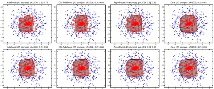
Synthetic data set We first illustrate the effectiveness of our approach on a synthetic data set similar to the one used in [22]. We compare pAUCEns against the baseline Ad-aBoost, Cost-Sensitive AdaBoost (CS-AdaBoost) [14] and Asymmetric AdaBoost (AsymBoost) [22]. We use verti-cal and horizontal decision stumps as the weak classifier. We evaluate the partial AUC score of different algorithms at [0,0.2] FPRs. For each algorithm, we train a strong classifier consisting of 10and25weak classifiers. Addi-tional details of the experimental set-up are provided in the supplementary. Fig. 1 illustrates the boundary decision2 and the pAUC score. Our approach outperforms all other asymmetric classifiers. We observe that pAUCEns places more emphasis on positive samples than negative samples to ensure the highest detection rate at the left-most part of the ROC curve (FPR< 0.2). Even though we choose the asymmetric parameter,k, from a large range of values, both CS-AdaBoost and AsymBoost perform slightly worse than our approach. AdaBoost performs worst on this toy data set since it optimizes the overall classification accu-racy. However as the number of weak classifiers increases (>50stumps), we observe all algorithms perform similarly on this simple toy data set. This observation could explain the success of AdaBoost in many object detection applica-tions even though AdaBoost only minimizes the symmetric error rate.

In the next experiment, we train a strong classifier of10

weak classifiers and compare the performance of different classifiers at FPR of0.5. We choose this value since it is the node learning goal often used in training a cascade clas-sifier. Also we only learn10weak classifiers since the first node of the cascade often contains a small number of weak classifiers for real-time performance. For pAUCEns, we set the value of[α, β]to be[0.49,0.51]. In Fig.2, we display the decision boundary of each algorithm, and display both their pAUC score (in the FPR range [0.49,0.51]) and de-tection rate at50%false positive rate. We observe that our approach and AsymBoost have the highest detection rate at50%false positive rate. However, our approach outper-forms AsymBoost on a pAUC score. We observe that our approach places more emphasis on positive samples near the corners (atπ/4,3π/4,−π/4 and−3π/4angles) than other algorithms.

Protein-protein interaction prediction In this experi-ment, we compare our approach with existing algorithms which optimize pAUC in bioinformatics. The problem

(7)

AdaBoost (10 stumps) pAUC[0, 0.2]: 0.75 −3 −2 −1 0 1 2 3 −2.5 −2 −1.5 −1 −0.5 0 0.5 1 1.5 2 2.5

CS−AdaBoost (10 stumps) pAUC[0, 0.2]: 0.80

−3 −2 −1 0 1 2 3 −2.5 −2 −1.5 −1 −0.5 0 0.5 1 1.5 2 2.5

AsymBoost (10 stumps) pAUC[0, 0.2]: 0.82

−3 −2 −1 0 1 2 3 −2.5 −2 −1.5 −1 −0.5 0 0.5 1 1.5 2 2.5

Ours (10 stumps) pAUC[0, 0.2]: 0.84

−3 −2 −1 0 1 2 3 −2.5 −2 −1.5 −1 −0.5 0 0.5 1 1.5 2 2.5

AdaBoost (25 stumps) pAUC[0, 0.2]: 0.85

−3 −2 −1 0 1 2 3 −2.5 −2 −1.5 −1 −0.5 0 0.5 1 1.5 2 2.5

CS−AdaBoost (25 stumps) pAUC[0, 0.2]: 0.86

−3 −2 −1 0 1 2 3 −2.5 −2 −1.5 −1 −0.5 0 0.5 1 1.5 2 2.5

AsymBoost (25 stumps) pAUC[0, 0.2]: 0.86

−3 −2 −1 0 1 2 3 −2.5 −2 −1.5 −1 −0.5 0 0.5 1 1.5 2 2.5

Ours (25 stumps) pAUC[0, 0.2]: 0.90

−3 −2 −1 0 1 2 3 −2.5 −2 −1.5 −1 −0.5 0 0.5 1 1.5 2 2.5

Figure 1: Decision boundaries on the toy data set where each strong classifier consists ofTop row: 10weak classifiers andBottom row: 25weak

classifiers. Positive and negative data are represented by◦and×, respectively. The partial AUC score in the FPR range[0,0.2]is also displayed. Our approach achieves the best pAUC score of0.84and0.9at10and25weak classifiers, respectively. At25weak classifiers, we observe that both traditional and asymmetric classifiers start to perform similarly.

AdaBoost [email protected]: 0.84, [email protected]: 0.94 −3 −2 −1 0 1 2 3 −2.5 −2 −1.5 −1 −0.5 0 0.5 1 1.5 2 2.5 CS−AdaBoost [email protected]: 0.87, [email protected]: 0.96 −3 −2 −1 0 1 2 3 −2.5 −2 −1.5 −1 −0.5 0 0.5 1 1.5 2 2.5 AsymBoost [email protected]: 0.90, [email protected]: 1.00 −3 −2 −1 0 1 2 3 −2.5 −2 −1.5 −1 −0.5 0 0.5 1 1.5 2 2.5 Ours [email protected]: 0.93, [email protected]: 1.00 −3 −2 −1 0 1 2 3 −2.5 −2 −1.5 −1 −0.5 0 0.5 1 1.5 2 2.5

Figure 2:Decision boundaries on a toy data set with10weak classifiers at FPR of0.5The partial AUC score and detection rate at50%false positive rate

are also shown. Our approach performs best on both evaluation criteria. Our approach preserves a larger decision boundary near positive samples atπ/4,

3π/4,−π/4and−3π/4angles.

we consider here is a protein-protein interaction predic-tion [18], in which the task is to predict whether a pair of proteins interact or not. We used the data set labelled ‘Phys-ical Interaction Task in Detailed feature type’, which is

pub-licly available on the internet3. The data set contains2865

protein pairs known to be interacting (positive) and a ran-dom set of237,384protein pairs labelled as non-interacting (negative). We use a subset of85features as in [16]. We

3_{http://www.cs.cmu.edu/˜qyj/papers_sulp/} proteins05_pages/feature-download.html pAUC(0,0.1) Ours (pAUCEns) 56.05% SVMpAUC[0,0.1]†[16] 54.98% pAUCBoost[0,0.1]††[11] 48.65% Asym SVM[0,0.1]††[28] 44.51% SVM††_AUC[10] 39.72%

Table 1: The pAUC score on Protein-protein interaction data set. The

higher the pAUC score, thebetter the classifier. †The result reported

here is better than the one reported in [16]. We suspect that we tuned the regularization parameter in the finer range. Results marked by††were reported in [16]. The best classifier is shown in boldface.

(8)

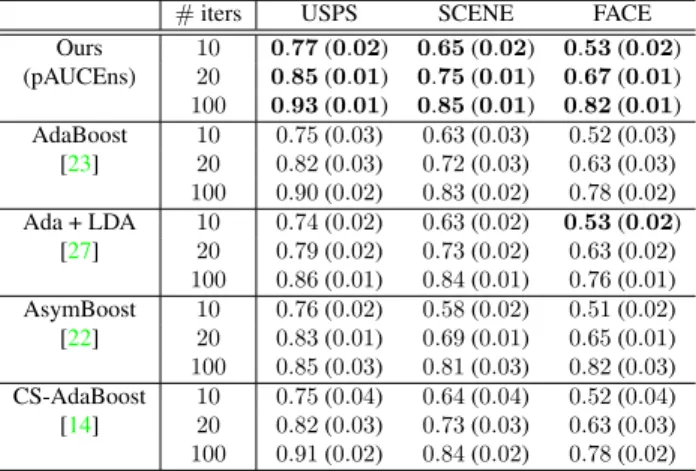
#iters USPS SCENE FACE Ours 10 0.77(0.02) 0.65(0.02) 0.53(0.02) (pAUCEns) 20 0.85(0.01) 0.75(0.01) 0.67(0.01) 100 0.93(0.01) 0.85(0.01) 0.82(0.01) AdaBoost 10 0.75(0.03) 0.63(0.03) 0.52(0.03) [23] 20 0.82(0.03) 0.72(0.03) 0.63(0.03) 100 0.90(0.02) 0.83(0.02) 0.78(0.02) Ada + LDA 10 0.74(0.02) 0.63(0.02) 0.53(0.02) [27] 20 0.79(0.02) 0.73(0.02) 0.63(0.02) 100 0.86(0.01) 0.84(0.01) 0.76(0.01) AsymBoost 10 0.76(0.02) 0.58(0.02) 0.51(0.02) [22] 20 0.83(0.01) 0.69(0.01) 0.65(0.01) 100 0.85(0.03) 0.81(0.03) 0.82(0.03) CS-AdaBoost 10 0.75(0.04) 0.64(0.04) 0.52(0.04) [14] 20 0.82(0.03) 0.73(0.03) 0.63(0.03) 100 0.91(0.02) 0.84(0.02) 0.78(0.02)

Table 2: Average pAUC scores and their standard deviations on vision

data sets at various boosting iterations. All experiments are repeated20

times. The best average performance is shown in boldface.

randomly split the data into two groups: 10% for train-ing/validation and90%for evaluation. We choose the best regularization parameter form{5,2,1,1/2,1/5}by5-fold cross validation. We repeat our experiments10times using the same regularization parameter. We train a linear clas-sifier as our weak learner using LIBLINEAR [8]. We set the maximum number of boosting iterations to100and re-port the pAUC score of our approach in Table1. Baselines include SVMpAUC, SVMAUC, pAUCBoost and

Asymmet-ric SVM. Our approach outperforms all existing algorithms which optimize either AUC or pAUC . We attribute our im-provement over SVMpAUC [0,0.1][16], as a result of

in-troducing a non-linearity into the original problem. This phenomenon has also been observed in face detection as re-ported in [27].

Comparison to other asymmetric boosting Here we compare pAUCEns against several boosting algorithms previously proposed for the problem of object detection, namely, AdaBoost with Fisher LDA post-processing [27], AsymBoost [22] and CS-AdaBoost [14]. The results of Ad-aBoost are also presented as the baseline. For each algo-rithm, we train a strong classifier consisting of100 weak classifiers. We then calculate the pAUC score by varying the threshold value in the FPR range[0,0.1]. For each al-gorithm, the experiment is repeated20times and the aver-age pAUC score is reported. For AsymBoost, we choosek

from{2−0.5,2−0.4,· · ·,20.5}by cross-validation. For CS-AdaBoost, we choosekfrom{0.5,0.75,· · ·,3}by cross-validation. We evaluate the performance of all algorithms on 3 vision data sets: USPS digits, scenes and face data sets. See supplementary for more details on feature extrac-tion. We report the experimental results in Table2. From the table, pAUCEns demonstrates the best performance on all three vision data sets.

Pedestrian detection - Strong classifier We evaluate our approach on the pedestrian detection task. We train our ap-proach on the INRIA pedestrian data set. For the positive training data, we use all 2416INRIA cropped pedestrian images. To generate the negative training data, we first train the cascade classifier with20nodes using Viola and Jones’ approach. We then combine 2416 random negative win-dows generated in the first node with another4832negative windows generated in the subsequent nodes. The resulting

7248negative windows are used for training the strong clas-sifier. We generate a large pool of features by combining the histogram of oriented gradient (HOG) features [3] and co-variance (COV) features4_{[21]. Additional details of HOG} and COV parameters are provided in the supplementary. We use weighted linear discriminant analysis (WLDA) as weak classifiers. We train 500weak classifiers and set 5 multi-exits [17]. To be more specific, we set the threshold at10,

20,50,100and200weak classifiers. These exits reduce the evaluation time during testing significantly. The regulariza-tion parameterνis cross-validated from{0.1,0.5,1,2,10}. Since we have not carefully cross-validated a finer range of

ν, tuning this parameter could yield a further improvement. The training time of our approach is under two hours on a parallelized quad core Xeon machine.

During evaluation, each test image is scanned with4×4

pixels step stride and the scale ratio of input image pyramid is1.05. The overlapped detection windows are merged us-ing the greedy non-maximum suppression strategy as intro-duced in [6]. We use the continuous AUC evaluation soft-ware of Sermanetet al. [19] and report the pAUC score be-tween[0,0.005]FPPI (1false positive), [0,0.05]FPPI (15

false positives),[0,0.5]FPPI (144false positives) and[0,1]

FPPI (288false positives) in Table3. From the table, we ob-serve that setting the value ofβ to be minimal (β = 0.05) yeilds the best pAUC score at[0,0.005]FPPI . As we in-crease the FPPI range, the higher value of β tends to per-form better. This table clearly illustrates the advantage of our approach.

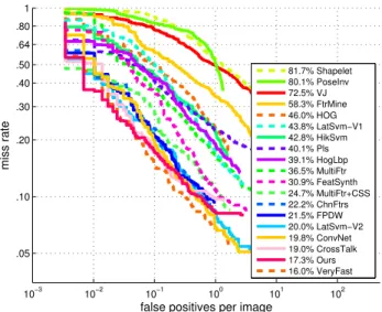
Fig.3 compares the performance of our approach with other state-of-the-art algorithms on the INRIA pedestrian data set. We use the evaluation software of Doll´aret al. [7], which computes the AUC from 9discrete points sampled between[0.01,1.0]FPPI . Our approach performs second best on this data set. It performs comparable to VeryFast [1] which trains multiple detectors at multiple scale. Upon a closer observation, our pAUCEns performs slightly better than VeryFast when the number of FPPI is less then0.1and VeryFast performs slightly better when the number of FPPI is greater0.1. We evaluate our strong classifier on TUD-4_{Covariance features capture the relationship between different image}

statistics and have been shown to perform well in our previous experi-ments. However, other discriminative features can also be used here in-stead,e.g., Haar-like features, Local Binary Pattern (LBP) [15], Sketch Tokens [13] and self-similarity of low-level features (CSS) [24].

(9)

10−3 10−2 10−1 100 101 102 .05 .10 .20 .30 .40 .50 .64 .80 1

false positives per image

miss rate 81.7% Shapelet 80.1% PoseInv 72.5% VJ 58.3% FtrMine 46.0% HOG 43.8% LatSvm−V1 42.8% HikSvm 40.1% Pls 39.1% HogLbp 36.5% MultiFtr 30.9% FeatSynth 24.7% MultiFtr+CSS 22.2% ChnFtrs 21.5% FPDW 20.0% LatSvm−V2 19.8% ConvNet 19.0% CrossTalk 17.3% Ours 16.0% VeryFast

Figure 3:ROC curves of our approach and several state-of-the-art

detec-tors on the INRIA test image. We train a strong classifier using HOG and COV features.

Brussels and ETH pedestrian data sets but we observe that the detection results contain a large number of false posi-tives. Instead of bootstrapping with more negative samples as in [6,24], we train a cascade classifier in the next section.

Pedestrian detection - Cascade classifier In this section, we train a cascade classifier using our pAUCEns. We train our detector on INRIA training set and evaluate the detec-tor on INRIA, TUD-Brussels and ETH test sets. On both TUD-Brussels and ETH data sets, we upsample the original image to 1600×1200 pixels before applying our pedes-trian detector. We train the human detector with a combi-nation of HOG and COV features as previously described. To achieve the node learning goal of the cascade (each node achieves an extremely high detection rate (> 99%) and a moderate false positive rage (≈ 50%)), we optimize the pAUC in the FPR range[0.49,0.51]. We train a multi-exit cascade [17] with19 exit. In this experiment, we use the software of [19] to compute the continuous AUC score in the FPPI range[0,0.1]. We sort different algorithms based

on the pAUC score in the FPPI range[0,0.1]and report the results in Fig.4. We compare our proposed approach with the baseline HOGCOV classifier (using AdaBoost). We ob-serve that our approach reduces the average miss-rate over HOGCOV by7%on INRIA test set. From Fig.4, our ap-proach achieves similar performance to the state-of-the-art detector. We then break-down experimental results of dif-ferent measures using the partial AUC score (FPPI range

[0,0.1]) in Table4. On average, our approach performs best on thelargeevaluation setting where pedestrians are at least

100pixels tall. On other settings, our approach yields com-petitive results to the state-of-the-art detector in that cate-gory. In summary, our approach performs better than or on par with the state-of-the-art despite its simplicity (in com-parison to LatSvm — a part-based approach which models unknown parts as latent variables). In addition, the current detector is only trained with two discriminative visual fea-tures (HOG and COV). Applying additional discriminative features,e.g., LBP [26] or motion features [24], could fur-ther improve the overall detection performance.

4. Conclusion

We have proposed a new ensemble learning method for object detection. The proposed approach is based on op-timizing the partial AUC score in the FPR range [α, β]. Extensive experiments demonstrate the effectiveness of the proposed approach in visual detection tasks. We plan to ex-plore the possibility of applying the proposed approach to the multiple scales detector of [1] in order to improve the detection results of very low resolution pedestrian images.

References

[1] R. Benenson, M. Mathias, R. Timofte, and L. V. Gool. Pedes-trian detection at 100 frames per second. InProc. IEEE Conf. Comp. Vis. Patt. Recogn., 2012.7,8

[2] R. Benenson, M. Mathias, T. Tuytelaars, and L. V. Gool. Seeking the strongest rigid detector. InProc. IEEE Conf. Comp. Vis. Patt. Recogn., 2013.2

[3] N. Dalal and B. Triggs. Histograms of oriented gradients for human detection. InProc. IEEE Conf. Comp. Vis. Patt. Recogn., volume 1, 2005.7 Train Test (FPPI) [0,0.005] [0,0.05] [0,0.5] [0,1] β= 0.05 65.0% 39.3% 20.6% 18.1% β= 0.1 75.7% 32.5% 18.0% 15.8% β= 0.5 73.4% 33.8% 17.9% 15.3%

Table 3:The pAUC score in the FPR range[0, β]on the training set. Our

objective here is to optimize the area under the curve between[0,0.005],

[0,0.05],[0,0.5]and[0,1]FPPI on the INRIA test set. Since we plot FPPI versus miss rate, asmaller pAUC scoremeans abetter detector. The best detector at each FPPI range is shown in boldface. Clearly, a large value ofβis best for a large FPPI range.

(10)

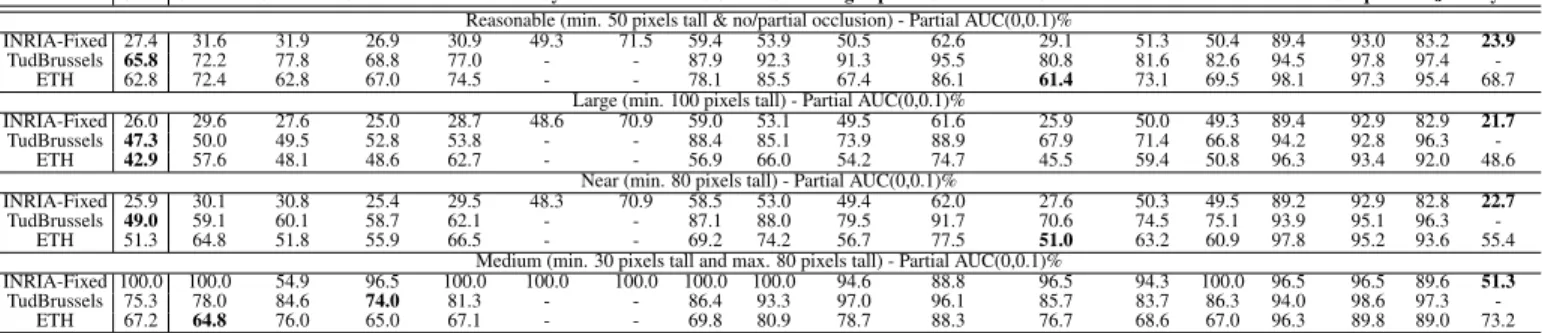
Ours ChnFtrs ConvNet CrossTalk FPDW FeatSynth FtrMine HOG HikSvm HogLbp LatSvm-V1 LatSvm-V2 MultiFtr Pls PoseInv Shapelet VJ VeryFast Reasonable (min. 50 pixels tall & no/partial occlusion) - Partial AUC(0,0.1)%

INRIA-Fixed 27.4 31.6 31.9 26.9 30.9 49.3 71.5 59.4 53.9 50.5 62.6 29.1 51.3 50.4 89.4 93.0 83.2 23.9 TudBrussels 65.8 72.2 77.8 68.8 77.0 - - 87.9 92.3 91.3 95.5 80.8 81.6 82.6 94.5 97.8 97.4

-ETH 62.8 72.4 62.8 67.0 74.5 - - 78.1 85.5 67.4 86.1 61.4 73.1 69.5 98.1 97.3 95.4 68.7 Large (min. 100 pixels tall) - Partial AUC(0,0.1)%

-ETH 42.9 57.6 48.1 48.6 62.7 - - 56.9 66.0 54.2 74.7 45.5 59.4 50.8 96.3 93.4 92.0 48.6 Near (min. 80 pixels tall) - Partial AUC(0,0.1)%

-ETH 51.3 64.8 51.8 55.9 66.5 - - 69.2 74.2 56.7 77.5 51.0 63.2 60.9 97.8 95.2 93.6 55.4 Medium (min. 30 pixels tall and max. 80 pixels tall) - Partial AUC(0,0.1)%

-ETH 67.2 64.8 76.0 65.0 67.1 - - 69.8 80.9 78.7 88.3 76.7 68.6 67.0 96.3 89.8 89.0 73.2

Table 4:Performance comparison of various detectors on several pedestrian test sets. The best detector in each category from each data set is highlighted

in bold. The AUC score is taken over the FPPI range[0,0.1]. Asmaller pAUC scoremeans abetter detector. The AUC score over the FPPI range[0,1]

can be found in the supplementary.

[4] A. Demiriz, K. Bennett, and J. Shawe-Taylor. Linear pro-gramming boosting via column generation. Mach. Learn., 46(1–3):225–254, 2002.4

[5] L. E. Dodd and M. S. Pepe. Partial auc estimation and re-gression.Biometrics, 59(3):614–623, 2003.3

[6] P. Doll´ar, Z. Tu, P. Perona, and S. Belongie. Integral channel features. InProc. of British Mach. Vis. Conf., 2009.5,7,8 [7] P. Doll´ar, C. Wojek, B. Schiele, and P. Perona. Pedestrian

detection: An evaluation of the state of the art. IEEE Trans. Pattern Anal. Mach. Intell., 34(4):743–761, 2012.1,7 [8] R.-E. Fan, K.-W. Chang, C.-J. Hsieh, X.-R. Wang, and C.-J.

Lin. LIBLINEAR: A library for large linear classification.J. Mach. Learn. Res., 9:1871–1874, 2008.7

[9] M.-J. Hsu and H.-M. Hsueh. The linear combinations of biomarkers which maximize the partial area under the roc curves.Comp. Stats., 28(2):1–20, 2012.2

[10] T. Joachims, T. Finley, and C.-N. J. Yu. Cutting-plane train-ing of structural svms.Mach. Learn., 77(1):27–59, 2009.4, 6

[11] O. Komori and S. Eguchi. A boosting method for maximiz-ing the partial area under the roc curve.BMC Bioinformatics, 11(1):314, 2010.2,6

[12] O. Komori and S. Eguchi. Boosting learning algorithm for pattern recognition and beyond. IEICE Trans. Infor. and Syst., 94(10):1863–1869, 2011.4

[13] J. J. Lim, C. L. Zitnick, and P. Dollar. Sketch Tokens: A learned mid-level representation for contour and object de-tection. InProc. IEEE Conf. Comp. Vis. Patt. Recogn., 2013. 7

[14] H. Masnadi-Shirazi and N. Vasconcelos. Cost-sensitive boosting. IEEE Trans. Pattern Anal. Mach. Intell., 33(2):294–309, 2011.2,5,7

[15] Y. Mu, S. Yan, Y. Liu, T. Huang, and B. Zhou. Discriminative local binary patterns for human detection in personal album. InProc. IEEE Conf. Comp. Vis. Patt. Recogn., Anchorage, AK, US, 2008.7

[16] H. Narasimhan and S. Agarwal. A structural svm based ap-proach for optimizing partial auc. InProc. Int. Conf. Mach. Learn., 2013.2,3,4,5,6,7

[17] M.-T. Pham, V.-D. D. Hoang, and T.-J. Cham. Detection with multi-exit asymmetric boosting. InProc. IEEE Conf. Comp. Vis. Patt. Recogn., 2008.7,8

[18] Y. Qi, Z. Bar-Joseph, and J. Klein-Seetharaman. Evaluation of different biological data and computational classification methods for use in protein interaction prediction. Proteins: Struct., Func., and Bioinfor., 63(3):490–500, 2006.6 [19] P. Sermanet, K. Kavukcuoglu, S. Chintala, and Y. LeCun.

Pedestrian detection with unsupervised multi-stage feature learning. In Proc. IEEE Conf. Comp. Vis. Patt. Recogn., 2013.7,8

[20] C. Shen, P. Wang, S. Paisitkriangkrai, and A. van den Hen-gel. Training effective node classifiers for cascade classifica-tion.Int. J. Computer Vision, 103(3):326–347, 2013.2 [21] O. Tuzel, F. Porikli, and P. Meer. Pedestrian detection via

classification on Riemannian manifolds.IEEE Trans. Pattern Anal. Mach. Intell., 30(10):1713–1727, 2008.7

[22] P. Viola and M. Jones. Fast and robust classification us-ing asymmetric AdaBoost and a detector cascade. InProc. Adv. Neural Inf. Process. Syst., pages 1311–1318. MIT Press, 2002.2,5,7

[23] P. Viola and M. J. Jones. Robust real-time face detection.Int. J. Comp. Vis., 57(2):137–154, 2004.1,5,7

[24] S. Walk, N. Majer, K. Schindler, and B. Schiele. New fea-tures and insights for pedestrian detection. InProc. IEEE Conf. Comp. Vis. Patt. Recogn., San Francisco, US, 2010. 7, 8

[25] P. Wang, C. Shen, N. Barnes, and H. Zheng. Fast and robust object detection using asymmetric totally-corrective boost-ing. IEEE Trans. Neural Networks and Learning Systems, 23(1):33–46, 2012.2

[26] X. Wang, T. X. Han, and S. Yan. An HOG-LBP human de-tector with partial occlusion handling. InProc. IEEE Int. Conf. Comp. Vis., 2009.8

[27] J. Wu, S. C. Brubaker, M. D. Mullin, and J. M. Rehg. Fast asymmetric learning for cascade face detection.IEEE Trans. Pattern Anal. Mach. Intell., 30(3):369–382, 2008.5,7 [28] S.-H. Wu, K.-P. Lin, C.-M. Chen, and M.-S. Chen.

(11)

10−2 10−1 100 101 102 .05 .10 .20 .30 .40 .50 .64 .80 1

miss rate 94.6% Shapelet 90.0% PoseInv 84.4% VJ 73.0% FtrMine 64.1% LatSvm−V1 60.5% HOG 56.4% HikSvm 53.1% HogLbp 52.3% Pls 52.2% MultiFtr 49.4% FeatSynth 36.8% MultiFtr+CSS 34.9% HOGCOV 33.6% ChnFtrs 33.2% ConvNet 32.4% FPDW 29.8% LatSvm−V2 28.0% CrossTalk 27.4% Ours 25.3% VeryFast 10−3 ₁₀−2 ₁₀−1 ₁₀0 ₁₀1 ₁₀2 .30 .40 .50 .64 .80 1

miss rate 98.2% Shapelet 97.8% VJ 96.1% LatSvm−V1 95.5% PoseInv 93.5% HikSvm 93.0% HogLbp 89.9% HOG 85.8% Pls 85.0% MultiFtr 84.5% LatSvm−V2 82.1% ConvNet 81.3% FPDW 77.3% ChnFtrs 75.3% MultiFtr+CSS 74.4% CrossTalk 71.4% MultiFtr+Motion 71.4% Ours 10−3 10−2 10−1 100 101 102 .20 .30 .40 .50 .64 .80 1

miss rate 98.3% PoseInv 97.6% Shapelet 95.6% VJ 87.5% LatSvm−V1 86.3% HikSvm 82.2% MultiFtr+Motion 82.1% MultiFtr+CSS 80.0% HOG 77.8% FPDW 75.9% MultiFtr 75.8% ChnFtrs 73.4% Pls 72.6% VeryFast 72.2% HogLbp 70.6% CrossTalk 68.5% ConvNet 67.8% Ours 67.3% LatSvm−V2

Figure 4:From top to bottom: performance on INRIA, TUD-Brussels and

ETH test set. Algorithms are sorted using thepartial AUC scorein the FPPI range[0,0.1]. Our pAUCEns consistently performs comparable to the state-of-the-art.

under the user tolerance. InProc. of Intl. Conf. on Knowl-edge Discovery and Data Mining, 2008.2,6