PICav: Precise, Iterative and Complement-based
Cloud Storage Availability Calculation Scheme
Josef Spillner, Johannes Müller
Technische Universität DresdenFaculty of Computer Science Cloud Storage Lab (lab.nubisave.org)
01062 Dresden, Germany
Email: [email protected], [email protected]
Abstract—Cloud storage controllers combine multiple hetero-geneous storage services into a unified virtual storage area for users. The overall storage quality depends on all the individual service qualities as well as on the controller’s ability to mitigate quality issues, for instance with caches and proper scheduling to improve the availability of data. Given a set of storage services with an estimated capacity and average availability for each, the problem arises how to distribute the data and which amount of redundancy needs to be generated in order to maintain a certain overall availability. There are few previous algorithm proposals for this computationally hard problem which produce high transmission overhead and imprecise results. We present a novel algorithm which minimises the overhead and achieves exact values in short time. Furthermore, our algorithm takes storage service interdependencies into account. We validate our claims with synthetic failure distributions and real traces from three cloud services.
I. PROBLEMSTATEMENT
Pervasive data access across devices and services with-out worries abwith-out insecurity or unavailability is one of the promises of cloud storage proponents. The solutions which come closest to this vision are typically combining multiple storage services, partitioning and splitting data to be stored among them with a certain added redundancy [1], [2]. The amount of redundancy influences the overall availability of data in case of service failures. If data is split into two halves with 50% added redundancy, and stored across three services (on independent storage nodes) with 98% estimated availabil-ity for each, this scheme results in an overall availabilavailabil-ity equal to 99.88% compared to only 96% without the redundant node. In practice, both the availabilities (a) and the capacities (c) of online storage services differ significantly and cannot be assumed to be equal. Table I lists a few popular free and paid services with their characteristics collected from different sources. An unavailability of 0.1% translates into 43:48 minutes per month on average. Furthermore, retrieval and restore times differ as well and additionally depend on the user’s network connection. Registries, brokers and marketplaces are used by storage controllers to dynamically select suitable services based on their properties although they suffer from incomplete and out of date information [3]. The optimal selection for a user, based on their capacity requirements and a presumed always-available overall service quality, can nevertheless be matched closely with a selection
from the marketplaces. This results in heterogeneous sets ofn
out ofhavailable storage services to whichk significant and
mredundant data fragments are assigned.
TABLE I
STORAGE SERVICES CHARACTERISTICS Service Capacityc Availabilitya
Google Drive 15 GB 99.9% (SLA)
Amazon S3 on-demand 99.9% (SLA), 98.86% in July 2008 AT&T on-demand 99.5% (Nasuni study 2011)
Linode 1-96 GB 99.951% (CloudHarmondy study 2011) iCloud 5 GB 99.65% (Cérin et al. 2012 [4])
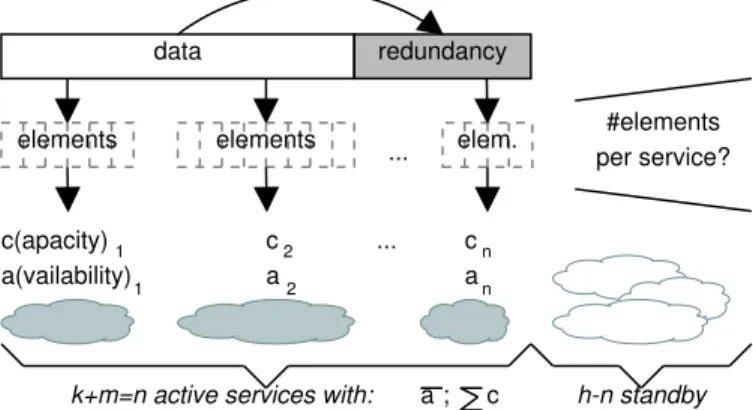
With such diverse settings, determining the right amount of redundancy becomes challenging. Given the previous example, it would be possible to increase the amount of redundancy to 60% with erasure coding. Unless the number of independent storage services also increases, there would however be no gain in availability. The problem is explained in its general form in Fig. 1. c(apacity) a(vailability) c a c a ... 1 2 n 2 n data redundancy ... #elements per service? 1
k+m=n active services with: h-n standby
elements elements elem.
a; c
Fig. 1. Problem definition for a set of heterogeneous storage services with varying availabilities and capacities; not considering cost or other properties
Research into optimal distribution of erasure-coded data to storage services with heterogeneous availabilities suggests to generate a fixed number of e.g. n = 100 equally-sized ele-ments (fragele-ments), which is significantly larger than the num-ber of storage services, and distribute the individual elements proportionally to the availabilities [5]. This rather simple strategy can lead to up to 70% redundancy savings, without the
overhead of having to search a large multidimensional space. Three problems arise when applying this strategy in a cloud storage environment. First, encoded data is split into numerous files, which results in a multiplication of network overhead per storage service. Second, when working with small files, there may be a storage overhead. For instance if we use a word size of w = 8 and a packet size packetsize = 512bytes, each element is at leastelementsizemin=w∗packetsize=
4096byteslarge. Assuming we work on a file of f ilesize= 100bytes, the overhead isoverhead=n∗elementsizemin−
100bytes = 409.5KB. To avoid the first problem, instead of producing many small files, the resulting elements per service are assembled into a single file for the transmission process which can be split back into separate elements before decoding. Further, to reduce overhead, the packetsize and
wordsizeparameters are minimised. This leads to a decrease in throughput as shown in [6]. The third remaining problem is a lack of precision for the global availability results. To counter the performance loss, further decrease overhead by reducing the number of erasure code elements, and gain precision as well, we propose a novel element distribution algorithm called PICav. We show that PICav can be used to quickly generate fragment distributions with similar availability compared to the proportional distribution of a high number of elements, while at the same time showing improved throughput and higher precision.
II. ALGORITHMDESCRIPTION
We pursue the construction of the PICav algorithm as follows: First, we outline our assumptions and the model which is constrained by them. Then, we present the calculation scheme. For completeness, we look at service dependency and recovery aspects before finally evaluating the scheme.
A. General Considerations
The cloud storage model consists of n mostly indepen-dent storage services, each with an estimated value for data availability a. It assumes that availability of data can only be impaired by a failure that causes a service to be offline or its data to be lost or corrupted. Thus, availability is the ratio of time when the service’s data is accessible to the time it is inaccessible. Accessibility here means that the original data can be retrieved. In general, the term availability may be defined more broadly and include further end-to-end resource uncertainty factors such as corrupt network routes or slow responses. The interpretation of these factors is implementation-dependent (e.g. timeouts in the transport connectors, multipath connections, caching) and hence omitted from our model although we will discuss their influence in the discussion section. The availability is often an approximate value that may be determined empirically by reading and verifying the data in a periodic monitoring process, or by comparing the service to similar ones with a known availabil-ity. The resulting value is used as input to predict the actual availability in the future. The binary states {available, unavailable} follow a stochastic distribution. According
to previous analyses, incidents are mostly temporal and the availability is generally high [7]. A Weibull distribution, a more specific exponential distribution, as well as normal and beta distributions can be found in the literature to describe the nature of service availabilities over time. We will first follow the previous work in assuming a beta distribution [5] but then argue for a normal distribution as well, which yields better results. An additional assumption is that the user is interested in the minimum availability instead of the mean one, and that the erasure-coded data is distributed with a parallel scheduling as opposed to, for instance, round-robin distribution. This restriction, too, will be elaborated on in the discussion section. We informally derive the availability calculation in Eq. 1. A more formal definition is given in other works, e.g. [5].
First,Cis the combination of thenservicesswhich is used to store data. Second, the powersetP(C)of this combination is calculated. Third, the powerset is filtered so that it merely contains all combinations of services with enough chunks to restore the original data. This filtered set is referred to as
Pf(C)and represents every possible combination of services that suffices to restore the original data. Therefore, the minimal availability of data is the probability of at least one subset of services Sj∈ Pf(C)to be available. Further, the availability
ais the sum of the set probabilities aj for each combination
Sj to be available exclusively. This means that the services
sj,k ∈ Sj are available, while the other services in C are unavailable. Consequently, aj is the multiplication of the availability of each serviceaj,kmultiplied by the probabilities
uj,l for the other services in Tj ∈C\Sj to be unavailable. The unavailabilityuj,lis the multiplication of the complement of the availability of each service inTj. IfTj is empty,aj is simply the multiplication of the availability of each service
aj,k, since every service in the term Tj is unavailable with absolute certainty. Like in the formula before, it is assumed that each of the sets and subsets of services previously discussed is substituted by a multiset with the availabilities of the services in the respective set or subset. For the case thatC\S in the formula, which corresponds toTj, is empty, the product over the thereby empty set is defined as one.
availability= X S∈Pf(C) Y a∈S a· Y u∈{1−ub|ub∈(C\S)} u (1) B. Calculation Scheme
The proposed availability calculation scheme is charac-terised by yielding precise values on the visible interface level and by being iterative and working on availability complement values in its implementation. Hence, we call it a precise, iterative and complement-based scheme (PICav).
The use of complements leads to a higher performance. It marks an improvement in the algorithm used to calculate avail-ability for a set of heterogeneous storage nodes, decreasing worst case and average complexity by half. This is sufficient to calculate availabilities for configurations with less than 30 nodes, which enables the user interfaces of storage controllers
to respond fluently to changes in the configuration. We assume fixed parameters n andk for the erasure code. Colloquially, as presented before, availability is calculated as the sum of probabilities of all storage node combinations which suffice to reconstruct the original data, whereas a combination’s probability is the probability that each of its stores is on-line while the others are off-on-line. The complexity of O(2n) with n being the number of nodes is due to the growth in possible combinations that need to be considered. The worst case occurs whenmis largest, i.e. many redundant nodes can be excluded. To decrease the number of nodes that need to be considered when determining overall availability, we propose to calculate the complement of the availability when k is smaller than n2, and then simply inferring the availability from this result. To calculate unavailability, we simply substitute the set of combinations in the previous calculation with the set of combinations that store less than k blocks. More precisely, we add up all probabilities of all storage node combinations that are not sufficient for data reconstruction. With this, we decrease the number of combinations that need to be considered, and thus reduce the algorithm worst case runtime by half. For 30 storage nodes or more, we implement the calculation for storage services with homogeneous availability, which is not as accurate, but more scalable [5].
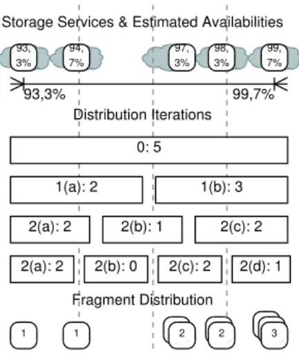
The subsequent iterative distribution algorithm increases the number of elements according to the variance in availability. First, it starts at distributing one element to each service, which is optimal in the homogeneous case. Services are divided into a growing number of separate classes according to their availability. To this end, we define an interval of availabilities for each class. The first single interval is exactly between the lowest and highest availability of all services. If possible, this single interval is divided in two, three, four and more evenly sized intervals, each corresponding to a separate class of nodes with the according availabilities. The algorithm adds one element to the nodes in the first non-empty class, two to the second, three to the third, and so on. The separation into more classes stops if we have reached a fixed number of elements, which we set to 30 in our approach. It starts with choosing the first variation, and only takes the next variation if it increases availability, and if it monotonically converges against the desired redundancy.
Fig. 2 presents a graphical explanation of how the algo-rithm works with an example of five storage services which have a wide range of availabilities for didactic purposes. It ultimately results in splitting the data into 9 fragments which are distributed unevenly over the five services.
C. Service Dependencies
We extend the model to calculate data availability in order to consider single uni-directional dependencies between storage services. For instance, Dropbox and Ubuntu One depend on Amazon’s S3 storage. We assume that if Amazon S3 is unavailable, Dropbox is unavailable as well. The error introduced by ignoring such dependencies can be considerable. For instance, if we replicate data to Amazon S3 and Dropbox
Storage Services & Estimated Availabilities
93,3% 99,7% 93, 3% 99, 7% 94, 7% 98, 3% 97, 3% Distribution Iterations 1(a): 2 1(b): 3 2(a): 2 2(b): 1 2(c): 2 2(a): 2 2(b): 0 2(c): 2 2(d): 1 Fragment Distribution 1 1 2 2 3 0: 5
Fig. 2. Iterative distribution algorithm
with availabilities of 99.9% and 99% respectively, the overall availability is actually 99.9%, instead of 99.99%. Further, we use knowledge of interdependencies to reduce redundancy. For example, if we have 10 services with a homogeneous availability of 90%, we need to store 2.5 times the amount of the original data to achieve an availability greater than 99.999%. If one of the services depends on an other one, the redundancy factor to achieve this availability is about 3.333. Thus, by using only services without interdependencies, we can reduce the storage cost by about 25%.
D. Retrieval and Recovery
After optimising storage cost with respect to a desired avail-ability, other optimisation goals like cost reduction and storage capacity utilisation shall be pursued. The retrieval extension to PICav reduces cost for data transfer by preferring nodes that produce no or little additional cost for data downloads. Many cloud storage providers like Dropbox, Sugarsync, or TelekomCloud do not bill the user for downloading data, whereas Amazon S3 bills about 12 ¢ per downloaded GB1. Thus, only downloading from the former services does not involve additional costs. Further, when a storage has reached its capacity, the scheme automatically tries to find a suitable substitute from a preconfigured set of services, in order to maintain the desired availability. Otherwise, not all storage space could be used, considering services with different capac-ity limits, since one of the services would reach its limit before the others, or due to storing more data per file according to the erasure code distribution policy. Similar mechanisms can be applied to increase performance by substituting or excluding components exhibiting low throughput.
When a data storage service in our model fails for a long time, we can consider it to have failed permanently. For this case we propose a strategy to reconstruct the lost data to uphold the availability goal, and to protect against possible data loss. Nonetheless, we first need to restore the goal availability value for new data. Three practical examples,
based on experience with SugarSync and Dropbox, serve to illustrate how such data loss might be possible with current cloud storage providers. First, SugarSync deletes free accounts that were not used frequently with an email warning seven days prior to the deletion: You haven’t used your SugarSync account for more than three months. SugarSync regularly deletes accounts which have been inactive for more than three months.If a user does not check notification e-mails often enough, or if the email is accidentally deleted by a spam filter, account data will be lost. Second, SugarSync recently abandoned continuous free of charge service, pressing users to move to a paid account to maintain full access to SugarSync. Third, Dropbox states similar terms of service, stating that they might delete accounts after 12 month of account inactivity2. To prevent data loss, we first increase redundancy. However, using this approach, we can only increase availability until we have a replica of the original data on each service, which might not suffice to restore the goal value for data availability. Another drawback of this approach is that data migration is generally more expensive when the redundancy comes closer to its maximum. Further, when accessing large files, we cannot combine the bandwidth of several providers to increase throughput, since in the worst case, one replica needs to pass through the connection of one provider alone. Therefore, we consider adding one or several new services to the storage array, to keep the number of storage nodes constant over time. The second approach alone may not be able to restore the desired data availability for new data if the additional storage service’s availability is lower than that of its predecessor. Thus, we combine it with the first approach by gradually increasing redundancy after adding another service to the storage array. If another storage service becomes available, we may repeat this process until the goal availability value is met. Apart from better performance, and less migration costs, we assume that in practical scenarios it is often possible to meet the goal availability by dispersing data to more nodes. This hypothesis is supported by the results of [5] which compares redundancy savings in multiple scenarios with 10 and 100 nodes, and by our own experience. Just in case though, we evaluate the results of integrating a new storage to exclude solutions that add more redundancy than needed in the scenario before the node failure, if it is feasible. After having restored an environment that meets the goal data availability, we need to restore the lost data. We could use regenerating erasure codes for more efficient reconstruction compared to using the regular Cauchy-Reed-Solomon (CRS) code. However, most regenerating codes do not reduce the number of elements that need to be accessed, but rather reduce I/O operations. As the transport layer transfers elements atomically such a scheme is inapplicable. Bandwidth saving regenerating codes might require the storage provider to process data before sending them, which makes them inapplicable for general cloud
2Dropbox ToS: https://www.dropbox.com/terms
storage. NCCloud’s functional minimum-storage regenerating code implementation (F-MSR) comes closest in terms of desired properties [8]. Next to being maximum-distance separable (MDS), it can reconstruct data by accessing one of two fixed size regions in an element. Thus, we could separate every element in two, to reduce repair bandwidth by about 25% to 50%. Despite these advantages, there are numerous reasons not to use F-MSR. First, it only offers to tolerate two element failures, even though first approaches exist to tolerate more erasures, such as Xorbas [9]. Due to the improvements coming with PICav, F-MSR cannot effectively be used to reduce repair traffic. In particular, since we operate on up to n = 100 elements, the F-MSR implementation could not provide enough redundancy, as it only considers two element failures. Further, dividing the 100 elements in two would lead to an enormous network overhead. Even when we forfeit our approach, we would still have twice as many files to store, which even without F-MSR proved to be a performance bottleneck. Therefore, we propose complementary improvements in the transport layer to assemble collections of several elements (small files) into archives which are represented as one large file per service before transferring them to the services. Consequently, the elements that were split in two for the sake of reducing repair bandwidth would not be transferred individually anyway. To still decrease repair cost, we propose the following scheme. We increase the number of elements, as well as the number of coding elements by one. Then we store one of the data elements on the local hard disk. When a node fails permanently, we can use the local data elements to replace the data on the failed storage. This approach has the drawback that it can only be used once during the overall lifetime of the data. Nonetheless, it improves repair bandwidth dramatically considering that the minimal amount of data needs to be transferred for reconstruction. Furthermore, it only needs to be uploaded to the new service, so that the bandwidth and performance of the unaffected services are not further impaired by reconstruction, which should allow for normal operation during repair. Once the repair is finished, we could start to restore the previous situation, which would involve reading and replacing the whole data set file by file, which might in turn be quite expensive considering high transfer costs. Nevertheless, this reconstruction can take place while the system is under low load, and might be spread over a long period of time in order to maintain system performance. Also, considering permanent loss unlikely, the potential cost for this reconstruction process might still be sensible.
III. EXPERIMENTALEVALUATION
The evaluation consists of two parts. First, we implemented PICav as a standalone script to verify the numerical results, and integrated the implementation into a storage controller. Then, we performed a number of experiments based on this implementation to check the availability gain and the corresponding reduction in elements.
A. Implementation Description
We have implemented PICav into NubiSave, an open source cloud storage controller [2]. Its configuration GUI now allows users to define a goal availability and to derive the splitting and redundancy configuration in real-time. Furthermore, the suggested transport layer improvements were integrated into CloudFusion, a connector to various popular cloud storage services. A screenshot of the configuration dialogue is shown in Fig. 3.
Fig. 3. The NubiSave configuration GUI with minimum redundancy derived from the availability goal
The standalone script availability.py has been im-plemented in Python. It is invoked with two parameters: The number of significant fragments k, and a list of tuples/triples which represent the storage services. Each tuple contains the estimated availability and the number of erasure code elements. Service dependencies result in a lifting to a triple by adding the tuple position of the dependendee service, starting at 1. Thus, a sample invocation for three services would be python availability.py 2 "[(0.5,3), (0.5,1,0), (0.6,1,1)]" resulting in a = 0.5. The script is publicly available from the NubiSave Git repository [2].
B. Experiments Results
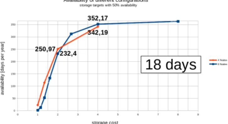
Our experiments work has been initiated with an availability gain analysis. In Fig. 4, which exemplifies storage services with 50% availability, it becomes apparent that already with two redundant elements, the difference in overall availability is 18 days, or 7.99%, when using only four nodes instead of eight.
Fig. 5, Fig. 6, Fig. 7, and Fig. 8 compare our proposed algo-rithms and the proportional distribution directly, by displaying the difference in achieved availability, and the difference in the number of erasure code elements in separate charts with varying values for the variance in availabilities. We generate node availabilities for 10 stores 100 times, using the beta distribution implementation from the Python standard library3.
The experiment uses the same mean availabilities and vari-ances from [5], translating them into the corresponding alpha
3https://docs.python.org/2/library/random.html
Fig. 4. Potential gains when calculating the overall availability
and beta values by using the definition of mean and variance for beta distributions from [10]. Instead of only considering the results for availabilities 0.9, 0.99, and 0.999, we show the complete spectrum of achieved availability between a redundancy of 5, and 10 time replication. The value for a replication factor of ten is omitted, as the optimal distribution for ten storage targets in this case is having one replica per storage, which is achieved by our distribution scheme, since the novel algorithm considers a homogeneous distribution first. The generated tables actually encompass the complete range, beginning with the redundancy of a single replica up to but not including a redundancy factor of ten. But since the achieved availability varies greatly at low redundancy, the comparatively small difference between a redundancy factor of five and ten becomes invisible in the complete figures. For this reason, only the partial diagrams are shown with redundancy of five or more.
To use more comprehensible units than availability percent-age, the charts show the availability gain of using the novel distribution strategy in seconds per year, assuming a year has 31556952 seconds. The y-axis is used to map the different variances into a three dimensional graph, to view the effect of changed variances immediately, except for Fig. 8, which uses the y-axis to display the corresponding pair of mean and variance values. The mapping of several similar configura-tions leads to a more compact representation. To visualise differences despite the distortion caused by the 3D view, a colour coded plane is drawn, which passes through ever point of the individual curves for each mean value, and variance pair. The actual functions are discontinuous, as they do not have a corresponding availability for every redundancy factor. Nonetheless, the charts show them as continuous functions by using the achieved availability for a redundancy closest, but less than or equal to the current redundancy factor.
Fig. 5, Fig. 6, and the simulation of Skype traces in Fig. 8 show that our algorithm performs much worse for availabilities lower than 0.5 between a redundancy factor of 7 and 10. The results for stores with higher availabilities, which is the case for the mean availability of 0.75 displayed in Fig. 7, the results generated for the mean availability and variance
5 6 7 8 9 10 0.01 0.02 0.03 0.04 -1e+06 -500000 0 500000 1e+06 1.5e+06 2e+06
Availability Gain [s/year]
Redundancy Factor Variance -1e+06 -500000 0 500000 1e+06 1.5e+06 2e+06 5 6 7 8 9 10 0.01 0.02 0.03 0.04 -20 -19 -18 -17 -16 -15 -14 Reduction in Elements Redundancy Factor Variance -20 -19 -18 -17 -16 -15 -14
Fig. 5. Availability gain compared to proportional distribution of 30 erasure code elements with corresponding reduction in used erasure code elements for 10 nodes with mean availability of 0.25, and different variances
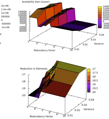
from traces of PlanetLab, and Microsoft, are nearly equal to the proportional distribution strategy, differing only by a few minutes of availability per year, which is less than 0.01% of availability. In case of the simulation for PlanetLab, there is an increase of availability by about one minute. In every case, our novel algorithm succeeds in decreasing the average number of erasure code elements by at least 14, which is nearly half the number of elements. Interestingly, especially when using low redundancy, the achieved availability of both strategies can be several days worse or better, whereas between a redundancy factor of seven and ten, the average results do not fluctuate much, as the maximum possible availability for each strategy has already been achieved.
The proportional distribution policy was applied with only 30 erasure code elements, in order to better compare the results, and because previous work by the same authors suggests that 30 elements is a good choice in their testing environment [11]. Nonetheless, we also re-ran all experiments with 100 erasure code elements. As the results do not differ significantly from the current results except for the obvious increase of required elements for the proportional strategy, we omit a detailed presentation.
5 6 7 8 9 10 0.01 0.02 0.03 0.04 -60000 -40000 -200000 20000 40000 60000 80000 100000 120000 140000
Availability Gain [s/year]
Redundancy Factor Variance -60000 -40000 -20000 0 20000 40000 60000 80000 100000 120000 140000 5 6 7 8 9 10 0.01 0.02 0.03 0.04 -20 -19 -18 -17 Redundancy Factor Variance Reduction in Elements -20 -19.5 -19 -18.5 -18 -17.5 -17
Fig. 6. Availability gain compared to proportional distribution of 30 erasure code elements with corresponding reduction in used erasure code elements for 10 nodes with mean availability of 0.5, and different variances
IV. DISCUSSION
Finding a good configuration for erasure code parameters, and erasure code element distribution for satisfying a cer-tain availability is hard for a user, especially if she is not acquainted to erasure codes and the term availability. For higher transparency, NubiSave represents these statistics in more established units like unavailability in time per year or a redundancy factor, which describes how much redundancy is used compared to using a single replica. A user can easily play around with a redundancy slider, which covers a meaningful range of different redundancy values for each strategy. More-over, to give the user a good starting point, NubiSave needs to provide an automatic search, that chooses the best storage strategy with the lowest redundancy to achieve a desired availability, so that a user can simply state the upper bound for unavailability in percent or in time per year i.e. 0.01% or 5 minutes. This can easily be done, by letting the GUI iterate over the possible configurations for each storage strategy, and finding the best fit. To gain more comparable results, we eval-uated our redundancy scheme by using the beta distribution to generate random node availabilities, as the same distribution is used by the authors proposing the proportional redundancy scheme. It seems that the beta distribution generates rather heterogeneous availabilities despite of a low variance. It would
5 6 7 8 9 10 0.01 0.02 0.03 0.04 -300 -200 -1000 100 200 300 400 500 Redundancy Factor Variance Availability Gain [s/year]
-300 -200 -100 0 100 200 300 400 500 5 6 7 8 9 10 0.01 0.02 0.03 0.04 -20 -19 Reduction in Elements Redundancy Factor Variance -20 -19.8 -19.6 -19.4 -19.2 -19
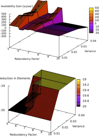
Fig. 7. Availability gain compared to proportional distribution of 30 erasure code elements with corresponding reduction in used erasure code elements for 10 nodes with mean availability of 0.75, and different variances
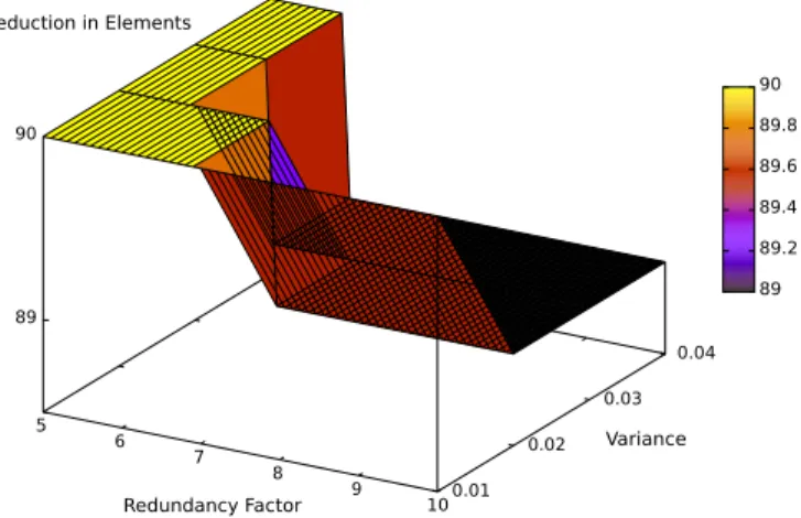
be interesting to see a comparison to our algorithm when using a normal distribution instead, as the original design goal besides a reduction in required erasure code elements was to perform well with near homogeneous node availabilities. The beta-distribution is used to simulate exceptions which diverge greatly from the average values. Since these exceptions are hard to predict, a normal distribution would be a suitable alternative. Fig. 9 shows the element reduction potential when using a normal distribution, compared to Fig. 7 which assumes a beta distribution of availability incidents.
Viewed critically, availability guarantees in cloud provider SLAs are insignificant in certain use cases, like a backup scenario, where data is rarely accessed. A short failure period of ten minutes every day would in the worst case delay a multi-hour backup process by about ten minutes. Similarly, when restoring the complete backup for data recovery, a multi-hour download process would only be delayed for a short time. In this case, statistics like mean and maximum periods of unavail-ability are meaningful. Further, SLA guarantees are only an indication of the actual availability. First, an SLA can define availability differently to our definition. Second, the guarantee only states what happens in the case of a certain guarantee violation. Data durability would be an interesting statistical metric, but giving good estimates seems hard when we need
5 6 7 8 9 10 Skype (0.544,0.105) -70000 -60000 -50000 -40000 -30000 -20000 -100000 10000 Redundancy Factor Availability Gain [s/year]
-70000 -60000 -50000 -40000 -30000 -20000 -10000 0 10000 5 6 7 8 9 10 Planetlab (0.816,0.063) Microsoft (0.738,0.061) -400 -300 -200 -100 0 100 200 300 Redundancy Factor Availability Gain [s/year]
-400 -300 -200 -100 0 100 200 300 5 6 7 8 9 10 Skype (0.544,0.105) Planetlab (0.816,0.063) Microsoft (0.738,0.061) -20 -19 -18 -17 -16 -15 Redundancy Factor Reduction in Elements -20 -19 -18 -17 -16 -15
Fig. 8. Availability gain compared to proportional distribution of 30 erasure code elements with corresponding reduction in used erasure code elements for 10 nodes with mean availabilities and variances from actual availability traces
to consider factors like economic lifetime, catastrophes and attacks on the provider’s infrastructure over a decade or more. In this case, a diversification strategy seems optimal to guard against data loss of a single provider by storing enough data to other providers to be able to recover from data loss. The multi-purpose optimisation shows that NubiSave can offer a good solution for a variety of user profiles, including those for free storage, high durability, high performance, and free
5 6 7 8 9 100.01 0.02 0.03 0.04 89 90 Redundancy Factor Variance Reduction in Elements 89 89.2 89.4 89.6 89.8 90
Fig. 9. Reduction in used erasure code elements for 10 nodes with mean availability of 0.75, assuming a normal distribution
read access. Additionally, when combined with an encryption module, these profiles can also offer security.
NubiSave retrieves data from the providers through a trans-port layer. Implementations of this layer improve the availabil-ity of data by using caches and sophisticated error handling, but they might also impair availability by bugs in the program code. The model disregards these influences which might be incorporated into NubiSave once ample statistics about the component reliability are collected. The values for availability are estimations and should be refined by empirical results for accuracy. The data availability presented by NubiSave is the minimal availability of a single data chunk according to the current configuration. Instead, a mean value for availability may be used, but the model merely considers the parallel use of storage services, by which any set of a number of elements can equally be used in reconstructing the original data, and the dis-tribution of the elements does not alter over time. In this case, the minimal availability equals the average availability. Other erasure codes depend on certain combinations of elements when decoding data. Also, the round-robin strategy, which alternates between a set of storage targets of the same size for load distribution, is another strategy implemented in NubiSave. Its mean availability that can differ greatly from its minimal availability. For simplicity, the model does not consider the latter two cases. Another simplification is that data availability refers to a single small chunk of data, even though a large file consists of several chunks. Logically, due to different transfer times, it is more probable to successfully retrieve a small chunk than a sequence of chunks, since storage nodes are more likely to fail over an increased period of transfer time. Problematically, there are few comprehensive studies on the availability of cloud storage services. For the same reason, durability, which means long term availability of data, has found little consideration as a quality parameter in the thesis. Long term studies would need to factor in large scale disaster like storms or floods, war, economic crisis or more general economic change, especially in the cloud provider domain, and finally technical change, which can lead to incompatibility for
devices and data formats.
V. CONCLUSION
PICav is a novel scheme to precisely and quickly calculate the overall availability and data distribution in heterogeneous cloud storage environments with minimal fragment size and transmission overhead. We have shown that, on average, PICav compares well against related work. By extending NubiSave, we have successfully realised PICav in an existing cloud storage controller and verified its usefulness from the practical perspective. Future research will concentrate on fragment dis-tribution decisions under additional constraints such as privacy and computability.
ACKNOWLEDGEMENTS
This work has been partially funded by the German Re-search Foundation (DFG) under project agreements SCHI 402/11-1.
REFERENCES
[1] H. Abu-Libdeh, L. Princehouse, and H. Weatherspoon, “RACS: A Case for Cloud Storage Diversity,” in1st ACM Symposium on Cloud Computing (SoCC), Indianapolis, Indiana, USA, June 2010, pp. 229– 240.
[2] J. Spillner, J. Müller, and A. Schill, “Creating Optimal Cloud Storage Systems,” Future Generation Computer Systems, vol. 29, no. 4, pp. 1062–1072, June 2013, dOI: http://dx.doi.org/10.1016/j.future.2012.06.004.
[3] V. Abhishek, I. A. Kash, and P. Key, “Fixed and Market Pricing for Cloud Services,” in 7th Workshop on the Economics of Networks, Systems, and Computation (NetEcon), Orlando, Florida, USA, March 2012, pp. 7–12.
[4] C. Cérin, C. Coti, P. Delort, F. Diaz, M. Gagnaire, Q. Gaumer, N. Guil-laume, J. L. Lous, S. Lubiarz, J.-L. Raffaelli, K. Shiozaki, H. Schauer, J.-P. Smets, L. Séguin, and A. Ville, “Downtime statistics of current cloud solutions,” International Working Group on Cloud Computing Resiliency, June 2013.
[5] L. Pamies-Juarez, P. García-López, M. Sánchez-Artigas, and B. Herrera, “Towards the design of optimal data redundancy schemes for heteroge-neous cloud storage infrastructures,”Comput. Netw., vol. 55, no. 5, pp. 1100–1113, April 2011.
[6] J. S. Plank, J. Luo, C. D. Schuman, L. Xu, and Z. Wilcox-O’Hearn, “A Performance Evaluation and Examination of Open-Source Erasure Coding Libraries For Storage,” in7th USENIX Conference on File and Storage Technologies (FAST), February 2009, pp. 253–266.
[7] D. Ford, F. Labelle, F. I. Popovici, M. Stokely, V.-A. Truong, L. Barroso, C. Grimes, , and S. Quinlan, “Availability in Globally Distributed Storage Systems,” in9th USENIX Symposium on Operating Systems De-sign and Implementation (OSDI), Vancouver, British Columbia, Canada, October 2010, pp. 61–74.
[8] O. Khan, R. Burns, J. S. Plank, W. Pierce, and C. Huang, “Rethinking Erasure Codes for Cloud File Systems: Minimizing I/O for Recovery and Degraded Reads,” in10th USENIX Conference on File and Storage Technologies (FAST), San Jose, California, USA, February 2012. [9] M. Sathiamoorthy, M. Asteris, D. Papailiopoulos, A. G. Dimakis,
R. Vadali, S. Chen, and D. Borthakur, “XORing Elephants: Novel Erasure Codes for Big Data,” The 39th International Conference on Very Large Data Bases (VLDB), vol. 6, no. 5, pp. 325–336, August 2013.
[10] A. K. Gupta and S. Nadarajah,Handbook of Beta Distribution and Its Applications. Dekker, 2004, p. 362.
[11] L. Pamies-Juarez, P. García-López, and M. Sánchez-Artigas, “Heterogeneity-Aware Erasure Codes for Peer-to-Peer Storage Systems,” in Proceedings of the 38th International Conference on Parallel Processing (ICPP), Vienna, Austria, September 2009, pp. 412–419.