Designing multi-label classifiers
that maximize
F
measures: state of the art
Ignazio Pillai, Giorgio Fumera, Fabio Roli Dept. of Electrical and Electronic Eng., University of Cagliari
Piazza d’Armi, 09123 Cagliari, Italy Email addresses: {pillai,fumera,[email protected]}
URL: http://pralab.diee.unica.it
Abstract
Multi-label classification problems usually occur in tasks related to informa-tion retrieval, like text and image annotainforma-tion, and are receiving increasing at-tention from the machine learning and pattern recognition fields. One of the main issues under investigation is the development of classification algorithms capable of maximizing specific accuracy measures based on precision and re-call. We focus on the widely used F measure, defined for binary, single-label problems as the weighted harmonic mean of precision and recall, and later ex-tended to multi-label problems in three ways: macro-averaged, micro-averaged and instance-wise. In this paper we give a comprehensive survey of theoreti-cal results and algorithms aimed at maximizingF measures. We subdivide it according to the two main existing approaches: empirical utility maximization, and decision-theoretic. Under the former approach, we also derive the opti-mal (Bayes) classifier at the population level for the instance-wise and micro-averagedF, extending recent results about the single-labelF. In a companion paper we shall focus on the micro-averaged F measure, for which relatively fewer solutions exist, and shall develop novel maximization algorithms under both approaches.
Keywords: multi-label classification,F measure, learning algorithms, empirical utility maximization, decision-theoretic approach
1. Introduction
Multi-label (M-L) classification problems, like document categorization, and image and video annotation, usually occur in the design of information retrieval (IR) systems. They consist of deciding whether an instance (e.g., a document) is relevant or not to a given set of queries, which can be viewed as non-mutually exclusive labels. An instance can thus be assigned more than one label. Over the past ten years, M-L classification problems have received an increasing attention from the pattern recognition and machine learning research communities (see, e.g., [33, 36]). One of the main topics under investigation is the development of learning algorithms tailored to specific M-L accuracy measures. Such measures are mostly based on precision and recall, which are the main metrics used for evaluating the performance of IR systems. They are different from the ones used in single-label (S-L) problems, like the misclassification probability.
In this work we focus on the widely usedF measure. It has been originally proposed to evaluate IR systems in [30, 34], and is defined as the weighted harmonic mean of precision and recall. It is also used to evaluate the accuracy of S-L binary classifiers aimed at discriminating instances relevant to a query from non-relevant ones.1
Three different versions of theFmeasure have subsequently been defined for M-L problems: instance-wise, macro- and micro-averaged. Under the viewpoint of the target accuracy measure, the existing approaches to M-L classifier design can be subdivided into two groups. Works in the first group (including most of the earlier ones) do not focus on a specific measure; they use S-L learning algo-rithms, and deal with multiple labels per sample usingproblem transformation
oralgorithm adaptation strategies (see the surveys of [33, 36]). Among the for-mer, the simplest one isbinary relevance(BR), which consists of independently
1The S-LF measure is also used in binary problems not related to IR, but characterized
by relevant class imbalance. In this case the misclassification probability is not a suitable performance measure, since a classifier that always predicts the majority class attains an accuracy equal to the corresponding prior.
learning a binary classifier for each label, disregarding label correlation; other approaches have been proposed to attain a trade-off between taking into ac-count label dependencies and keeping computational complexity low. Works in the second group focus on developing algorithms to maximize a specific accuracy measure, most often one of the M-LF measures. Maximizing theF measures (including the L one) is however particularly difficult since, contrary to S-L measures like accuracy, they do not decompose either over samples, or over labels, or both. Two different approaches for maximizing the S-L and M-L F measures have been considered, in turn [19]. The empirical utility maximization (EUM) approach aims at finding the decision rule which maximizes the chosen F measure on a finite sample oflabelled instances; this approach has been used to develop several learning algorithms. The decision-theoretic approach (DTA) aims instead at finding the label assignments that maximize the expected value of the chosenF measure on a fixed set of unlabeled instances, with respect to their joint label-conditional probability; in practice, this probability is estimated from training data, whereas the unlabeled instances correspond to testing data. In the present paper we give a comprehensive survey of existing algorithms for maximizing theF measures, which is still lacking in the literature. Nearly all works published in pattern recognition venues follow the EUM approach. Both EUM and DTA have been considered in machine learning venues, instead, where different EUM algorithms have been proposed, and the optimal (Bayes) classifier at the population level has also been recently derived for some of the F measures. Moreover, most of the earlier works focused on a single version of theF measure, and only recently (since [5]) the distinction between the S-L and M-LF, and between the three M-L versions, was clearly pointed out. Our survey can be useful for further developments in this field, especially for the pattern recognition community. As a by-product, we also derive the optimal classifier at the population level for the M-L instance-wise and micro-averaged F, under the EUM approach, extending recent results about the S-L F.
In a companion paper [28] we shall focus on the M-L micro-averagedF, for which relatively fewer solutions exist, and shall develop both learning algorithms
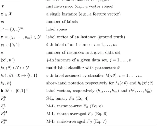
Table 1: Notation used in this paper.
X instance space (e.g., a vector space)
x∈ X a single instance (e.g., a feature vector)
m number of labels
Y={0,1}m
label space
y={y1, . . . , ym} ∈ Y label vector of an instance (ground truth)
yi∈ {0,1} i-th label of an instance,i= 1, . . . , m
n number of instances in a given data set
(xj,yj) j-th instance of a given data set,j= 1, . . . , n
h(·;θ) :X 7→ Y multi-label classifier with parametersθ
hi(·;θ) :X 7→ {0,1} i-th label assigned by classifierh(·;θ),i= 1, . . . , m
hi,hji short-hand notation respectively forhi(·;θ) andhi(xj;θ)
h,hj∈ {0,1}m
label vectors, respectively (h1, . . . , hm) and (hj1, . . . , h
j m) Fβb S-L, binaryFβ (Eq. 4) Fi β M-L, instance-wiseFβ (Eq. 5) FβM M-L, macro-averagedFβ (Eq. 6) Fβm M-L, micro-averagedFβ (Eq. 7)
based on EUM and an inference algorithm based on DTA.
The rest of this paper is structured as follows. After giving a formal definition of the F measures in Sect. 2, in Sect. 3 we describe EUM and DTA. We then survey existing works based on such approaches, respectively in Sects. 4 and 5, for each of theF measures (including the S-LF).
2. Definition ofF measures
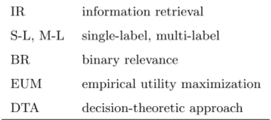
In Tables 1 and 2 we summarize respectively the notation and the abbre-viations used in this paper. We shall use upper-case letters to denote random variables, and the corresponding lower-case letters to denote their values.
For a given M-L problem, let mdenote the number of labels, X the input space (e.g., a feature vector space),x∈ X an instance (e.g., a feature vector), and y∈ Y = {0,1}m the corresponding label vector, wherey
Table 2: List of the abbreviations used in this paper.
IR information retrieval
S-L, M-L single-label, multi-label
BR binary relevance
EUM empirical utility maximization DTA decision-theoretic approach
thatxis (not) relevant to thei-th label. A M-L classifier is commonly formalized as a function
h(x;θ) = (h1(x;θ), . . . , hm(x;θ))∈ Y, (1)
where hi(x;θ) = 1 (0) means that x is deemed as (non-)relevant to the i-th
label, andθ denotes the parameter vector to be set by the learning algorithm. Precision (p) and recall (r) are the main measures used for evaluating the quality of the results produced by IR systems, in terms of the “degree of matching” between the true and the estimated relevance to a given query. They are defined respectively as the probability that a retrieved instance (e.g., a document) is relevant, and as the probability of retrieving a relevant instance, which are complementary aspects of an IR system’s performance. LetS={(xj, yj)}n
j=1be a set of instances, whereyj∈ {0,1}denotes the relevance ofxjto the considered
query, and let hj ∈ {0,1} denote the estimated relevance. Let T P, F P and
F Ndenote the corresponding number oftrue positive(whenhj =yj = 1),false positive(hj= 1,yj= 0) andfalse negative(hj= 0,yj= 1) decisions. Precision and recall can be estimated on the finite sampleS as:
p= T PT P+F P = Pn j=1y jhj Pn j=1hj , (2) r= T PT P+F N = Pn j=1yjhj Pn j=1yj . (3)
Single-label, binary F measure. The F measure has been originally proposed for IR systems, to combinep andr into a scalar [30, 34]. Based on principled arguments, it is defined as the weighted harmonic mean ofpand r.
It is also often used to evaluate the accuracy of S-L, binary classifiers (m= 1) whose goal is to discriminate between relevant instances to a given query and non-relevant ones. The S-LF is defined on a finite sample as (the superscript ‘b’ stands for ‘binary’):
Fβb= 1 +β2 1 p +β 2 1 r = (1 +β 2)T P (1 +β2)T P +β2F N+F P = (1 +β2)Pn j=1y jhj β2Pn j=1yj+ Pn j=1hj , (4)
whereβ∈[0,+∞) controls the trade-off betweenpandr. Note thatFb
0 =pand Fb
+∞=r. Forβ = 1 one obtains the unweighted harmonic mean:F1b= 2 1/p+1/r. Multi-label F measures. Three different M-L versions of theF measure have been defined. Theinstance-wise F views instances as queries, whose rel-evant labels have to be retrieved. It is thus defined for asingle instance (x,y) as: Fβi = (1 +β2)Pm i=1yihi β2Pm i=1yi+P m i=1hi . (5)
Themacro-averaged F is computed on a set of instances; it is defined as the average of the S-L F measures computed for each label, and gives the same weight to each label:
FβM= m X i=1 (1 +β2)T Pi (1 +β2)T P i+β2F Ni+F Pi = m X i=1 (1 +β2)Pn j=1y j ih j i β2Pn j=1y j i + Pn j=1h j i . (6)
Themicro-averaged F is computed after pooling the labels of all instances of a given set, and gives equal weight to each labeling decision:
Fβm = Pm i=1(1 +β 2)T P i Pm i=1[(1 +β2)T Pi+β2F Ni+F Pi] = (1 +β 2)Pn j=1 Pm i=1y j ih j i β2Pn j=1 Pm i=1y j i + Pn j=1 Pm i=1h j i . (7)
To simplify the notation, from now on we will omit the subscriptβ in the symbols denoting theF measures, when it is not necessary.
Choice between the multi-label F measures. The three M-L F mea-sures evaluate different aspects of classifier performance, and thus the choice between them is application-dependent. With regard to the problem of design-ing classifiers that maximize the M-LFmeasures, quoting from [5]: “One should
carefully distinguish these versions, as algorithms optimized with a given ob-jective are usually performing sub-optimally for other (target) evaluation mea-sures.” An empirical evidence of this fact was formerly reported in [6], where it was observed that tuning the decision thresholds of a classifier to maximize FM can decrease the corresponding Fm. In particular, it is known that the differences betweenFMandFm can be large on data sets with rare labels [16]: since the F measures disregard true negatives (i.e., instance-label pairs such thatyji =hji = 0) and their magnitude is mostly determined by the number of true positives, frequent labels dominate rare ones in Fm, whereasFM is much more sensitive to rare labels. Further insights have been given in [15]: for a rare label, a perfect classifier only marginally improvesFmover a (trivial) clas-sifier that labels all instances as non-relevant; moreover, for rare labels with an “uninformative predictive model” (i.e., a classifier which outputs the same score for all instances),Fm andFMare maximized by classifying all instances respectively as non-relevant and as relevant.
Maximizing the F measures. Under the viewpoint of classifier design, maximizing the S-L and M-L F measures is more difficult than maximizing traditional S-L measures based on the 0–1 loss function and the corresponding misclassification probability, or their variants. The latter areuni-variate mea-sures, i.e., they decompose over instances. This means that the optimal label assignment to any given instance is independent of other instances. On the contrary,FM (as well as Fb) does not decompose over instances; Fi does not decompose over labels; andFmdoes not decompose over either. Therefore,FM andFm (as well asFb) aremulti-variate, which implies that the optimal label assignments to a given instance depend also on the assignments to theother in-stances on which these measures are computed. Additionally, in the case ofFm the different label assignments, even for different instances, influence each other. Accordingly, the maximization of these measures is in principle computationally demanding, or even infeasible. Moreover, it fits only batch or off-line settings; in on-line settings one should, e.g., classify the incoming samples in batches, or consider a subset of the previously processed instances when labeling an
incom-ing one [14]. Similarly, althoughFi is uni-variate, its maximization requires in principle to consider all possible 2m label assignments, which is feasible only when the number of labels is small.
3. Approaches to F measure maximization
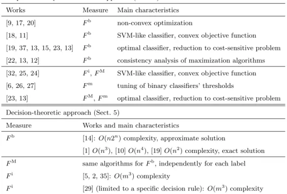
As mentioned in Sect. 1, two approaches for maximizing the F measures, both in S-L (Fb) and in M-L classification problems (Fi,FMandFm), have been proposed so far: EUM and DTA [19, 4]. The existing maximization algorithms are surveyed in the next two sections, and are summarized in Table 3. We point out that, with the only exception of [29], all works published in pattern recognition venues follow the EUM approach.
The EUM approach consists of learning a classifier of the form h(·;θ) : X 7→ Ythat maximizes the chosenFmeasure on a giventraining setof labelled instancesS={(xj,yj)}n
j=1; the learnt classifier is then used to predict the label assignments of testing data. In principle, this requires one to jointly evaluate all possible label assignments toS, which amount to 2n forFb,n×2mforFi, m×2nforFM, and 2mnforFm. Learning algorithms based on EUM have been developed for allF measures, exceptFm, and the consistency of several learning algorithms has also been investigated. In some of the most recent works, the optimal (Bayes) classifier at the population level has also been derived for the S-LF (which also applies to the M-L, macro-averagedF); it has also been shown that allF measures but the instance-wise can be maximized by reduction to a cost-sensitive problem.
The DTA (also called plug-in rule approach in [4]) focuses instead on afixed, unlabeled sample (testing data) S = {xj}n
j=1 (n = 1 in the case of F i), and predicts through an inference procedure the label assignments that maximize the expectation of the chosenF measure onS, with respect to the joint label-conditional probability distributionP(Y1, . . . ,Yn|xn, . . . ,xn). In practice, this
distribution is estimated from training data. The corresponding maximization problem is computationally very demanding as well, since the expectation has
to be be computed over all possible combinations of true and assigned labels. The number of such combinations is 22n forFb, 22m forFi,m22n forFM, and 22mn for Fm. Maximization algorithms based on DTA have been proposed so far forFb(they also apply toFM) andFi, but not forFm. The consistency of DTA has also been investigated in recent works.
EUM and DTA have been compared in [19], focusing on the S-LFb. These approaches were found to be equivalent asymptotically (i.e., for large training and test sets), provided that the underlying models are accurate. An empirical analysis also provided evidence that EUM is more robust against model mis-specification; on the other hand, if an accurate model is chosen, DTA was found to be better in the presence of rare classes, as well as in the common domain adaptation scenario whereP(X) changes whileP(Y|X) remains constant.
A comparison between EUM and DTA focused on M-L problems has later been carried out in [4], limited to the instance-wiseFi. In this comparison the EUM framework for structured loss minimization of [32] was considered, to-gether with two specific implementations based on surrogate, convex loss func-tions [25, 24] (see Sect. 4.2). The analysis of the infinite sample case showed that the DTA is consistent, i.e., it converges to the Bayes optimal classifier for the Fi measure, whereas the considered EUM algorithms are not. A fur-ther analysis on finite data sets was carried out in [4], by comparing the exact DTA-based inference algorithms for the two cases of conditionally independent and conditionally dependent labels (see Sect. 5.2), and the EUM-based learn-ing algorithms mentioned above. DTA-based algorithms were found to be more effective than EUM-based ones; they also exhibited a higher efficiency in the training step and for parameter tuning, but a lower efficiency in the inference step.
4. Empirical utility maximization approach
In this section we describe learning algorithms developed for the S-L and M-L F measures, and then summarize recent theoretical results about the EUM
Table 3: Summary of existing EUM- and DTA-based methods (described respectively in Sect. 4 and 5) for maximizing the S-LFbmeasure and the three M-LF measures.
Empirical utility maximization approach (Sect. 4)
Works Measure Main characteristics
[9, 17, 20] Fb non-convex optimization
[18, 11] Fb SVM-like classifier, convex objective function
[19, 37, 13, 15, 23, 13] Fb optimal classifier, reduction to cost-sensitive problem [22, 13, 12] Fb consistency analysis of maximization algorithms [32, 25, 24] Fi,FM SVM-like classifier, convex objective function [6, 26, 27] Fm tuning of binary classifiers’ thresholds
[23, 13] FM,Fm optimal classifier, reduction to cost-sensitive problem
Decision-theoretic approach (Sect. 5)
Measure Works and main characteristics
Fb [14]: O(n2n) complexity, approximate solution
[1]O(n3), [10]O(n4), [19]O(n2) complexity, exact solution FM same algorithms forFb, independently for each label
Fi [5, 2, 35]: O(m3) complexity
Fi [29] (limited to a specific decision rule): O(m3) complexity
approach. We finally complement such results by deriving the optimal classifier at the population level for the micro-averaged and the instance-wiseF.
Learning algorithms proposed so far can be subdivided into four categories: variants of the SVM learning algorithm (based on the maximum-margin ap-proach) [18, 11, 32, 24, 25], whose objective function is (except for [18]) a con-vex approximation of an F measure; optimization algorithms whose objective function is a non-convex approximation [9, 17, 20]; algorithms that tune the decision thresholds of binary classifiers [6, 26, 27, 22, 13, 12]; and cost-sensitive algorithms [23, 13].
4.1. Single-labelF measure
The first learning algorithm was proposed in [18], as a modification of the SVM learning algorithm. The objective function of the latter includes a penalty term which upper bounds the number of misclassified training instances. This term was was replaced by the following approximation of 2(1/F1b−1), which is a possible loss function corresponding to the use ofF1bas the accuracy measure:
Pn
j=1(1−exp(αξj))+ n+−Pnj=1I[yj = 1](1−exp(αξj))+
, (8)
whereI[a] = 1 (0) ifa=true (false),x+=x(0) ifx≥0 (<0),n+is the number of instances with label 1, andαis a positive constant. However, Eq. (8) is non-convex: finding the global minimum of the resulting objective function is not guaranteed, and the optimization problem exhibits a much higher computational complexity than the one of SVMs. Another interesting result was given in [18], related to a different, heuristic modification to the SVM penalty term, formerly proposed by other authors for balancing precision and recall. It consists of assigning different weights to misclassified instances of the two classes:
C+ n X j=1 I[yj= 1]ξj+C− n X j=1 I[yj = 0]ξj , (9)
where ξj is the hinge loss for the j-th training instance. The solution of the
corresponding learning problem turned out to approximate the one obtained using (8), for suitable values ofC+andC−. In Sect. 4.3 we shall see that recent theoretical results have proven the equivalence between maximizingFb at the population level and minimizing the expected error with suitable asymmetric misclassification costs.
In [11] an extension of the SVM learning algorithm to performance measures that do not decompose into expectations over instances, includingFb, was pro-posed. It minimizes aconvex upper bound of the corresponding loss function, and uses a multi-variate decision function which jointly labels all training in-stances (the class labels are conveniently denoted here as−1 and +1):
h(x1, . . . ,xn;w) = arg max h1,...,hn∈{−1,+1}n * w, n X j=1 hjxj + , (10)
whereh·,·idenotes the dot product. The learning problem is: minw,ξ≥0 12kwk2+Cξ s.t. ∀(h1, . . . , hn)∈ {−1,+1}n\ {(y1, . . . , yn)}: D w,Pn j=1y jxj−Pn j=1h jxjE≥∆(h1, . . . , hn, y1, . . . , yn)−ξ (11) where ∆ denotes the loss function. If the performance measure is Fb, then ∆ = 1−Fb. In principle, Eq. (10) requires one to evaluate 2n different la-bel assignments; moreover, the learning problem (11) has 2n−1 constraints. Nevertheless, since (10) is a linear function, its maximum can be computed by independently considering each of the n assignments (h1, . . . , hn). Moreover,
problem (11) can be solved with O(n2) computational complexity, thanks to the properties of Fb, using an optimization strategy proposed in [31]. SVMs turns out to be a particular case of the above classifier, when the error rate is used in (11) as the loss function.
In [9] and [17] learning algorithms that maximize continuous but non-convex approximations ofFbwere proposed, using numerical optimization techniques. In [9] the linear discriminant function of logistic regression classifiers was used, andFb is approximated similarly to Eq. (8). To deal with non-convexity, the optimization algorithm was run several times, starting from randomly chosen parameter values. In [17] the class-conditional distributionP(X|Y) is first esti-mated, then the TP, FP and FN counts are approxiesti-mated, for a given discrimi-nant function, by integratingP(X|Y) in the corresponding decision regions. The parameters of the discriminant function that maximizeFbare finally estimated by an optimization algorithm.
4.2. Multi-labelF measures
In the following we review existing EUM-based learning algorithms, sepa-rately for each of the three M-LF measures.
4.2.1. Instance-wiseF
In [32] a SVM-like classifier was proposed for structured-output problems with instance-wise performance measures, includingFi. The proposed discrimi-nant function exploits the structure and dependencies within the output values:
h(x;w) = arg max
h∈Yhw,Ψ(x,h)i, (12) where Ψ(x,h) is a feature mapping (a combined feature representation of inputs and outputs), andhw,Ψ(x,h)imeasures how “compatible” a pair (x,h) is. The learning problem is:
minw,ξ 12kwk2+n1CP n j=1ξj s.t. ∀h∈ Y \yj, j= 1, . . . , n: w, Ψ(x,yj)−Ψ(x,h) ≥∆(yj,h)−ξ j, ξj ≥0. (13)
When the performance measure isFi, then ∆ = 1−Fi. An efficient optimization algorithm was also developed, that explicitly examines only a small subset of the constraints in (13), which aren×(2m−1) in the case ofFi.2
A similar approach was proposed in [25], which explicitly models the depen-dencies (only the positive correlations) between pairs of labels. The decision function is defined as:
h(x;θ) = arg max
h∈Yh
>Ah, (14)
whereAis anm×mupper-triangular matrix defined asAii=hx, θii, andAik=
Cikθik,i6=k; the parameter vectorθiweighs the features for thei-th class;Cij
is the normalized counts of co-occurrence of labelsiandjin training instances; andθikis a scalar parameter which is forced to be non-negative, implying that
Aik>0 fori6=k, which allows (14) to be efficiently solved. The parameterθin
the left-hand side of (14) is defined as (θ1, . . . , θm, θ1,2, θ1,3, . . . , θm−1,m). The
learning problem and the proposed optimization strategy are similar respectively
2An alternative formulation was also proposed, in which the right-hand side of each
con-straint is 1−ξj/∆(y,h), as well as equivalent formulations in which quadratic termsξ2j are
to (13) and to the one of [32], to efficiently handle the constraints: minθ,ξ λ2kθk2+1nP n j=1ξj s.t. ∀h∈ Y \yj, j= 1, . . . , n: (yj)>Ayj−h>Ah≥∆(y,h)−ξ j, ξj≥0 . (15)
Finally, the specific setting in which an ensemble of independently trained binary classifiers are used for each label, and their scores are linearly combined, was considered in [8]. A non-convex approximation of Fi was devised, and an algorithm for maximizing it with respect to the combination weights was developed. We shall describe it in Sect. 4.2.3, since it was applied also toFm.
4.2.2. Macro-averagedF
In [24] a SVM-like approach similar to the one of [32] was proposed for M-L loss functions that decompose over labels, including FM. The classifica-tion problem is formulated as a reverse prediction: given a set of instances {(xj,yj)}n
j=1, themlabels are considered as the set ofinputs, and the instances that are relevant to a label are considered as the correspondingoutput. The in-put value corresponding to thei-th label is encoded as anm-dimensional vector
ai∈ {0,1}m, withai
i = 1, anda i
k = 0 fork6=i; the corresponding output values
are encoded asbi∈ {0,1}n, withbi
j = 1 (0) if thej-th instance is (not) relevant
to thei-th label. A given data set is then transformed into a set ofminstances {(ai,bi)}m
i=1made up of all possible input values and the corresponding output vectors. The decision function for thei-th label is defined as:
bi= arg max b∈{0,1}nhφ(a i,b), θi, (16) where φ(ai,b) = n X j=1 bj(xj⊗ai)∈Rd×m , (17)
dis the dimensionality of X, andθ ∈ Rd×m is a parameter matrix. Similarly
to [25], the learning problem is: minθ,ξ λ2kθk2+m1 P m i=1ξi s.t. ∀b∈ {0,1}n\bi, i= 1, . . . , m: hφ(ai,bi), θi − hφ(ai,b), θi ≥∆(bi,b)−ξ i, ξi≥0, (18)
where the loss function is defined as ∆(bi,b) = 1−Fc,i. The term m1 Pm
i=1ξi
in the objective function is a convex upper bound on ∆. An efficient, O(n2) optimization algorithm was developed for solving problem (18). It was also shown that the decision function (16) can be computed inO(n) time.
Since the M-L FM measure is the average of the corresponding S-L Fb measures, it is pertinent to investigate the relationship between the maximum-margin approach of [24] (described above) and the one formerly developed in [11] (Sect. 4.1), aimed at maximizing respectively FM and Fb. No comparison between these approaches was reported in [24]. As a contribution of this paper, here we show that these approaches are equivalent, as stated in the following Proposition:
Proposition 1. For C = 4λm1 , the M-L decision function (16) obtained by solving the learning problem (18)of [24] coincides with the set of decision func-tions (10)of independently trained binary classifiers (i.e., using BR) obtained by solving the learning problem (11)of [11].
Proof. We first prove that their decision functions are equivalent. Since ai
in [24] is defined as anm-dimensional column vector in which thei-th element is 1 and all the other ones equal 0, it follows thatxj⊗ai in Eq. (17) is ad×m matrix in which thei-th column equalsxj, and all the other elements are zero. Therefore, alsoφ(ai,b) in Eq. (17) is ad×mmatrix, in which thei-th column equalsPn
j=1bjx
j and all the other elements are zero. The argument of the arg
max in (16) can thus be rewritten as:
hφ(ai,b), θi= * n X j=1 bjxj, θi + . (19)
This means that the assignment for thei-th label depends only onθi. We can
thus rewrite the decision function (16) for thei-th label as:
bi= arg max b∈{0,1}n * n X j=1 bjxj, θi + . (20)
We now make the following change of variables:
hji = 2bij−1, hj = 2bj−1, wi =
1
Note that this implies thathj ∈ {−1,+1}. The decision function (20) for the i-th label can be rewritten as:
h1i, . . . , hni = arg maxh1,...,hn∈{−1,1}n D Pn j=1 hj+1 2 xj,2wiE = arg maxhPn j=1h jxj,w ii+hP n j=1x j,w ii . (22)
The last termhPn
j=1x
j,wiiis constant with respect toh1, . . . , hn, which makes
the decision function (22) identical to (10).
We now prove that the learning problems are equivalent, for a proper choice of their parametersλ and C. The objective function of problem (18) can be rewritten by explicitly indicating the Frobenius norm of the parameter matrix θas a function of the 2-norm of its columns, denoted asθi,i= 1, . . . , m:
min θ,ξ λ 2 m X i=1 kθik2+ 1 m m X i=1 ξi . (23)
Using (19), the constraints of (18) can be rewritten as:
∀b∈ {0,1}n\bi, i= 1, . . . , m: D Pn j=1b i jxj− Pn j=1bjxj , θi E ≥(1−Fβc,i)−ξi, ξi≥0 . (24)
It is now evident that minimizing (23) under constraints (24) amounts to solving the followingm independent optimization problems, one for each label:
minθi,ξi≥0 λ 2kθik 2+ 1 mξi s.t. ∀b∈ {0,1}n\bi: D Pn j=1b i jxj− Pn j=1bjxj , θi E ≥(1−Fβc,i)−ξi . (25)
We now make another change of variables:
yij= 2bij−1 . (26)
Together with (21), this allows us to rewrite the constraints of (25) as:
∀(h1, . . . , hj)∈ {−1,1}n\ {(y1 i, . . . , y n i)}: D Pn j=1 yj i+1 2 − hj+1 2 xj,2wiE≥(1−Fβc,i)−ξi ≡ DPn j=1(y j i −hj)xj ,wiE≥(1−Fβc,i)−ξi , (27)
which are identical to the constraints of (11), for the i-th label. Finally, us-ing (21), the objective function of (25) becomes:
λ 2k2wik 2+ 1 mξi = 1 2(4λ)kwik 2+ 1 mξi . (28)
The solution of the corresponding learning problem does not change by rescal-ing the objective function (28); dividrescal-ing it by 4λ, it becomes identical to the objective function of (11) whenC= 4λm1 , which completes our proof.
4.2.3. Micro-averagedF
Fm is the most challenging measure, since it does not decompose over in-stances nor over labels. Existing EUM-based approaches consist of using a M-L decision function defined ashi(x) = sign[fi(x)−θi], i= 1, . . . , m, wherefi(x)
are real-valued discriminant functions obtained by independently training one binary classifier for each label (using any performance measure), whereasθi∈R
are decision thresholds that are tuned afterwards (i.e., keeping fixed thefi(·)’s)
to maximize Fm on validation data.3 Let Fm(θ1, . . . , θm;S) denote the value
ofFm computed on a given data setS (e.g., a validation set) as a function of the decision thresholds. The optimal threshold values are the solution of the following optimization problem:
θ∗1, . . . , θm∗ = arg max θ1,...,θm
Fm(θ1, . . . , θm;S). (29)
This approach was first proposed in [6], where a heuristic optimization pro-cedure shown as Algorithm 1 was developed. Algorithm 1 consists of iteratively updating asingle threshold at each step by maximizing the correspondingFm, while keeping all the other thresholds at their current values, until some stop-ping criterion is met. SinceFm(θ
1, . . . , θm;S) can attain up to|S|+ 1 distinct
values with respect to any single threshold, the corresponding maximization
3Recently, it has been shown that the optimal solution can also be obtained by solving a
cost-sensitive problem with respect to the 2merror countsF PiandF Ni(see Eq. 7) [23], but
no algorithm has been developed so far to implement it. This approach will be described in Sect. 4.3.
Algorithm 1Fm maximization algorithm of [6].
Input: mtrained binary classifiersfi, a data setS, a constant >0
Output: mdecision thresholds θ(0)1 ←0, . . . , θ (0) m ←0, F(0)←Fm(θ(0)1 , . . . , θ (0) m;S), t←1 repeat fori= 1, . . . , mdo θ(it)←arg maxθFm(θ (t) 1 , . . . , θ (t) i−1, θ, θ (t−1) i+1 , . . . , θ (t−1) m ;S) end for F(t)←Fm(θ(1t), . . . , θ (t) m;S) until F(t)−F(t−1) F(0) < return θ1(t), . . . , θ (t) m
step (the arg max step of Algorithm 1) can be solved by a simple line search with complexityO(|S|). This approach was proposed in [6] without theoretical support nor optimality guarantees.
In [26, 27] we analyzed the optimization problem (29), by studying the be-havior ofFm as a function ofθ1, . . . , θm on a given sampleS. Our main result
was the following proposition (reported in [27] as Property 1):
Proposition 2. Consider any given valueθ0
1, . . . , θ0mof the decision thresholds, and the corresponding valueFm(θ0
1, . . . , θ0m;S). If no higher value ofFmcan be attained by changing any singlethreshold, while keeping all the otherm−1ones at their current value, thenFm(θ0
1, . . . , θ0m;S) = maxθ1,...,θmF m(θ
1, . . . , θm;S).
Proposition 2 allows theexact solution of (29) to be found with low computa-tional complexity. Indeed, it implies that the global maximum of Fm can be attained by starting from any threshold values, and iteratively updating one threshold at a time to any value that increases Fm (if any), until no further increase ofFm can be achieved. As a by-product, Algorithm 1 of [6] turns out to be one possible implementation of our optimization strategy above, provided that no early stopping condition is used, i.e., if the repeat-until loop ends only whenF(t)=F(t−1). We also proved that, if each threshold is initially set to−∞,4 then the exact solution of (29) is attained by considering at each step
4In practice, ifθ(0)
(e.g., in the arg max step of Algorithm 1) onlyhigher values of each threshold than the current one [27]; this reduces the computational complexity to no more thanO(m2n2).
For the sake of completeness, we finally mention a similar approach that was considered in [8] (we mentioned it also in Sect. 4.2.1). It consists of indepen-dently learning an ensemble ofK binary classifiers which output a real-valued score for each label, fi,k : X 7→ R, i = 1, . . . , m, k = 1, . . . , K. These
classi-fiers are then linearly combined: fi(x) =PKk=1wkfi,k(x) +w0. In [8],Fmwas
maximized with respect to the combination weights, that do not depend on the label. To this aim, a non-convex approximation of all three M-LF measures was defined, by approximating the TP, FP and FN counts, on a given data set, using a logistic function of the scoresfi; a quasi-Newton optimization algorithm
was then used.
4.3. Recent theoretical results about the single-labelF measure
During the past two years several works have theoretically investigated theF measure maximization problem under the EUM approach, and have derived the optimal (Bayes) solution for the S-LFb, either on a finite sample or at the pop-ulation level. Novel maximization algorithms have also been developed, some of them based on the above mentioned theoretical results, and their consistency has been analyzed.
The optimal classifier at the population level has been derived in [19, 37, 13, 15]. The corresponding expression ofFb can be obtained by replacing the TP, FP and FN counts in (4) with the corresponding probabilities, denoted astp, f pandf n, and given by:
tp=P(h(X) = 1, Y = 1) = P(Y = 1) Z x:h(x)=1 p(x|Y = 1)dx (30) f p=P(h(X) = 1, Y = 0) = P(Y = 0) Z x:h(x)=1 p(x|Y = 0)dx (31) f n=P(h(X) = 0, Y = 1) = P(Y = 1) Z x:h(x)=0 p(x|Y = 1)dx (32)
Accordingly, Fb
β =
(1+β2)tp
(1+β2)tp+β2f n+f p. The optimal classifier h∗ consists of
thresholding the posterior probability:
h∗(x) = 1, if P(Y = 1|x)≥θ∗ 0, otherwise (33) where θ∗ = F c∗ β 1+β2, and F c∗
β is the maximum S-L F. Since F
c∗
β is unknown
in practice, alsoθ∗ is unknown. Note also that θ∗ is a population-dependent value, i.e., the optimal decision whether labeling any instance as relevant or non-relevant depends not only on that instance, but also on all the other instances on whichFbis computed, as already pointed out in Sect. 2.5 Actually, this is another way to express the fact thatFb does not decompose over instances.
In practice, in the above mentioned works the optimal decision function (33) was approximated by first estimating the posteriorP(Y = 1|x), and then tuning
the decision threshold on validation data. The results in [7] allow to approximate it using a different procedure based on the ROC curve of an underlying binary classifier. It amounts to thresholding P(YF=1c∗|x)
β at 1
1+β2, where the calibrated
estimate ofP(Y = 1|x) and the estimate ofFc∗
β can be obtained from the ROC
convex hull; in this case, the threshold depends only onβ.6
Note that all the above results also apply toFM, whose optimal classifier is obtained by independently using (33) for each label; in this case, the optimal threshold can be different for each label.
An alternative solution was obtained in [23]: it was shown that the optimal classifier, both at the population level or on a finite sample, can be obtained by reduction to a cost-sensitive problem. Such a problem consists of minimizing the expected weighted error given by a linear combination of the f p and f n probabilities of each label (or the corresponding FP and FN counts), for suitable costs. Analogously to rule (33), such costs depend on the maximum Fb, and thus are unknown in practice. This implies that the optimal solution can be
5In [14] it had been already shown that the rule sign[
P(Y = 1|x)−θ], whereθis anyfixed threshold value, can not be optimal.
obtained by wrapping a cost-sensitive classification algorithm in an inner loop by an outer loop that sets the appropriate costs [23]. Although this requires in principle to solve an infinite series of cost-sensitive problems, it was shown that the cost space can be discretized to approximate the optimal solution with a desired accuracy level, by choosing the costs that provide the maximumFb value a posteriori. Interestingly, similar results were derived in [23] for the M-L FM andFm.
We finally summarize recent results about algorithms for maximizing Fb (and thus also the M-LFM).
The theoretical result of [23] mentioned above was applied in the same work to existing cost-sensitive algorithms for binary problems. Interestingly, their results apply also to the M-LFm; however, exploiting them to develop specific cost-sensitive algorithms for this measure is not straightforward, since the FP and FN counts of each class aresimultaneously involved, and was left in [23] as a future work.
In [22, 13] the consistency of “plug-in” algorithms for maximizingFb, con-sisting of thresholding an estimate of the posteriorP(Y = 1|x), and of empiri-cally computing the threshold value, was investigated. In [13] a different two-step approach was also considered (“Weighted Empirical Risk Minimization”), based on a theoretical result analogous to the one of [23]. In the first step a classifier with real-valued predictionsf(x) is learnt by minimizing a surrogate weighted loss with label-dependent costs, defined as
`(f(x), y) = (1−δ)I[y= 1]`(f(x),1) +δI[y= 0]`(f(x),0), (34)
which is known to be consistent with the (ideal) classifier given by sign (P[Y = 1|X]−δ). In the second step the empirical Fb is maximized with respect to δ. This al-gorithm is computationally less demanding than the one of [23], since it only requires a single loop to scan the values ofδ.
In [12] a similar two-step approach as the above Weighted Empirical Risk Minimization was investigated. Different possible surrogate loss functions were considered to learn the classifier at the first step, among strongly proper
com-posite loss functions, such as logistic, squared-error, and exponential loss. The results provided in [12] are not limited to the consistency of the considered ap-proach, as in [13], but are valid also for finite samples; in particular, it was shown that the regret of the considered classifier, measured with respect to the target metric, is upper bounded by the regret of the score functionf(·) measured with respect to the surrogate loss.
A different algorithm was developed in [20], based on point-based stochastic updates, and in particular on stochastic alternate maximization. For the sake of completeness we also mention that in [21] some algorithms were developed for maximizing versions of the macro- and micro-averagedF defined for multi-class S-L problems, which are different from the M-L versions considered in this paper. In particular, we point out that if the micro-averagedF of Eq. (7) (which is different from the one considered in [21]) is used in a multi-class S-L problem, it reduces to classification accuracy [16].
Finally, it is worth pointing out that most of the above results apply to broad classes of performance measures based on ratios of TP, FN and FP counts, beside theF measures.
4.4. Optimal classifier for the multi-label micro-averaged and instance-wiseF Here we show that the above mentioned results of [19, 37, 13, 15] on the S-LFbcan be exploited to derive the optimal classifier at the population level, under the EUM approach, also for the the M-LFm.7 To this aim, we follow an analogous proof procedure as the one in [15]. We then derive derive also the optimal classifier forFi. As mentioned above, whereas the optimal classifier for the S-LFb, and for the M-LFM andFm, can also be obtained by reduction to cost-sensitive problems, no analogous solution is known for theFi [23].
Micro-averaged F. Our result is given by the following proposition.
Proposition 3. The optimal classifier at the population level for Fβm consists
of decidinghi(x) = 1, if and only if: P(Yi= 1|x)≥ F∗m β 1 +β2 , (35) whereF∗m
β is the optimal value ofFβm.
Proof. Assume that the optimal decisions for all labels have already been found on the whole instance spaceX, except for thek-th label in a region ∆⊂ X around a givenx∗. Now we write theFβmat the population level, by separating the contribution of the decisionhk(x) on ∆. Using Eq. (30), the term at the
numerator of the empirical Fm
β of Eq. (7) corresponding to
Pm
i=1T Pi, minus
the contribution ofhk(x) on ∆, is given by the following expression, which we
denote again astpfor the sake of simplicity:
tp = Pm i=1,i6=kP(Yi= 1) R x∈X:hi(x)=1p(x|Yi = 1)dx+ P(Yk = 1) R x∈X −∆:hk(x)=1p(x|Yk= 1)dx. (36)
The terms corresponding toPm
i=1F Pi andP m
i=1F Ni in Eq. (7) can be written
similarly, using Eqs. (31) and (32); we denote them respectively asf p andf n. To keep the following expressions simple, we also write:
bk = P(Yk= 1), P1k(∆) = R x∈∆p(x|Yk = 1)dx, P0k(∆) = R x∈∆p(x|Yk = 0)dx. (37)
The value ofFβmcan now be written by considering the two possible choices for hk(x),x∈∆. By choosinghk(x) = 1, we get: Fβ0m= (1 +β 2) [tp+b kP1k(∆)] (1 +β2) [tp+b kP1k(∆)] +β2f n+f p+ (1−bk)P0k(∆) . (38)
By choosinghk(x) = 0, instead, we get:
Fβ00m= (1 +β 2)tp (1 +β2)tp+β2[f n+β2b
kP1k(∆)] +f p
. (39)
Accordingly, the optimal decision rule for thek-th label in ∆ is hk(x) = 1, if
and only ifF0m
β ≥F
00m
β . After some algebraic manipulations, this amounts to:
bkP1k(∆) (1−bk)P0k(∆) ≥ tp β2tp+β2f n+f p+β2b2 kP12k(∆) . (40)
Let us now take the limit ∆ → {x∗}. The left-hand side of inequality (40) becomes (see also Eq. 37):
lim ∆→{x∗} bkP1k(∆) (1−bk)P0k(∆) = lim ∆→{x∗} R x∈∆P(Yk = 1|x)p(x)dx R x∈∆P(Yk = 0|x)p(x)dx =P(Yk= 1|x ∗) P(Yk= 0|x∗) . (41) Since lim∆→{x∗}P12k(∆) = 0, for the right-hand side of inequality (40) we get:
lim ∆→{x∗} tp β2tp+β2f n+f p+β2b2 kP12k(∆) = tp ∗ β2tp∗+β2f n∗+f p∗ , (42) wheretp∗ denotes the value of Eq. (36) computed in the whole instance space X (except for the zero-measure elementx), corresponding to the optimal micro-averaged F, and similarly for f n∗ and f p∗. Finally, taking into account that
P(Yk = 0|x) = 1−P(Yk= 1|x), after some algebraic manipulations on Eqs. (41)
and (42) we obtain the claimed optimal decision rule:
P(Yk = 1|x∗)≥ tp∗ (1 +β2)tp∗+β2f n∗+f p∗ = F∗m β 1 +β2 . (43)
Instance-wiseF. In this case the optimal classifier is given by the following proposition.
Proposition 4. For a given instancex, the optimal classifier at the population level forFi
βconsists of decidinghi(x) = 1for them∗ labels exhibiting the highest posteriors, and hi(x) = 0 to the remaining ones, where 0 ≤m∗ ≤ m is given by: m∗= arg max k∈{0,...,m} (1 +β2)Pk i=0P(Y(i)= 1|x) k+β2Pm i=1P(Yi= 1|x) , (44)
where we writeP(Y(0)= 1|x) = 0, andY(1), . . . , Y(m)denote the labels sorted for
decreasing values of the posteriorsP(Yi= 1|x).
Proof. Since Fi is computed on a single instance x (see Eq. 5), its prob-abilistic definition involves only the posteriors P(Yi|x). For ease of notation,
let P = {i : hi(x) = 1}, N = {i : hi(x) = 0}, Pi1 = P(Yi = 1|x), and Pi0=P(Yi= 0|x). We then have: Fβi = (1 +β 2)P i∈PPi1 (1 +β2)P P +β2P P +P P . (45)
SinceP i∈P(Pi1+Pi0) =|P|, andPi∈PPi1+Pi∈NPi1=P m i=1Pi1, we get: Fβi =(1 +β 2)P i∈PPi1 |P|+β2Pm i=1Pi1 . (46)
Note that, for any given|P|>0, Eq. (46) is maximized by decidinghi(x) = 1
for the|P| labels exhibiting the highest posteriors Pi1, and hi(x) = 0 for the
remaining labels. It immediately follows thatFβi is maximized by the decision rule claimed above.
5. Decision-theoretic approach
F measure maximization algorithms based on DTA have been proposed so far forFb and Fi. We point out that no specific algorithm for FM has been developed under this approach, since the same algorithms forFbcan be applied, independently for each label (under the usual assumption of i.i.d. instances). No algorithm based on the DTA has been developed yet forFm, instead; we shall fill this gap in our companion paper [28].
5.1. Single-labelF
The label assignment that maximizes the expected valueE[Fb
β] on a given
set of instancesx1, . . . ,xn is given by:
(h∗1, . . . , h∗n) = arg max (h1,...,hn)∈{0,1}n X y1,...,yn∈{0,1}n P(y1, . . . , yn|x1, . . . ,xn) (1 +β2)Pn j=1y jhj β2Pn j=1yj+ Pn j=1hj . (47)
If the labels are conditionally independent, i.e., P(Y1, . . . , Yn|x1, . . . ,xn) =
Qn
j=1P(Y
j|xj), then only up to n2n combinations of true and assigned labels
need to be evaluated, out of all possible 22n combinations [14]. This is because
each summand in (47) (i.e., the value ofFb
β for fixedy1, . . . , yn) is maximized by
one of thenlabel assignments in which the label 1 is given to then0≤ninstances exhibiting then0 highest posteriorsP(Yj = 1|xj), for somen0∈ {0, . . . , n}[14].
Exact inference algorithms with lower computational complexity, under the assumption of conditionally independent labels, were subsequently derived in [1],
Algorithm 2Inference algorithm for maximizingE[Fβb] for a rationalβ
2 [19] Input: pandq, whereβ2=p/q; the posteriorsp
j:=P(Yj= 1|xj), j= 1, . . . , n
Output: the valuesfβ,1, . . . , fβ,n
for 0≤j≤n, setC[j] as the coefficient ofzjin the polynomial [p1z+ (1−p1)]. . .[pnz+ (1−pn)] S[j]←q/j, j= 1, . . . ,(q+r)n forn0=nto 1do fβ;n0 ←Pn k1=0(1 + r/q)k 1C[k1]S[rk+qk1] forj= 1 to (q+r)(n0−1)do S[j]←(1−pn0)S[j] +pn0S[j+q] end for end for returnfβ,1, . . . , fβ,n
withO(n3) complexity; in [10], withO(n4) complexity; and in [19], withO(n3) complexity, which reduces toO(n2) time andO(n) space complexity whenβ2 is rational. We report this latter procedure as Algorithm 2, as it is the one with lowest computational complexity. It provides the n+ 1 values of the expected Fb
β, denoted as fβ,0, . . . , fβ,n, corresponding to assigning hj = 1 to the n0
in-stances exhibiting the highest posteriors, forn0∈ {0, . . . , n}. The optimal label assignment is the one corresponding to the highestfβ,n0.
In the most general case when the independence assumptions does not hold, one can use the exact inference algorithm developed in [5] for Fi (described in Sect. 5.2), with O(n3) complexity. This is possible because the expression of Fb (4), and thus problem (47), are formally identical respectively to the expression ofFi (see Eq. 5 and to problem 48).
5.2. Instance-wiseF
The label assignmenth∗that maximizesE[Fβi] for a given instancexis given
by: h∗= arg max h∈Y X y∈Y P(y|x) (1 +β2)Pm i=1yihi β2Pm i=1yi+P m i=1hi . (48)
This problem has the same form as (47), but in this case the assumption of con-ditionally independent labels is not realistic, and thus the inference algorithms of [14, 1, 10, 19] do not provide the exact solution. An exact solution with
Algorithm 3The inference algorithm of [5] for maximizing E[Fi] Input: the matrixP of Eq. (49) and the value ofP(Y=0|x)
Output: the label assignment of Eq. (48) compute the matrixW defined by Eq. (50) F ←P W, h(0)←0, E0←P(Y=0|x)
fork= 1 tomdo
seth(k) such thathi= 1 for the top-kelementsFi,k in thek-th column ofF,
andhi= 0 for the other elements
Ek←2Pmi=1h(ik)Fi,k
end for
q←arg maxk=0,...,mEk
return h(q)
O(m3) complexity was derived in [5, 4, 2, 35]. It does not require the knowledge of the full distributionP(Y|x), but only of them2+ 1 probabilities
P(Y=0|x)
andP(Yi= 1, SY =s|x),i, s= 1, . . . , m, where0={0}m, andsY =Pmi=1Yiis
the number of classesxis relevant to. The inference algorithm of [5] consists of two nested maximization steps,8 and is reported as Algorithm 3, whereP and W denote them×mmatrices defined as:
Pi,s=P(Yi= 1, SY =s|x), i, s= 1, . . . , m , (49)
Wi,k=
1
β2i+k, i, k= 1, . . . , m , (50) andF denotes the matrixP W. It is worth noting that, when the assumption of conditionally independent labels does not hold, the difference between the exact solution provided by Algorithm 3 and the ones provided by algorithms based on such an assumption can theoretically become arbitrarily large [5].
In [5, 2, 35], P(Y=0|x) andP are estimated by sampling from the
distri-butionP(Y|x). The latter is in turn estimated using the Probabilistic Classifier
Chains (PCC) method [3], which exploits the product rule of probability:
P(Y|x) =
m
Y
i=1
P(Yi|x, y1, . . . , yi−1), (51)
8This approach had already been proposed in [10], but their inference algorithm exhibits
and learnsmprobabilistic classifiers that independently estimate each of them terms in the right-hand side of Eq. (51). To this aim, linear regularized logis-tic regression was used in [5, 2]. In [4, 35] P(Y=0|x) andP were estimated
using a reduction approach, by independently solving the following m+ 1 S-L multi-class probability estimation problems. For a given i ∈ {1, . . . , m},
P(Yi= 1, SY|x) can be rewritten asP(Yi0|x) by defining a new random variable
Yi0 =I[Yi = 1]×SY ∈ {0, . . . , m}; then P(Yi0|x) can be estimated, e.g., using
multinomial regression. Similarly,P(Y =0|x) is obtained by a reduction to a binary problem associated to a random variableY0 =I[Y=0]∈ {0,1}, by
esti-matingP(Y0|x). On the one hand, the latter approach avoids a computationally
demanding sampling step; on the other hand, it produces non-calibrated prob-abilities; a post-processing step is thus required, or additional constraints have to be included in the above learning problems [4].
A different approach was proposed in [29], focused on the following decision rule: hi= 1, ifP(Yi= 1|x)≥θ(x) 0, otherwise i= 1, . . . , m (52)
It labels a sample as relevant to the labels whose marginal posterior exceeds a thresholdθ(x) which depends on the sample itself (equivalently, to the labels exhibiting the top-k(x) values ofP(yi|x), where the valuek(x) depends again
on the sample). A dynamic programming strategy withO(m3) complexity was proposed to find the value ofθ(x) (ork(x)) that maximizes the expectation in Eq. (48). Note however that, if the labels are not conditionally independent, the decision rule (52) is not guaranteed to provide the global maximum ofE[Fi] [14].
6. Conclusions
We provided a unifying, comprehensive survey of the existing approaches and algorithms aimed at maximizing theFmeasures in multi-label classification problems. We believe this is a useful contribution for further developments in this field, due to the increasing interest on applications related to information
retrieval, and on the corresponding measures of classification accuracy, from both the pattern recognition and machine learning research communities.
Works published over the past few years considerably improved the knowl-edge about F measures, and provided theoretically-grounded algorithms for their optimization. The optimal (Bayes) classifier at the population level is now known both for the S-L and for all three M-L F measures; in particular, the ones for the M-L micro-averaged and instance-wise F were explicitly derived in this paper. An equivalent solution based on a reduction to cost-sensitive problems is also known, except for the M-L, instance-wise F, and algorithms based on this approach have already been derived for the S-LF and the M-L, macro-averagedF. Different maximization algorithms have also been proposed for all these measures, and the consistency of some of them has been proven. Only for the M-L micro-averagedF relatively fewer solutions are available: un-der the empirical utility maximization approach, only maximization algorithms that tune the decision thresholds of binary classifiers are known, and no maxi-mization algorithm based on the decision-theoretic approach has been derived so far. We shall fill these gaps in our companion paper [28].
Acknowledgment: This work has been supported by the project CRP– 59872 funded by Regione Autonoma della Sardegna, L.R. 7/2007, Bando 2012. We thank the reviewers of a previous version of this paper for their detailed and constructive comments.
References
[1] K.M.A. Chai. Expectation of F-measures: Tractable exact computation and some empirical observations of its properties. InProc. Int. ACM SIGIR Conf. Research and Development in Inf. Retr., pages 593–594, 2005. ACM.
[2] W. Cheng, K. Dembczy´nski, E. H¨ullermeier, A. Jaroszewicz, and W. Waegeman. F-measure maximization in topical classification. InRough
Sets and Current Trends in Computing, LNCS vol. 7413, pages 439–446. Springer, 2012.
[3] K. Dembczy´nski, W. Cheng, and E. H¨ullermeier. Bayes optimal multilabel classification via probabilistic classifier chains. InProc. Int. Conf. Machine Learning, pages 279–286, 2010.
[4] K. Dembczy´nski, A. Jachnik, W. Kotlowski, W. Waegeman, and E. H¨ullermeier. Optimizing the F-measure in multi-label classifica-tion: Plug-in rule approach versus structured loss minimization. In
Proc. Int. Conf. Machine Learning, 2013.
[5] K. Dembczy´nski, W. Waegeman, W. Cheng, and E. H¨ullermeier. An Exact Algorithm for F-Measure Maximization. In Neural Inf. Proc. Systems, pages 1404–1412, 2011.
[6] R.-En Fan and C.-J. Lin. A Study on Threshold Selection for Multi-label Classification. Tech.rep., National Taiwan University, 2007.
[7] P. Flach and M. Kull. Precision-Recall-Gain Curves: PR Analysis Done Right. InNeural Inf. Proc. Systems, pages 838–846, 2015.
[8] A. Fujino, H. Isozaki, and J. Suzuki. Multi-label Text Categorization with Model Combination based on F1-score Maximization. Proc. Int. Joint Conf. Natural Language Proc., 2008.
[9] M. Jansche. Maximum expected F-measure training of logistic regression models. InProc. Int. Conf. on Human Language Technology and Empirical Methods in Natural Language Processing, pages 692–699, 2005.
[10] M. Jansche. A maximum expected utility framework for binary sequence labeling. In Proc. Annual Meeting of the Association of Computational Linguistics, pages 736–743, 2007.
[11] T. Joachims. A Support Vector Method for Multivariate Performance Mea-sures. InInt. Conf. on Machine Learning, pages 377–384, 2005.
[12] W. Kotlowski and K. Dembczy´nski. Surrogate regret bounds for generalized classification performance metrics. CoRR, abs/1504.07272, 2015.
[13] O. Koyejo, N. Natarajan, P.K. Ravikumar, and I.S. Dhillon. Consistent bi-nary classification with generalized performance metrics. InAdv. in Neural Inf. Proc. Systems 27, pages 2744–2752, 2014.
[14] D.D. Lewis. Evaluating and optimizing autonomous text classification sys-tems. In Proc. Int. ACM SIGIR Conf. Research and Development in In-formation Retrieval, pages 246–254, 1995. ACM.
[15] Z.C. Lipton, C. Elkan, and B. Narayanaswamy. Optimal thresholding of classifiers to maximize F1 measure. InProc. Machine Learning and Knowl-edge Discovery in Databases - European Conf., ECML PKDD, Part II, LNCS vol. 8725, pages 225–239. Springer, 2014.
[16] C.D. Manning, P. Raghavan, and H. Sch¨utze. Introduction to Information Retrieval. Cambridge University Press, 2008.
[17] M. Di Martino, G. Hern´andez, M. Fiori, and A. Fern´andez. A new frame-work for optimal classifier design. Patt. Rec., 46(8):2249–2255, 2013.
[18] D.R. Musicant, V. Kumar, and A. Ozgur. Optimizing F-measure with Support Vector Machines. InInt. Florida Artif. Int. Research Society Conf., pages 356–360. AAAI Press, 2003.
[19] Ye Nan, K.M.A. Chai, W.S. Lee, and H.L. Chieu. Optimizing F-measure: A tale of two approaches. InProc. Int. Conf. on Machine Learning, 2012.
[20] H. Narasimhan, P. Kar, and P. Jain. Optimizing non-decomposable per-formance measures: A tale of two classes. In Proc. Int. Conf. Machine Learning,JMLR Proceedings vol. 37, pages 199–208, 2015.
[21] H. Narasimhan, H.G. Ramaswamy, A. Saha, and S. Agarwal. Con-sistent multiclass algorithms for complex performance measures. In
Proc. Int. Conf. Machine Learning,JMLR Proceedingsvol. 37, pages 2398– 2407, 2015.
[22] H. Narasimhan, R. Vaish, and S. Agarwal. On the statistical consistency of plug-in classifiers for non-decomposable performance measures. In Adv. in Neural Inf. Proc. Systems 27, pages 1493–1501, 2014.
[23] S.P. Parambath, N. Usunier, and Y. Grandvalet. Optimizing F-measures by cost-sensitive classification. In Adv. in Neural Inf. Proc. Systems 27, pages 2123–2131, 2014.
[24] J. Petterson and T.S. Caetano. Reverse multi-label learning. InAdvances in Neural Information Processing Systems 23, pages 1912–1920, 2010.
[25] J. Petterson and T.S. Caetano. Submodular multi-label learning. InAdv. in Neural Information Processing Systems 24, pages 1512–1520, 2011.
[26] I. Pillai, G. Fumera, and F. Roli. F-Measure Optimisation in Multi-label Classifiers. InInt. Conf. Pattern Recognition, 2012.
[27] I. Pillai, G. Fumera, and F. Roli. Threshold optimisation for multi-label classifiers. Pattern Recognition, 46(7):2055–2065, 2013.
[28] I. Pillai, G. Fumera, and F. Roli. Designing multi-label classifiers that maximize the micro-averaged F measure (submitted).
[29] J.R. Quevedo, O. Luaces, and A. Bahamonde. Multilabel classifiers with a probabilistic thresholding strategy. Patt. Rec., 45(2):876–883, 2012.
[30] C.J. Van Rijsbergen. Foundation of evaluation.Journal of Documentation, 30(4):365–373, 1974.
[31] I. Tsochantaridis, T. Hofmann, T. Joachims, and Y. Altun. Support vector machine learning for interdependent and structured output spaces. InProc. Int. Conf. Machine Learning, page 104, 2004.
[32] I. Tsochantaridis, T. Joachims, T. Hofmann, and Y. Altun. Large margin methods for structured and interdependent output variables. J. Machine Learning Research, 6:1453–1484, 2005.
[33] G. Tsoumakas, I. Katakis, and I. Vlahavas. Mining multi-label data. Data Mining and Knowledge Discovery Handbook, pages 667–685, 2010.
[34] C.J. van Rijsbergen. Information Retrieval. Butterworth, 1979.
[35] W. Waegeman, K. Dembczy´nski, A. Jachnik, W. Cheng, and E. H¨ullermeier. On the Bayes-optimality of F-measure maximizers. J. Ma-chine Learning Research, 15:3333–3388, 2014.
[36] M.-L. Zhang and Z.-H. Zhou. A review on multi-label learning algorithms.
IEEE Trans. Knowledge and Data Eng., 26(8):1819–1837, 2014.
[37] M.-J. Zhao, N.U. Edakunni, A. Pocock, and G. Brown. Beyond Fano’s inequality: bounds on the optimal F-score, BER, and cost-sensitive risk and their implications.J. Mach. Learning Research, 14(1):1033–1090, 2013.