This is an Open Access document downloaded from ORCA, Cardiff University's institutional repository: http://orca.cf.ac.uk/74725/
This is the author’s version of a work that was submitted to / accepted for publication. Citation for final published version:
Artemiou, Andreas and Tian, Lipu 2015. Using sliced inverse mean difference for sufficient dimension reduction. Statistics & Probability Letters 106 , pp. 184-190. 10.1016/j.spl.2015.07.025
filefile Publishers page:
Please note:
Changes made as a result of publishing processes such as copy-editing, formatting and page numbers may not be reflected in this version. For the definitive version of this publication, please refer to the published source. You are advised to consult the publisher’s version if you wish to cite
this paper.
This version is being made available in accordance with publisher policies. See
http://orca.cf.ac.uk/policies.html for usage policies. Copyright and moral rights for publications made available in ORCA are retained by the copyright holders.
Using Sliced Inverse Mean Difference for Sufficient
Dimension Reduction
Andreas Artemioua,∗, Lipu Tianb
a
School of Mathematics, Cardiff University
b
Department of Mathematical Sciences, Michigan Technological University
Abstract
We present two different algorithms for sufficient dimension reduction based on the difference between inverse means. We discuss the theoretical properties and demonstrate the computational advantages over SIR (Li, 1991) and CUME (Zhu, Zhu and Feng, 2010).
Keywords: Inverse moments; Inverse regression; Sequential tests; Sufficient Dimension Reduction
1. Introduction
Sufficient dimension reduction methods aim to reduce the dimension of a regression problem via supervised dimension reduction without losing informa-tion of the condiinforma-tional distribuinforma-tion of Y|X where Y is the response and X is a pdimensional predictor. Thus, one estimates a p×d (d≤p) matrixβ under the model
Y X|βTX (1)
If d < p dimension reduction is achieved. For each β satisfying model (1) we define the Dimension Reduction Subspace (DRS), denoted by S(β), to be the space spanned by the column vectors of β. The intersection of all DRSs, if it is a DRS itself, it is the minimum dimension reduction subspace, it is unique, and it is known as the Central Subspace (CS), denoted by SY|X (see Cook - 1998a). The ultimate goal is to estimate accurately the matrix β whose column space span the CS. Conditions of existence of the CS are given in Cook (1998a) and
Yin, Li and Cook (2008). These conditions are mild and throughout this paper we assume the existence of CS.
Li (1991) proposed Sliced Inverse Regression (SIR), the first method intro-duced in the sufficient dimension reduction framework. A number of methods followed, for instance Sliced Average Variance Estimator (SAVE) by Cook and Weisberg (1991), principal Hessian directions (pHd) by Li (1992), Contour Re-gression (CR) by Li, Zha, Chiaromonte (2005), Directional ReRe-gression (DR) by Li and Wang (2007) among others. Each of these methods performs linear sufficient dimension reduction with its own advantages and limitations.
SIR, SAVE and DR use the idea of slicing the response variable to perform dimension reduction. The number of slices is a tuning parameter of these algo-rithms. SAVE and DR were shown to have performance highly influenced by the number of slices. More recently, Zhu, Zhu and Feng (2010) developed three new algorithms based on the aforementioned three methods, using cumulative slicing, and named the algorithms Cumulative Mean Estimation (CUME), Cu-mulative Variance Estimation (CUVE) and CuCu-mulative Directional Regression (CUDR). This created the cumulative idea where there was no need to tune for the number of slices as one starts from the first point (the smaller value of the response) and add one point at each iteration of the algorithm. There are two concerns with CUME. First, as n increases the number of cutoff points increase significantly, and in today’s world with massive datasets being the norm in many sciences, this can cause computational problems. Second, the cumulative nature of the algorithm makes it inappropriate for problems with categorical response where there is no natural ordering of the categories.
Here we propose a new approach which uses the idea of slicing the response but use the difference between inverse means of two slices to achieve dimension reduction. We propose two different algorithms to estimate the CS. The first algorithm is equivalent to CUME in theory but is faster computationally and the second algorithm can handle categorical responses better. These two algorithms are based on the “left vs right” (LVR) and “one vs another” (OVA) algorithms presented in Li, Artemiou and Li (2011).
The paper is constructed as follows. In Section 2, the idea is introduced with more details. In Section 3, we give an estimation algorithm, the asymptotic properties and discuss dimension determination of the CS. Numerical studies
follow on section 4. Finally, we conclude with a discussion. All the proofs are in a supplementary file.
2. Inverse Mean Difference approach
LetY be a response variable in a regression problem andX be a p dimen-sional predictor vector, where for simplicity we assume E(X) = 0. Letn be the number of observations in our regression problem and H the number of slices.
Sliced inverse regression (SIR) by Li (1991) uses the idea of the inverse first moment to estimate the CS. More specifically a spectral decomposition of (Σ)−1var(E(X|Y)) is used where Σ = var(X). More recently Zhu, Zhu
and Feng (2010) proposed the so-called Cumulative Mean (CUME) estimation of SY|X. They proposed to estimate SY|X using a spectral decomposition of (Σ)−1var(E(XI(Y ≤ k))) where k is any value satisfying y
(1) ≤ k ≤ y(n) and
y(i) is the ith ordered value of the response.
Here we propose to estimate CS using the difference of the means of two disjoint set of points. Let Ω be the support of Y and let A1 and A2 be two
disjoint subsets of Ω. Then using I(·) as the indicator function the response variable Y can be discretized using:
˜
Y =I(Y ∈A1)−I(Y ∈A2). (2)
We propose to estimate the CS using the difference of the means between the points that belong to the two sets A1, A2. We denote this as:
md =E(XI( ˜Y = 1))−E(XI( ˜Y =−1)). (3)
It is pretty straightforward to prove the following result. The assumption E(X|βTX) = PT
β(Σ)X is a very common assumption in the SDR literature and it holds if the predictors are elliptically distributed.
Theorem 1. If E(X|βTX) = PT β(Σ)X where P T β(Σ) = β(β TΣβ)−1βTΣ. Then md ∈ SY|X.
We use two different algorithms based on the way the setsA1, A2 are defined
in (2). The first approach is called “left vs right” (LVR). If we divide the dataset into H slices, this approach uses the H −1 cutoff points between the slices, denoted as qr, r = 1, . . . , H −1. Using the cutoff point qr we define ˜YLV Rr =
I(Y > qr)−I(Y ≤qr). This means that A1 contains the points with response
greater than the cutoff point andA2 contains the points less than or equal to the
cutoff point. Under this method equation (3) becomes mLVR(qr) =E(XI(Y >
qr))−E(XI(Y ≤qr)). One can show that this approach is equivalent to CUME.
Since we assumeE(X) = 0 it follows thatE(XI(Y > qr)) = −E(XI(Y ≤qr))
which implies that mLVR(qr) = −2E(XI(Y ≤ qr)) which is twice the CUME
estimator. Although this is theoretically equivalent to CUME computationally it is faster, especially when n gets very large, as instead of usingn cutoff points as CUME does, it uses only H−1 which is usually much less than n.
The second algorithm is called “one vs another” (OVA). Dividing the dataset into H slices, we select a pair of slices (i, j), i > j, i, j = 1, . . . , H. Under this method equation (3) becomes mOVA(i, j) = E(XI(Y ∈Hi))−E(XI(Y ∈Hj))
where Hi denotes theith slice. Using this method there are H2
pairs and there is no sense of ordering as in the LVR method. Therefore this method might be more suitable for categorical responses where no ordering exists. Interestingly, in the special case that all slices have an equal number of observations this approach is equivalent to SIR.
We call this method the Slice Inverse Mean Difference (SIMD) method and to distinguish between the two algorithms when necessary we will use the sub-scripts LVR and OVA.
3. Statistical Inference
In this section we first outline the algorithm for sample estimation for both methods; we then provide some asymptotic results and finally develop sequential tests for estimating the dimension of the CS only for LVR.
3.1. Sample estimation
Having a set of n observations (Xi, Yi), i = 1, . . . , n the following steps are
used to estimate SY|X:
1. LetZi be the standardized version of Xi, that is setZi = ˆΣ
−1 2(X
i−X¯)
where ¯X the mean of the Xi’s and ˆΣ the estimate of the var(X).
2. Divide the range of the response variable into H slices. Let qr, r =
3a. (LVR) For eachqr, r= 1, . . . , H−1 define the discretized response variable ˜ Yr i =I(Yi > qr)−I(Yi ≤qr) and calculate ˆ mZLVR(qr) = 1 nr 1 nr 1 n n X i=1 ziI( ˜Yir = 1)− 1 nr −1 nr −1 n n X i=1 ziI( ˜Yir =−1) (4) where nr
j, j = −1,1 denotes the number of points with discrete value
Yr
i =j at dividing point qr.
3b. (OVA) For each pair (r, s) satisfying 1≤r < s≤H define the discretized response ˜Yrs
i =I(As−1 < Yi ≤As)−I(Ar−1 < Yi ≤Ar) whereAi defines
the ith ordered slice of the responses and calculate
ˆ mZ OVA(r, s) = 1 nrs 1 nrs 1 n n X i=1 ziI( ˜Yirs = 1)− 1 nrs −1 nrs −1 n n X i=1 ziI( ˜Yirs =−1) (5)
where nr,sj , j = −1,1 denotes the number of points with discrete value Yrs
i =j for the pair of slices (r, s).
4a. (LVR) Construct the p×(H−1) matrix ˆΓLVR where each column is one
of vectors ˆmZ
LVR(qr) and use construct
ˆ VLVR = ˆΓLVRΓˆ T LVR = H−1 X r=1 ˆ mZLVR(qr)( ˆmZLVR(qr))T (6)
4b. (OVA) Construct the p× H2
matrix ˆΓOVA where each column is one of
vectors ˆmZ
OVA(qr) and construct
ˆ VOVA = ˆΓOVAΓˆ T OVA = X 1≤r<s≤H ˆ mZOVA(r, s)( ˆmZOVA(r, s))T (7)
5. Find the d eigenvectors ˆu1, . . . ,uˆd corresponding to the d nonzero
eigen-values of ˆV. Let ˆu= (ˆu1, . . . ,uˆd) and use the subspace spanned byΣ−
1 2uˆ
to estimate SY|X.
3.2. Asymptotic normality of ΓLVR
In this section we derive the asymptotic distribution for ˆΓLVR. LetVLVR be
the population version of matrix ˆVLVR in equation (6)
VLVR =ΓLVRΓT LVR = H−1 X r=1 mZ LVR(qr)(mZLVR(qr))T. (8)
where ΓLVR = (mZLVR(q1), . . . , mZLVR(qH−1)). Note that this algorithm is based
on all the points to calculate eachmZ
LVR(qr) which meansmZLVR(qi) andmZLVR(qj)
for any pair (i, j), i, j = 1, . . . , H−1 are not independent. Therefore we rewrite them using the intraslice means which are independent. So:
mZ LVR(qr) =E(ZI(Y > qr))−E(ZI(Y ≤qr)) = H X i=r+1 E(ZI(Y ∈Ai))− r X i=1 E(ZI(Y ∈Ai)) = H X i=r+1 piE(Z|Y ∈Ai))− r X i=1 piE(Z|Y ∈Ai)) (9)
where Ai denotes the ith slice and pi the proportion of points in slice Ai, i =
1, . . . , H−1.
We now define ˜Zn = √n( ˆZn−B). Note that B is a p×H matrix where
each column is piE(Z|Y ∈ Ai), i = 1, . . . , H and ˆZn is the sample version of
B. Using the multivariate central limit theorem and the multivariate version of Slutsky’s theorem one can prove the following result:
Lemma 1. Let Σz|s = cov(Z|s) and Ip is the p× p identity matrix. Then
vec( ˜Zn)
D
−→NpH(0,∆)where ∆is a pH×pH matrix which is anH×H array
of p×p matrices ∆ts where for t =s we have ∆ss =Ipp2s+ (1−2ps)Σz|s and
for t 6=s we have ∆ts =ptps(Ip−Σz|s−Σz|t).
The proof is similar to a result in Bura and Cook (2001) and is omitted. The above result is used together with the Delta method to prove the fol-lowing result which gives the asymptotic distribution of ˆΓLVR.
Theorem 2.
√
nvec(ˆΓLVR−ΓLVR) D
−→Np(H−1)(0,W∆WT)
where W is a p(H −1)×pH matrix which is an (H−1)×H array of p×p
positive or negative identity matrices. Denoting by Wij the element at the ith
row and jth column of the array W, W
ij =I if j > i and Wij =−I if j ≤i.
Similar results for ˆΓOVA are in the supplementary file. 3.3. Dimension determination through sequential tests
In this section we develop sequential tests to determine d, the dimension of SY|X. Sequential tests are frequently used in the literature. For SIR, see Li
(1991), Schott (1994), Velilla (1998), Ferr´e (1998), Bura and Cook (2001); for SAVE see Shao, Cook and Weisberg (2007); for pHd see Cook (1998b); for DR see Li and Wang (2007). Bura and Yang (2011) developed a unifying approach. The developments here follow the results of Bura and Yang (2011). For the rest of the section the variance of the asymptotic distribution of ˆΓLVR is
denoted by ΣΓˆ =WT∆W and we avoid the use of the LVR subscript throught
the section.
Assuming rank(Γ) =k = min(p, H−1), then the singular value decomposi-tion of matrix Γ is given by:
Γ=UT D1 0k,p−k 0p−k,k 0p−k,p−k
!
R
where0i,j is thei×j matrix with all entries equal to 0,UT= (U1,U0) is ap×p
orthogonal matrix with the left singular vectors of ΓwhereU1 is ap×k matrix
of the kleft singular vectors vectors corresponding to the largest singular values and U0 is a p×(p−k) matrix, D1 = diag(λ1, . . . , λk) is a k×k matrix where
λ1 ≥ λ2 ≥ . . . ≥ λk > 0 and RT = (R1,R0) is an (H−1)×(H −1) matrix
with the right singular values of ΓwhereR1 is a (H−1)×k matrix having the
k left singular vectors vectors corresponding to the largest singular values and
R0 is a (H−1)×(H−1−k) matrix.
Similarly, we can have the singular value decomposition of matrix ˆΓ, which is given by: ˆ Γ= ˆUT Dˆ1 0k,p−k 0p−k,k Dˆ0 ! ˆ R
where we use the sample estimates of matrices U, R and D1. ˆD0 is the
esti-mator of 0p−k,p−k.
Assume now we have the following sequential tests H0 : rank(Γ) = k vs
HA : rank(Γ) > k, k = 0, . . . , p. Starting with k = 0, we test the above
hypothesis. If the null is rejected we repeat the test increasing the value of k by 1. The smallest value of k the null hypothesis is not rejected is assumed to be the true rank of matrix Γ.
Define now the following test statistic: T1(k) =nvec( ˆD0)Tvec( ˆD0) = Pmin(i=k+1p,H−1)λˆ2i
where ˆλi’s the singular values of ˆΓ. Then by a direct application of Theorem 1
Corollary 1. Assume the assumptions of Theorem 2 hold and rank(Γ) = k. Then T1(k)
d
→ Ps
i=1wiKi where Ki ∼ χ2i and w1 ≥ . . . ≥ ws are the ordered
eigenvalues of Q= (RT
0⊗U
T
0)ΣΓˆ(R0⊗U0)ands = min(rank(ΣΓˆ),(p−k)(H−
1−k))
Define a second test statisticT2(k) =nvec
ˆ
D0TQˆ+vecDˆT0 where ˆQ+ is the estimator of the Moore-Penrose inverse of matrixQin Corollary 1. Then by direct application of Theorem 2 in Bura and Yang (2011) we have the following corollary:
Corollary 2. Assuming the assumptions of Theorem 2 hold and rank(Γ) =k. Then T2(k)
d
→χ2
s where s= min(rank(ΣΓˆ),(p−k)(H−1−k)).
For T1(k), Bentler and Xie (2000) proposed two approximations. The first
is the scaled version, Tsc(k) = T1(k) c ∼ χ 2 s where c = Ps i=1 wi s and wi and s as
defined in Corollary 1. The second is the adjusted version, Tadj(k) = T1a(k) ∼χ2b
where a= P s i=1w2i Ps i=1wi and b = (Ps i=1wi) 2 Ps i=1w2i .
Similar results hold for the OVA algorithm by replacing H−1 with H2
.
4. Numerical Studies
In this section we present numerical studies to demonstrate the advantages of the new algorithms. To compare performance between different methods we use the trace correlation defined by Ferr´e (1998)
r(K) = tracePSPSˆ
K (10)
which uses the trace of a matrix whereS is the true space and ˆS is the estimated space, PA is the projection operator in the standard inner product of A, and
K is the dimension of S. r(K) takes values between 0 and 1 and the closest it is to 1, the closest the true space and the estimated space are.
4.1. Performance of estimation
For our simulations we use the models I:Y =X1/[0.5 + (X2+ 1)2] +σεand
II: Y =X1(X1+X2+ 1) +σε where X ∼Np(0,Ip), ε ∼ N(0,1) and σ = 0.2.
We run 500 simulations of each experiment setup with sample size 100.
Table 1 SIMDLVR and CUME perform slightly better than SIR, although
Table 1: Average trace correlation (with standard deviation in parenthesis) of SIR, CUME and SIMDLVRwith different numbers of slicesH and different values for the dimension of the
predictorp.
Models p H SIR CUME SIMDLVR
I 10 10 0.81 (0.097) 0.86 (0.062) 0.85 (0.067) 20 0.77 (0.124) 0.85 (0.069) 20 10 0.66 (0.104) 0.74 (0.073) 0.72 (0.073) 20 0.59 (0.105) 0.71 (0.075) 30 10 0.55 (0.093) 0.64 (0.075) 0.63 (0.070) 20 0.49 (0.088) 0.61 (0.071) II 10 10 0.62 (0.162) 0.69 (0.128) 0.72 (0.124) 20 0.54 (0.162) 0.72 (0.122) 20 10 0.42 (0.146) 0.50 (0.131) 0.53 (0.124) 20 0.36 (0.142) 0.56 (0.134) 30 10 0.29 (0.121) 0.37 (0.117) 0.40 (0.114) 20 0.23 (0.108) 0.42 (0.120)
increase the number of slices, SIR lose accuracy while SIMDLVR maintains the
performance it has for small number of slices. Although not shown, for this set of experiments SIMDOVA performs exactly as SIR.
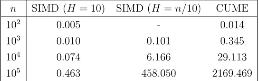
4.2. Computation time
To demonstrate the improvement in the performance of the two algorithms we run model I, withp= 10 andn = 102,103,104,105. In one set of experiments
H = 10 and in the second set H =n/10. The results are summarized in Table 2. The computational time of SIMD is clearly shorter even in the case that
Table 2: Time in seconds to execute one iteration of SIMDLVRand CUME for different sample
sizes
n SIMD (H = 10) SIMD (H =n/10) CUME
102 0.005 - 0.014
103 0.010 0.101 0.345
104 0.074 6.166 29.113
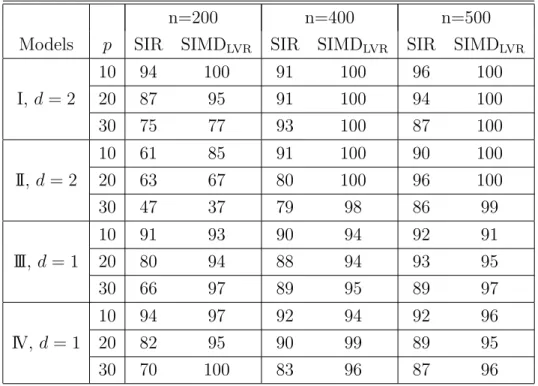
Table 3: Percentage of accurate prediction of the effective dimension by SIR and SIMDLVR.
For SIR the unifying approach developed by Bura and Yang (2011) was used. The number of slices is 10.
n=200 n=400 n=500
Models p SIR SIMDLVR SIR SIMDLVR SIR SIMDLVR
10 94 100 91 100 96 100 I, d= 2 20 87 95 91 100 94 100 30 75 77 93 100 87 100 10 61 85 91 100 90 100 II, d= 2 20 63 67 80 100 96 100 30 47 37 79 98 86 99 10 91 93 90 94 92 91 III,d = 1 20 80 94 88 94 93 95 30 66 97 89 95 89 97 10 94 97 92 94 92 96 IV, d= 1 20 82 95 90 99 89 95 30 70 100 83 96 87 96
we use a huge number of slices. Although not shown we emphasize that the performance of SIMD is not affected by the different number of slices and it is very close to CUME for all sample sizes n (even whenH = 10).
4.3. Performance for order determination
We run a simulation to compare the performance of the sequential tests de-veloped in the previous section for the SIMDLV R. We compare the performance
of those tests with the tests developed for SIR in Bura and Cook (2001). We use models I, II . We also include Model III:Y = X1+X2+σε,Model IV:Y =
X1/[0.5 + (X1+ 1)2] +σε. The effective dimension for models III and IV isd= 1
and for models I and II the effective dimension is d = 2. The results are sum-marized in Table 3 where only the results for test statistic Tsc are presented for
4.4. Categorical responses
Table 4: First direction coefficients for SIMDOVA and CUME for the Iris data under order 1
(setosa=1, versicolor=2, viginica=3) and order 2 ((setosa=2, versicolor=1, viginica=3)). The last row gives the distance between the two SIMDOVA vectors and the distance between the
two CUME vectors
SIMDOVA CUME
Variables Order 1 Order 2 Order 1 Order 2 Petal Length -0.150 -0.150 -0.149 -0.091
Petal Width -0.148 -0.148 -0.066 0.188
Sepal Length 0.851 0.851 0.714 0.063
Sepal Width 0.481 0.481 0.681 0.976
Distance dist=1 dist=0.505
We use the Iris data to demonstrate the advantage of SIMDOVAwith
categor-ical responses. The dataset consists of 150 observations, 50 from each of setosa, versicolor, virginica species of iris flower. For each flower petal length and width and sepal length and width are measured. Since there is no natural ordering of the species we run the OVA algorithm and CUME using two different orderings of the species. In the first run setosa, versicolor and virginica are coded as 1, 2, 3 respectively and in the second they are coded as 2, 1, 3 respectively. Table 4 shows the first direction extracted by each method for each ordering. It is clear that for OVA there is no difference, while there is a big difference for CUME. The distance measured is based on the trace correlation in (10).
5. Discussion
In this work we use the differences of inverse means to achieve sufficient dimension reduction. We present two different algorithms to achieve this. The first algorithm, called LVR, is theoretically equivalent to CUME by Zhu, Zhu and Feng (2010) but has certain advantages. First, when the number of obser-vations is really large it is estimating the CS faster than CUME as it uses much less cutoff points. Also if it is compared to SIR it is more robust to the number of slices. The second algorithm, called OVA, is shown to solve the issue CUME has when the response is categorical with no logical ordering between its values.
We believe similar algorithms can be developed for SAVE and DR algo-rithms. Since those two methods use conditional second moments we believe they require different methods treatment as one should make sure some proper-ties of covariance matrices are not affected by using functions of two covariance matrices.
Acknowledgements
We are very grateful to an associate editor, a referee and Dr. Jonathan Gillard, whose many useful comments and suggestions greatly broadened the results of this manuscript.
References
1. Bache, K. and Lichman, M. (2013). UCI Machine Learning Reposi-tory [http://archive.ics.uci.edu/ml]. Irvine, CA: University of California, School of Information and Computer Science.
2. Bentler, P. M. and Xie, J. (2000). Corrections to test statistics in principal Hessian directions. Statistics and Probability letters, 47, 381–389.
3. Bura, E. and Cook, D. R. (2001). Extending SIR: the weighted chi-square test. Journal of the American Statistical Association, 96, 996–1003. 4. Bura, E. and Pfeiffer, R. (2008). On the distribution of the left singular
vectors of a random matrix and its applications. Statistics and Probability Letters,78, 2275–2280.
5. Bura, E. and Yang, J. (2011). Dimension estimation in sufficient dimen-sion reduction: A unifying approach. Journal of Multivariate Analysis,
102, 130–142
6. Cook, R. D. (1998a). Regression Graphics: Ideas for Studying Regressions through Graphics. New York: Wiley.
7. Cook R. D. (1998b). Principal Hessian directions revisited (with discus-sion). Journal of the American Statistical Association,93, 84 – 100. 8. Cook, R. D. and Li, B. (2002). Dimension reduction for the conditional
mean in regression. The Annals of Statistics, 30, 455–474.
9. Cook, R. D. and Weisberg, S. (1991). Discussion of “Sliced inverse re-gression for dimension reduction”. Journal of the American Statistical Association, 86, 316–342.
10. Ferr´e, L. (1998). Determining the Dimension in Sliced Inverse Regression and related methods. Journal of the American Statistical Association,93, 132–140.
11. Horton, P. and Nakai, K. (1996). A Probablistic Classification System for Predicting the Cellular Localization Sites of Proteins. Intelligent Systems in Molecular Biology,4, 109–115.
12. Li, B., Artemiou, A. and Li L. (2011). Principal Support Vector Machine for linear and nonlinear sufficient dimension reduction. The Annals of Statistics, 39, 3182–3210
13. Li, B. and Wang, S. (2007). On directional regression for dimension re-duction. Journal of the American Statistical Association, 102, 997–1008. 14. Li, B., Zha, H., and Chiaromonte, F. (2005). Contour regression: a general approach to dimension reduction. The Annals of Statistics,33, 1580-1616. 15. Li, K. -C. (1991). Sliced inverse regression for dimension reduction (with discussion). Journal of the American Statistical Association, 86, 316 – 342.
16. Li, K. -C. (1992). On principal Hessian directions for data visualization and dimension reduction: another application of Stein’s lemma. Journal of the American Statistical Association, 86, 316 – 342.
17. Saracco, J. (1997). An asymptotic theory for sliced inverse regression.
Communication in Statistics - Theory and Methods, 29, 2141–2171 18. Schott, J. R. (1994). Determining the dimensionality in sliced inverse
regression. Journal of the American Statistical Association,89, 141–148. 19. Shao, Y. Cook, R. D. and Weisberg, S. (2007). Marginal tests with sliced
average variance estimation. Biometrika,94, 285–296.
20. Velilla, S. (1998). Assessing the number of linear components in a general regression problem. Journal of the American Statistical Association, 93, 1088–1098.
21. Yin, X., Li, B. and Cook, R. D. (2008). Successive direction extraction for estimating the central subspace in a Multiple-index regression. Journal of Multivariate Analysis, 99, 1733–1757.
22. Zhu L. P., Zhu L. X. and Feng Z. H. (2010) Dimension Reduction in Re-gression through Cumulative Slicing Estimation Journal of the American Statistical Association, 105, 1455-1466.