Genetic Programming
by
Kourosh Neshatian
A thesis
submitted to the Victoria University of Wellington in fulfilment of the
requirements for the degree of Doctor of Philosophy in Computer Science. Victoria University of Wellington
Feature manipulation refers to the process by which the input space of a machine learning task is altered in order to improve the learning quality and performance. Three major aspects of feature manipulation are feature construction, feature ranking and feature selection. This thesis proposes a new filter-based methodology for feature manipulation in classification problems using genetic programming (GP). The goal is to modify the input representation of classification problems in order to improve classification performance and reduce the complexity of classification models.
The thesis regards classification problems as a collection ofvariables in-cludingconditionalvariables (input features) anddecisionvariables (target class labels). GP is used to discover the relationships between these vari-ables. The types of relationship and the ways in which they are discovered vary with the three aspects of feature manipulation.
In feature construction, the thesis proposes a GP-based method to con-struct high-level features in the form of functions of original input fea-tures. The functions are evolved by GP using an entropy-based fitness function that maximises the purity of class intervals. Unlike existing algo-rithms, the proposed GP-based method constructs multiple features and it can effectively perform transformational dimensionality reduction, using only a small number of GP-constructed features while preserving good classification performance.
In feature ranking, the thesis proposes two GP-based methods for rank-ing srank-ingle features and subsets of features. In srank-ingle-feature rankrank-ing, the proposed method measures the influence of individual features on the classification performance by using GP to evolve a collection of weak clas-sification models, and then measures the contribution of input features to
structure for GP trees and a new binary relevance function is proposed to measure the relationship between a subset of features and the target class labels. It is observed that the proposed method can discover complex relationships—such as multi-modal class distributions and multivariate correlations—that cannot be detected by traditional methods.
In feature selection, the thesis provides a novel multi-objective GP-based approach to measuring the goodness of subsets of features. The subsets are evaluated based on their cardinality and their relationship to target class labels. The selection is performed by choosing a subset of fea-tures from a GP-discovered Pareto front containing suboptimal solutions (subsets). The thesis also proposes a novel method for measuring the re-dundancy between input features. It is used to select a subset of relevant features that do not exhibit redundancy with respect to each other.
It is found that in all three aspects of feature manipulation, the pro-posed GP-based methodology is effective in discovering relationships be-tween the features of a classification task. In the case of feature construc-tion, the proposed GP-based methods evolve functions of conditional vari-ables that can significantly improve the classification performance and re-duce the complexity of the learned classifiers. In the case of feature rank-ing, the proposed GP-based methods can find complex relationships be-tween conditional variables and decision variables. The resulted rank-ing shows a strong linear correlation with the actual classification perfor-mance. In the case of feature selection, the proposed GP-based method can find a set of sub-optimal subsets of features which provids a trade-off between the number of features and their relevance to the classification task. The proposed redundancy removal method can remove redundant features from a set of features. Both proposed feature selection methods can find an optimal subset of features that yields significantly better clas-sification performance with a much smaller number of features than con-ventional classification methods.
Produced Publications
1. Kourosh Neshatian, Mengjie Zhang, and Mark Johnston. “Feature Construction and Dimension Reduction Using Genetic Programming”. Proceedings of the 20th Australian Joint Conference on Artificial Intelli-gence (AI’07), Lecture Notes in Artificial IntelliIntelli-gence, Vol. 4830, Springer, Gold Coast, Australia, December 2007. pp 160-170.
2. Kourosh Neshatian and Mengjie Zhang. “Genetic Programming and Class-Wise Orthogonal Transformation for Dimension Reduction in Classification Problems”. Proceedings of the 11th European Conference on Genetic Programming (EuroGP 2008), Lecture Notes in Computer Sci-ence, Vol. 4971, Springer, Napoli, Italy, March 2008. pp 242-253. 3. Kourosh Neshatian and Mengjie Zhang. “Genetic Programming for
Performance Improvement and Dimensionality Reduction of Clas-sification Problems”. Proceedings of the 2008 IEEE World Congress on Computational Intelligence (CEC’08), IEEE Press, Hong Kong, June 2008. pp 2811-2818.
4. Kourosh Neshatian, Mengjie Zhang, and Peter Andreae. “Genetic Programming for Feature Ranking in Classification Problems”. Pro-ceedings of the seventh International Conference on Simulated Evolution and Learning (SEAL’08), Lecture Notes in Computer Science, Vol. 5361, Springer, Melbourne, Australia, December 2008. pp 544-554.
5. Kourosh Neshatian and Mengjie Zhang. “Genetic Programming for Feature Subset Ranking in Binary Classification Problems”. Proceed-ings of the 12th European Conference on Genetic Programming (EuroGP 2009), Lecture Notes in Computer Science, Vol. 5481, Springer, Tbingen, Germany, April 2009. pp 121-132.
6. Kourosh Neshatian and Mengjie Zhang. “Pareto Front Feature Se-lection: Using Genetic Programming to Explore the Feature Space1”.
Proceedings of the 11th Annual Conference on Genetic and Evolutionary Computation (GECCO’09), ACM Press, Montreal, Qubec, Canada, July 2009. pp 1027-1034.
7. Kourosh Neshatian and Mengjie Zhang. “Unsupervised Elimination of Redundant Features Using Genetic Programming2”.Proceedings of
the 22nd Australasian Joint Conference on Artificial Intelligence (AI’09), Lecture Notes in Artificial Intelligence, Vol. 5866, Springer, December 2009. pp 432-442.
8. Kourosh Neshatian and Mengjie Zhang. “Dimensionality Reduction in Face Detection: A Genetic Programming Approach3”. Proceedings
of the 24th International Conference on Image and Vision Computing, IEEE Press, Wellington, New Zealand, November 2009. pp 391-396. 1The paper was nominated for the best paper award.
2The paper has received the best student paper award.
3The paper investigates one of the possible future directions of the thesis. The research
Acknowledgments
I would like to express my gratitude to those who gave me the assistance and support I needed to complete this thesis.
My thanks goes to my advisers, A/Prof. Mengjie Zhang for his su-pervision, guidance and attention to detail throughout the course of my research, and Dr. Peter Andreae for his constructive and often motivating remarks and the many interesting discussions.
I must acknowledge the financial assistance of Victoria University of Wellington (Victoria PhD Scholarships and Marsden Fund VUW0806) with-out which the past three years would have been far more stressful and accompanied by far fewer Lattes and Mochaccinos.
And finally, my appreciation to all those, especially friends and fellow researchers from the School of Computer Science, who made my time at Victoria University of Wellington an experience that went beyond my ex-pectations.
Contents
1 Introduction 1
1.1 Motivations . . . 1
1.2 Goals . . . 3
1.3 Major Contributions . . . 4
1.4 Organisation of the Thesis . . . 6
1.4.1 Structure . . . 6
1.4.2 Outline . . . 6
1.4.3 Navigation . . . 8
1.5 Benchmark Problems for Evaluation . . . 8
1.6 Notation . . . 9
2 Literature Review 11 2.1 Machine Learning . . . 11
2.1.1 Classification Algorithms . . . 12
2.1.1.1 Training and Testing . . . 12
2.1.1.2 Representation . . . 13
2.1.1.3 Decision Tree Classifiers . . . 14
2.1.1.4 Support Vector Machines . . . 14
2.1.1.5 Bayesian Classifiers . . . 15
2.1.1.6 Other Classification Techniques . . . 15
2.2 Feature Manipulation . . . 16
2.2.1 Fundamental Concepts . . . 16
2.2.1.1 Basic Operations . . . 16 iv
2.2.1.2 Wrapper vs Filter Approach . . . 17
2.2.2 Feature Construction . . . 18
2.2.2.1 Classical Methods for Feature Construction 18 2.2.3 Feature Selection . . . 18
2.2.3.1 Wrappers for Feature Selection . . . 19
2.2.3.2 Filters for Feature Selection . . . 20
2.2.4 Feature Ranking . . . 20
2.2.4.1 Issues with Epistatic Features . . . 21
2.2.5 Transformational Dimensionality Reduction . . . 22
2.3 Genetic Programming . . . 23
2.3.1 Overview of Evolutionary Computation . . . 23
2.3.1.1 Evolutionary Algorithms . . . 23
2.3.1.2 Swarm Intelligence . . . 25
2.3.2 GP Algorithm . . . 25
2.3.3 Program Representation . . . 26
2.3.4 Creating Initial Populations . . . 27
2.3.5 Genetic Operators . . . 28
2.3.5.1 Crossover . . . 28
2.3.5.2 Mutation . . . 29
2.3.5.3 Reproduction . . . 30
2.3.6 Fitness Function and Selection Mechanism . . . 31
2.4 GP for Feature Manipulation . . . 31
2.4.1 A Generic Outline . . . 32
2.4.2 GP for Feature Construction . . . 33
2.4.2.1 Wrapper Approaches to Using GP for Feature Construction 34 2.4.2.2 Filter Approaches to Using GP for feature Construction 34 2.4.3 GP for Feature Selection . . . 35
2.5 Summary and Discussion . . . 35
3 Multiple Feature Construction 37 3.1 Introduction . . . 37
3.1.1 Defining Feature Construction . . . 37
3.1.2 The Appropriateness of Genetic Programming . . . . 38
3.1.3 Wrapper Approach vs Filter Approach . . . 38
3.1.4 Chapter Goals . . . 39
3.2 Developing a Measure of Goodness . . . 39
3.2.1 Decision Stump and Its Limitation . . . 40
3.2.2 Extending Decision Stumps to Class Intervals . . . . 42
3.3 Proposing a Non-Wrapper Fitness Function . . . 44
3.3.1 Class Intervals: A Mathematical Model . . . 45
3.3.1.1 Intervals of Classes with Normally Distributed Instances 45 3.3.1.2 Intervals of Classes with Unknown Distributions 45 3.3.2 Purity Measure: A Mathematical Model . . . 46
3.3.2.1 Using Shannon’s Entropy . . . 47
3.3.3 The Fitness Function . . . 48
3.3.3.1 Finding a Class Interval: The Algorithm . . 49
3.3.3.2 Fitness Evaluation: Measuring the Entropy 51 3.4 A GP System for Feature Construction . . . 53
3.4.1 System Diagram . . . 53 3.4.2 The GP Search . . . 53 3.5 Empirical Results . . . 56 3.5.1 Design of Experiments . . . 56 3.5.1.1 Datasets . . . 56 3.5.1.2 GP Settings . . . 56 3.5.1.3 Evaluation Process . . . 58
3.5.2 Results and Analysis . . . 59
3.5.2.1 Classification Performance Using Augmented Datasets 59 3.5.2.2 Classification Performance Using Only Constructed Features 62 3.5.2.3 Effect of Constructed Features on Decision Tree Complexity 63 3.5.2.4 Analysis of A GP-Constructed Feature . . . 65
4 Dimensionality Reduction 69
4.1 Introduction . . . 69
4.1.1 Transformational Reduction . . . 69
4.1.2 Challenges in Dimensionality Reduction using GP . . 70
4.1.3 Chapter Goals . . . 71
4.2 Enriching GP Material through Transformations . . . 72
4.2.1 Finding a Promising Transformation . . . 72
4.2.1.1 The Issue of Oblique Class Boundaries in Decision Trees 72 4.2.1.2 Limitations of PCA in Classification Problems 73 4.2.1.3 Class-wise Orthogonal Transformation . . . 76
4.2.2 A Real World Example . . . 79
4.2.3 The Enrichment Process . . . 82
4.2.3.1 Two Options for Using Transformations as Genetic Material 82 4.2.3.2 Extended Variable Terminal Sets . . . 84
4.2.3.3 Enrichment Algorithm . . . 85
4.3 The Fitness Function . . . 86
4.3.1 A Generalised Model: Renyi’s Entropy . . . 88
4.3.2 A Simple and Efficient Model . . . 88
4.3.3 Algorithm . . . 89
4.4 A GP System for Dimensionality Reduction . . . 91
4.4.1 Algorithm . . . 93 4.5 Empirical Results . . . 93 4.5.1 Design of Experiments . . . 93 4.5.1.1 Datasets . . . 95 4.5.1.2 GP Settings . . . 95 4.5.1.3 Evaluation Process . . . 96
4.5.2 Results and Analysis . . . 98
4.5.2.1 Effectiveness of the Algorithm . . . 98
4.5.2.2 Comparison with the PCA method . . . 101
5 Single-Feature Ranking 104
5.1 Introduction . . . 104
5.1.1 Motivations . . . 104
5.1.2 GP Suitability for Feature Ranking . . . 105
5.1.3 Chapter Goals . . . 105
5.2 GP-based Single-Feature Ranking . . . 106
5.2.1 The Main Idea . . . 106
5.2.2 Overall System Diagram . . . 107
5.3 Using GP to Build Weak Classifiers . . . 108
5.3.1 Classification Model . . . 109
5.3.2 GP Algorithm and the Fitness Function . . . 110
5.4 Ranking Features . . . 112 5.4.1 Algorithm . . . 113 5.5 Empirical Results . . . 115 5.5.1 Design of Experiments . . . 115 5.5.1.1 Datasets . . . 116 5.5.1.2 GP Settings . . . 116 5.5.1.3 Evaluation Process . . . 118 5.5.2 Results . . . 119
5.5.2.1 Scores and Ranks . . . 119
5.5.2.2 Effectiveness of GP-based Ranking: Comparison to the Baseline119 5.5.2.3 Utility in Dimensionality Reduction . . . 121
5.6 Summary and Discussion . . . 126
6 Ranking Subsets of Features 130 6.1 Introduction . . . 130
6.1.1 Chapter Goals . . . 131
6.2 GP for Ranking Subsets of Features . . . 132
6.2.1 Overview . . . 132
6.2.2 Program Trees: A Virtual Structure . . . 132
6.2.4 Fitness Function . . . 136
6.2.5 Case Studies . . . 139
6.2.5.1 Bimodal Class Distribution . . . 139
6.2.5.2 Correlated Features . . . 141
6.3 Exploring the Search Space of Subsets of Features . . . 142
6.3.1 Search Space Topology . . . 142
6.3.2 Difficulties in Exploring the Search Space . . . 143
6.3.3 Improving Search Space Exploration . . . 145
6.4 Creating a Pareto Front . . . 148
6.4.1 Feature Selection Objectives . . . 148
6.4.2 Pareto Archive . . . 149
6.5 The Main System . . . 150
6.6 Empirical Results . . . 152
6.6.1 Design of Experiments . . . 152
6.6.1.1 Datasets . . . 153
6.6.1.2 GP Settings and Implementation Details . . 153
6.6.1.3 Evaluation . . . 155
6.6.2 Results . . . 155
6.6.2.1 Subset Ranking . . . 155
6.6.2.2 The Relation between the Highest-Rank and the Best Subset of Featur 6.6.2.3 Search Space Exploration . . . 159
6.6.2.4 Subset Selection . . . 160
6.7 Summary and Discussion . . . 163
7 Elimination of Redundant Features 165 7.1 Introduction . . . 165
7.1.1 Chapter Goals . . . 166
7.2 Primary Concepts . . . 167
7.2.1 Redundant Features . . . 167
7.2.2 Degrees of Redundancy . . . 168
7.3.1 A GP-based Redundancy Measure . . . 170
7.3.2 A Synthetic Example . . . 172
7.3.3 Algorithm . . . 174
7.4 Feature Selection . . . 175
7.4.1 System Diagram . . . 175
7.4.2 Forward Selection Algorithm . . . 177
7.5 Empirical Results . . . 179
7.5.1 Design of Experiments . . . 179
7.5.1.1 Datasets . . . 179
7.5.1.2 GP Settings and Implementation Details . . 179
7.5.1.3 Evaluation . . . 181
7.6 Results and Analysis . . . 181
7.7 Summary and Discussion . . . 186
8 Conclusions 188 8.1 Achieved Objectives . . . 188
8.2 GP and Feature Manipulation . . . 189
8.2.1 GP for Feature Construction . . . 190
8.2.1.1 Improvements to the Classification Performance190 8.2.1.2 The Richness of GP-Constructed Features and Transformational Dimensionality 8.2.1.3 Reduction in the Complexity of Classification Models191 8.2.1.4 The Effect of Enrichment of Genetic Material on the Quality of Solutions 8.2.2 GP for Feature Ranking . . . 192
8.2.2.1 Dimensionality Reduction via Using a few High-Rank Features192 8.2.2.2 Deterioration in Classification Performance due to Excessive Number 8.2.2.3 Finding the Complicated Relationships between Groups of Input Featur 8.2.2.4 High Positive Linear Correlation between Provided Ranking and Actual 8.2.3 GP for Feature Selection . . . 193
8.2.3.1 Finding the Best Subset of Features through High-Rank Subsets193 8.2.3.2 Finding Optimal Subsets of Features on a Pareto Front194
8.2.3.4 Improving Classification Performance through Removing Redundant 8.3 Impact and Utilisation of Findings . . . 195
8.3.1 Improving the Performance of Symbolic Learners in Numeric Domains195 8.3.2 More Promising Transformational Dimensionality Reduction196
8.3.3 Improved Feature Selection by Subset Ranking . . . . 197
8.3.4 A New Way of Detecting and Removing Redundant Features198 8.4 Future Directions . . . 198
8.4.1 Directions in Using GP for Feature Construction . . . 198
8.4.1.1 Handling Nominal Features and Features with Missing Values198 8.4.1.2 Cooperative Co-Evolutionary Multiple Feature Construction199 8.4.1.3 Further Enrichment of Genetic Material . . 199
8.4.1.4 Testing the Proposed Algorithm on Other Classifiers199 8.4.2 Directions in Using GP for Feature Ranking . . . 200
8.4.2.1 Making GP Capable of Using Very Large Numbers of Features in Pr 8.4.3 Directions in Using GP for Feature Selection . . . 200
8.4.3.1 Testing the Proposed GP-based Methods on Other Datasets200 8.4.3.2 A Complete GP Ranking and Redundancy Removal System200 8.4.3.3 Using GP to Explore the Feature Lattice Directly201
8.4.3.4 Using the GP-Based Algorithms on Problems with Large Numbers
A Benchmark Datasets 202
List of Tables
1.1 The coverage and dependency of the content of the thesis . . 8
1.2 The classification problems used throughout the thesis . . . 9
3.1 Specification of datasets used in experiments. . . 57
3.2 GP Settings . . . 58
3.3 Evaluation Settings . . . 59
3.4 Number of features at different stages . . . 60
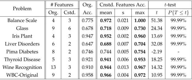
3.5 Classification accuracy over the original and augmented dataset 61 3.6 Results of the proposed approach and the basic decision tree approach. 63 3.7 Changes in Complexity of Decision Trees . . . 64
4.1 Specification of datasets used in experiments . . . 96
4.2 GP Settings . . . 97
4.3 Evaluation Settings . . . 98
4.4 Dimensionality reduction . . . 99
4.5 Classification performance before and after dimensionality reduction100 4.6 Classification Performance . . . 102
5.1 Specifications of datasets used in experiments . . . 116
5.2 GP Settings . . . 117
5.3 Evaluation Settings . . . 118
5.4 Feature ranks . . . 119
6.1 Three relevance measures on two case studies . . . 139
6.2 Specifications of datasets used in experiments . . . 153
6.3 GP Settings . . . 154
6.4 Evaluation Settings . . . 155
6.5 Correlation between GP-calculated relevance and classification performance158 6.6 Selection Gain . . . 159
6.7 Classification Results . . . 162
7.1 GP Settings . . . 180
7.2 Evaluation Settings . . . 181
7.3 Corrected ranking based on different redundancy thresholds (θ)182 7.4 Number of eliminated redundant features . . . 184 7.5 Performance of the J48 classifier using the selected features . 185 7.6 Performance of the SVM classifier using the selected features 186
List of Figures
2.1 A feature manipulation system taking a wrapper approach. 17
2.2 A Sample Tree-based Genetic Program . . . 27
2.3 Crossover Operator in Tree-based GP . . . 29
2.4 Mutation Operator in Tree-based GP . . . 30
2.5 The outline of the feature creation process using GP. . . 32
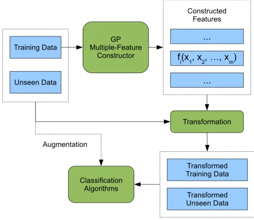
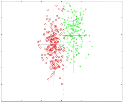
3.1 The goodness of a featurexform the viewpoint of a decision stump: (a) the feature 3.2 The goodness of a featurexfrom the viewpoint of a class interval: (a) the feature is 3.3 An example featurexand an interval for class+. The class interval creates a new pr 3.4 The system diagram of the proposed GP-based multiple-feature construction system 3.5 A learnt decision tree using a constructed feature,yB. The feature has been constructed 4.1 An artificial dataset with two original features,x1andx2, and two classes,+and◦. 4.2 The PCA transformation of the data displayed in the previous figure. 75 4.3 Transformed input space using class-wise orthogonal transformations 78 4.4 Thyroid disease dataset represented in two dimensions. The axes are two attributes 4.5 Transformed input space of the Thyroid problem using PCA. The axes are the two principle 4.6 Two (out of six) dimensions presented after transforming the original input space of 4.7 An overview of the genetic material enrichment process and dimensionality reduction. 4.8 Overview of the proposed GP-based dimensionality reduction system. 92 5.1 Overview of the system. . . 108
5.2 Score of features in the Ionosphere, Sonar and WBC-Diagnostic120
5.3 Comparison of the proposed ranking with the baseline (random selection) in the Ionospher xiv
5.4 Comparison of the proposed ranking with the baseline (random selection) in the Sonar
5.5 Comparison of the proposed ranking with the baseline (random selection) in the WBC-Diagnostic 5.6 Accuracy of different classifiers in the John Hopkins University Ionosphere classification
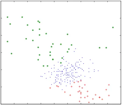
5.7 Accuracy of different classifiers in the Sonar classification task by using different numbers 5.8 Accuracy of different classifiers in the WBC-Diagnostic classification task by using dif 6.1 A virtual structure for a GP program for measuring the usefulness of a subset of featur 6.2 Magnitude of parameterβin LR (top) andBRfunction (bottom) with respect to the 6.3 A bimodal class distribution along featurexin a binary classification problem (Left). 6.4 A binary classification task presented with respect to two of its features,xandy, which 6.5 Search space of the feature subsets in the form of a lattice where each node represents 6.6 Frequency of subsets of features in the three datasets with respect to the cardinality 6.7 An artificial binary classification problem with classes A and B (visualised at 1 and 6.8 The diagram of the proposed GP-based subset ranking/selection system.151
6.9 Relevance of subsets of features vs. classification performance obtained by using the 6.10 Pareto front of the three datasets. . . 161
7.1 An artificial example wherex3 is redundant in the context ofx1andx2. The scatter 7.2 A non-linear transformation function (a GP program) that can detect the redundancy 7.3 Diagram of a feature selection system using GP to evaluate redundancy.177
List of Algorithms
1 F ind-Interval(y,c, c⋆): Finding the Interval of a Class . . . 50
2 M F C-F itness(X, φ, c⋆): Evaluating the Fitness of a Constructed Feature 52
3 GP-M ultiple-F eature-Constructor(D): Constructing Multiple Features: A Filter Appr 4 Create-Extended-Dataset(D): Genetic Material Enrichment: Creating an Extended Dataset 5 DR-F itness(D+, φ, c⋆): Evaluating Fitness in Dimensionality Reduction 90
6 GP-based-Dimensionality-Reduction(D): Transformational Dimensionality Reduction 7 Evolve-W eak-Classif ier(D, c⋆): Evolving Weak Classifiers . . 111
8 GP-based-Single-F eature-Ranking(D): Single-Feature Ranking114 9 BR-F itness(D, φ): Evaluating Fitness through Binary Correlation138 10 M easure-Redundancy(x,A, θ): Measuring Redundancy . . . . 176
11 F orward-Selection(X,r, m⋆, θ): Redundancy Elimination through Forward Selection
Chapter 1
Introduction
This thesis proposes a new methodology that uses genetic programming for feature manipulation. Feature manipulation refers to the process by which the input space of a machine learning task is altered in order to im-prove the learning quality and performance. Alterations to the input space are made by means of constructing higher-level features, selecting infor-mative features, and removing redundant or noisy features. Traditional solutions for feature manipulation such as linear transformation of the in-put space, single feature construction, individual feature ranking, and the likes are highly problem-dependent and domain-specific. They usually make assumptions that do not necessarily hold across different problems. The thesis addresses these issues by taking an evolutionary approach to searching through the space of functions and actions that can be applied to features using genetic programming.
1.1
Motivations
From an abstract point of view, machine learning solutions address two fundamental design commitments: representation and reasoning. A rep-resentation system provides a formalism to represent different aspects of the real world (problem domain) while a reasoning system deals with the
process of learning and predicting future states of the system [130]. Ob-viously, the quality of these two systems has a significant impact on the level of attainment in machine learning.
Inductive learning, where an agent learns from a set of observations, is a widely-practiced paradigm of machine learning. Increasing the qual-ity of representation in this paradigm is usually carried out through some improvements to the input space [14]. In some learners, representational improvements are dealt with intrinsically as part of the learning process— for example, neural networks can implicitly build new features based on the input signals in their hidden layers. However, for many others like de-cision trees, there is no such implicit way of improving the representation as part of the learning process. For the latter category, therefore, explicit improvements to the input space are required to increase the learning per-formance.
The goal offeature manipulationis to improve the representation system by making changes to the feature space. Feature manipulation includes: feature construction, feature ranking and feature selection [89]. Feature construction is a means of enhancing the quality of representation by cre-ating higher-level features as a function of the original features. Feature selectionis the task of finding a minimal subset of the original features that is sufficient to describe the target concepts. Feature selection is a treatment forthe curse of dimensionality. It leads to dimensionality reduction by elim-inating unnecessary and redundant features from the problem, which in turn improves the learning performance. Learnt models induced by using smaller numbers of features are also easier to interpret. Feature ranking is an avenue to feature selection that imposes a ranking over features, rep-resenting their relative importance; the user usually chooses the desired number of features to be selected from a ranking scheme.
Genetic programming(GP) is an evolutionary search paradigm [71]. GP provides a flexible and expressive tool for dynamically building programs and functions. Given a set of primitive functions (or actions) and an
objec-tive function, GP is able to build different types of programs, ranging from mathematical expressions to complete classification models. This flexibil-ity of GP in searching complicated search spaces motivates this paradigm a promising choice for non-trivial problems like feature manipulation.
There has been a growing trend in using GP for feature manipulation, particularly for feature construction, with very promising results. Unlike traditional feature construction algorithms—for example, principle com-ponent analysis—which come with certain assumptions and constraints and are limited to certain types of transformation, GP has been able to build a variety of transformations without being bound to any predefined templates. In the feature construction domain, GP has been successfully used to construct high-level features that boost the performance of clas-sifiers. GP can be used in different feature construction scenarios: along with evolving a classifier [105, 80, 10], as a pre-processing phase [120], or in embedded solutions [30].
The current state of the art in using GP for feature manipulation is somewhat limited compared to the potential of GP. Most of the research in feature construction take a wrapper approach which is learner specific and computationally very intensive. Those research works that take a fil-ter(non-wrapper) approach are limited to constructing one single feature [43, 104]. Research in feature selection and feature ranking using GP is quite young and limited to only a few works. Details of feature manipula-tion using GP are presented in Chapter 2. The aim of this thesis is to deal with the current challenges in this area.
1.2
Goals
The overarching goal of this thesis is to investigate a new approach to the use of GP for feature manipulation in classification tasks. This goal can be broken down to:
– using GP for feature construction;
– using GP for transformational dimensionality reduction;
• using GP for feature selection:
– using GP for ranking single features and groups of features; – using GP for detecting feature redundancy.
Given a classification task presented with a set of conditional features (input features) and decision features (class labels), to achieve the above-mentioned goals, the thesis has to find possible answers to the following research question:
How can genetic programming be used to discover the rela-tionships between the features of a classification task?
When the goal is feature transformation, we need to use GP to discover the relationship between conditional features and decision features by con-structing higher-level features. When the goal is feature selection, we need to use GP to discover the functional relationships between conditional fea-tures and decision feafea-tures, and the mutual relationships amongst condi-tional features.
1.3
Major Contributions
The thesis has made the following major contributions:
• The thesis proposes a GP-based multiple feature construction sys-tem. Unlike many existing filter-based GP systems that can only construct a single feature, the proposed system is capable of making multiple high-level features without wrapping any other classifica-tion algorithms for fitness evaluaclassifica-tion. The constructed features are evolved as functions of original features. A family of entropy-based
fitness functions are introduced which are used by the GP search. A new transformation technique that increases the chance of find-ing new high-level discriminatfind-ing features is proposed. Our results on several benchmark problems show that the proposed method can significantly improve the classification performance of the problems while reducing the dimensionality and the complexity of the learnt models. These results have been partly published in [114, 109, 113].
• The thesis proposes a GP-based single feature ranking system. The system uses GP to find the relationship between features and target classes and then, based on the strength of the relationship, ranks in-dividual features. The ranking provided by the system shows strong connections to the actual importance of features [108].
• The thesis proposes a GP-based system for measuring the relevance of subsets of features to target concepts in a binary classification task. A virtual program structure and an evaluation function are intro-duced in a way that constructed GP programs can measure the good-ness of subsets of features. The proposed system can detect relevant subsets of features in situations where other ranking methods have difficulties, such as multimodal class distributions and mutually cor-related features. The GP search results form a Pareto space in which feature selection is performed [110, 111].
• The thesis shows how GP can be used to find complex relationships between groups of features that cannot be found by traditional tech-niques. The method is used to measure the quotient of redundancy between features. We then introduce an algorithm that employs the GP-based redundancy detection system to perform feature selection by removing redundant features and irrelevant features [112].
1.4
Organisation of the Thesis
1.4.1
Structure
The main contributions of the thesis are presented in Chapters 3–7. Each chapter addresses some of the subgoals of the thesis by finding solutions for the central research questions of the thesis. All five chapters share the same high-level structure: each chapter starts by proposing some theoreti-cal solutions followed by corresponding algorithms and diagrams. At the end of each chapter, the proposed system is tested and evaluated against a number of benchmark problems and the empirical results are analysed and discussed.
1.4.2
Outline
Chapter 2 carries out a review of the literature on feature manipulation, focusing on evolutionary approaches. The review covers the fundamental concepts of feature manipulation including feature construction, ranking and selection. It also visits the basics of evolutionary algorithms and ge-netic programming. It covers recent advances in feature manipulation us-ing GP and discusses open questions and current challenges that form the motivations of the thesis.
Chapter 3 proposes a GP framework for constructing multiple high-level features. It investigates the notion of discriminative features and provides an entropy-based fitness function to measure this quality. It uses the proposed system to construct multiple features for some benchmark classification tasks and evaluates the system performance.
Chapter 4 proposes some advanced topics on feature construction that are used in transformational dimensionality reduction. It investigates how the construction process can be improved by enriching the variable termi-nal set of the GP search. Class-wise orthogotermi-nal transformation is intro-duced for making encapsulating features. A simplified fitness function is
proposed that makes the GP search over large input spaces computation-ally affordable. The empirical results are presented and discussed.
Chapter 5 proposes a GP-based method for single feature ranking. It introduces a scoring mechanism which is based on the frequency of the appearance of features in high-fitness GP programs. The scoring mecha-nism is then used to rank the individual (original) features. A number of classification tasks, and a variety of classifiers restricted to just high-rank features are tested and the performance is evaluated.
Chapter 6 proposes a new method for ranking and selection of subsets of features in binary classification problems. A virtual program structure and an evaluation function are defined in a way that constructed GP pro-grams can measure the goodness of subsets of features. The outcomes of the GP search are presented in a Pareto space in which an optimum solu-tion has a maximum relevance and a minimum cardinality. The chapter then investigate how the proposed ranking for each given subset of fea-tures is correlated to the actual classification performance using that sub-set. The performance of the system is then measured via measuring the classification performance using selected subsets of features.
Chapter 7 proposes an evolutionary way of feature selection by remov-ing the redundant features from the result of a rankremov-ing algorithm. The chapter introduce a nonlinear redundancy measure which uses GP to find the redundancy quotient of a feature with respect to a subset of features. Then a forward selection algorithm is proposed which uses the proposed GP system as a redundancy measure. The effectiveness of the method is assessed by applying it to a dataset with a very large number of features.
Chapter 8 concludes the thesis by giving chapter-wise (goal-specific) conclusions and drawing overall conclusions regarding the research ques-tion. It also suggests some possible future research directions.
1.4.3
Navigation
To provide better navigation, Table 1.1 presents some information on the appearance of each of the aspects of feature manipulation and its depen-dency on chapters with the relevant background.
Table 1.1:The coverage and dependency of the content of the thesis
Chapter Aspect of Feature Manipulation Depends on
3 Construction Chapter 2
4 Construction and Reduction Chapters 2 and 3
5 Ranking Chapters 2 and 3
6 Ranking and Selection Chapters 2 and 5 (partly)
7 Selection Chapters 2 and 5 (partly)
1.5
Benchmark Problems for Evaluation
Classification problems are the main applications to which the proposed methodology in the thesis can be applied. Therefore, evaluating the method-ology involves testing it on a range of classifiers and benchmark classifica-tion problems. The choice of classifier and classificaclassifica-tion problem depends on the objective of the proposed algorithm. For example, in feature con-struction scenarios, the proposed algorithm is tested on a classifier that is not able to transform the input space by itself; in feature selection scenar-ios, where one needs to find a few good features from a large set of avail-able features, the proposed algorithms is tested on classification problems that have a relatively large number of features.
Table 1.2 shows the classifiers and classification problems that have been used in the thesis. All the datasets are available from the UCI ma-chine learning repository [6]. Appendix A provides detailed descriptions of the individual classification problems.
Table 1.2: The classification problems used throughout the thesis
Chapter Classifier(s) Benchmark Classification Problem(s) 3 Decision Tree (C4.5/J48) Balance Scale,
Glass Identification, Iris Plant, Liver Disorders, Pima Diabetes, Thyroid Disease, Wine Recognition, WBC-Original 4 Decision Tree (C4.5/J48) JH Ionosphere,
Sonar, Waveform, WBC-Diagnostic
5 Bayesian Net, JH Ionosphere,
Decision Tree (C4.5/J48), Sonar,
Naˆıve Bayes, WBC-Diagnostic
SVM (SMO)
6 Decision Tree (C4.5/J48), JH Ionosphere,
SVM (SMO) Sonar,
WBC-Diagnostic 7 Decision Tree (C4.5/J48), Isolet5
SVM (SMO)
1.6
Notation
Throughout the thesis, we follow a certain mathematical notation. We use capital letters like X for random variables or when we are talking about features in abstract. Uppercase, boldfaced letters likeX are used for ma-trices. Lowercase, boldfaced letters likexare used for vectors andx[i]
rep-resents thei-th element (or observation) of the vector. Calligraphic capital letters likeAare used for sets. The unary operator|.|is used to indicate the cardinality of a set. The list of special symbols used in the thesis follows:
m The total number of original features in a classification problem.
m⋆ The desired number of features to be selected.
F The set of all original features in a classification problem;|F|=m.
n The number of instances in the dataset.
L A scalar value showing the total number of classes (distinct class labels) in a classification problem1.
C The set of all class labels in a classification task; C =
{c1, c2, . . . , cL}and therefore|C|=L.
D A dataset containing instances. Each instance has its values for the input features and the target class labels.
φ A GP program that acts like a function; for exampley=φ(x).
I An interval of a class, whereI = (lower, upper)shows the lower and upper boundaries of the interval.
1This is the only exception to the convention of using lowercase letters for scalar
val-ues. The reason is thatIhas been frequently used in the equations and figures; a lower-caseLcould have been confusing, particularly in the figures.
Chapter 2
Literature Review
This chapter provides a review on the literature that forms the background and supports the motivations of the thesis. The chapter gives a brief in-troduction to Machine Learning and classification algorithms, the need for Feature Manipulation, and then an overview of Evolutionary Algorithms and Genetic Programming. The chapter, then, provides a detailed review of the literature on using Genetic Programming for feature manipulation. The review covers the potential and limitations of current methods for Feature Manipulation using Genetic Programming, which leads to the re-search direction adopted by the thesis.
2.1
Machine Learning
Machine learningis a major research area inartificial intelligencethat is con-cerned with designing computer programs that are capable of learning in their environment [5, 14]. Machine learning systems are expected to be able to improve their performance as they gain more experience [100]. They should change their behaviour in a way that makes them act better in future [152]. Michalski et al. [94] state that:
“Learning denotes changes in the system that are adaptive in 11
the sense that they enable the system to do the same task or tasks drawn from the same population more efficiently and more effectively the next time.”
Machine learning algorithms use a feedback mechanism to change their behaviour (learn). Depending on the type of feedback, three cases can be distinguished: supervised,unsupervised, reinforcementlearning [130]. In su-pervised learning, a set of examples in the form of different inputs and de-sired outputs are given and the goal is to learn a function that can do this input-output mapping. Inunsupervised learning, only inputs are available; the learner has to find useful patterns in the input data. In reinforcement learning, the desired outputs are not directly provided; the learner instead has to learn based on rewards and punishments it receives for its actions (outputs).
2.1.1
Classification Algorithms
Inductive learning is perhaps the most common paradigm of learning. In inductive learning, learners generalise (from observations) patterns that can distinguish positive and negative examples. Classification algorithms are a major category of inductive learning algorithms. A classifiertakes, as input, the description of an object and gives, as output, a label for the object. The set of class labels is defined as part of the problem (by users). A classifier inducer, is a supervised learning algorithm that uses a set of observations to learn ahypothesis(classifier) that can map inputs to correct class labels.
2.1.1.1 Training and Testing
The process by which a classifier inducer uses observations to learn a new classifier is called training[100]. During the training phase, the classifier inducer, is presented with observations from the problem domain called instances. The collection of instances used in the training phase is called the
training set. The algorithm learns important patterns in data by building models and adjusting the corresponding parameters. The performance of the algorithm is then tested on a collection of unseen instances, called the test set.
The learning capability of classifiers is usually evaluated by applying them to a set of benchmark problems. Benchmark problems are usually chosen from collections that are publicly accessible to researchers (e.g. UCI Machine Learning Repository [6]). Many benchmark problems do not have a specific test set. To evaluate the performance of a classifier on these problems, one should usek-fold cross-validation[100]. Ink-fold cross-validation, the dataset is randomly partitioned intok folds (partitions). In a loop of k iterations, each time one of these folds is taken as the test set and the others are used together as a training set. Thek results from the folds can then be averaged to produce a single estimate of classification performance. The advantage of this method over repeated random sub-sampling is that all observations are used for both training and validation, and each observation is used for validation exactly once. Instratifiedk-fold cross-validation, the folds are selected so that the proportion of instances from different classes, remains the same in all folds.
2.1.1.2 Representation
Instances in the training and test sets are presented to algorithms using a representation system. In the majority of learning algorithms including classification algorithms, the quality of the representation is of key impor-tance. The most common representation system is feature-value. In this system, each instance is represented in the form of a vector of values for the features defined in the problem domain. The datasets (including train-ing and test set) are usually represented in the form of a table where each row is an instance and each column represents a different feature in the problem domain. The quality of the features defined in the problem do-main, including their number and their relevance to the desired task, has
a significant effect on learning performance. 2.1.1.3 Decision Tree Classifiers
Decision treelearning is a method for approximating discrete-valued func-tions [100]. Decision trees classify instances by sorting them down the tree from the root to some label nodes. The tree is a hierarchy of nodes. For a given instance, the process starts at the root node; the value of the feature at the root node is tested and the process moves to one of the child nodes. Then the process is repeated for the subtree rooted at the new node.
There are different algorithms for learning a decision tree but the prin-ciples are the same [100]. The main question in learning a decision tree is which feature should be tested at each node of the tree. Most algo-rithms employ a top-down greedy search through the space of possible decision trees. Examples are the ID3 algorithm [126], theC4.5 algorithm [127], and its Java version, the J48algorithm [152]. These algorithms use an entropy function to measure the homogeneity of examples and choose the best node at each stage. The most important advantage of decision tree classifiers is their interpretability; learned decision trees can be trans-lated to a set of ’if-then’ rules to improve human readability. The most serious disadvantage of decision trees is perhaps their weakness in sepa-rating non-rectangular areas in the input space [127].
2.1.1.4 Support Vector Machines
Support vector machines (SVMs) form a category of statistical supervised learning algorithms. SVMs construct a number of hyperplanes in a high-or infinite-dimensional space, which are used fhigh-or classification. Instances are categorised based on what side of these hyperplanes they fall on. SVMs maximise the distances between the hyperplanes and both the nearest pos-itive and negative data points. The points that cause the boundary (hy-perplane) to fix in a particular place are referred to assupport vectors, and
a learning machine that uses such a boundary is therefore referred to as a support vector machine. The space between the boundary and the support vectors is called themargin[148].
2.1.1.5 Bayesian Classifiers
Bayesian classifiers provide a probabilistic approach to classification. Their assumption is that the behaviour of data (input-output relationships) can be captured in probability distributions [100]. Among these classifiers, Na¨ıve Bayesclassifiers are the most common and straightforward classifiers to learn. It has been shown that Na¨ıve Bayes classifiers are quite competi-tive with other classifiers such as decision trees and neural networks [95]. Na¨ıve Bayes classifiers make significant use of the assumption that all in-put features are conditionally independent. This assumption cannot be applied to many real world problems where there are some interdepen-dency between input features. Bayesian networks have been proposed as a remedy to this problems [48, 54]. Bayesian networks allow conditional independence assumptions that only apply to a subset of features.
2.1.1.6 Other Classification Techniques
In addition to the above-mentioned classification algorithms—which are used in the experiments throughout the thesis—there are many other clas-sification algorithms that are commonly used in data mining [100]. Two other important categories of classifiers are Artificial Neural Networks (ANNs) [13] and Case-based Reasoning (CBR) systems [1]. In ANNs, the information (usually in the form of numeric values) is transformed as it travels through the layers of the network. In classification problems, the network acts as a function which maps observations input space to target class labels. CBR systems are categorized aslazylearners because they do not induce any generalisation of training data until a query is received.
2.2
Feature Manipulation
Feature manipulation is an umbrella term that refers to the collection of methodologies and techniques that are practised to improve the input space of problems represented in feature-value systems [89]. This section reviews the most widely-known aspects of feature manipulation, namely feature construction,feature ranking, andfeature selection.
2.2.1
Fundamental Concepts
This subsection first explains some basic concepts that are shared among all aspects of feature manipulation.
Definition Afeatureis a function that maps entities to one of their proper-ties.
In this definition, entities are objects (observations) of the same type1and a feature represents a certain measurable property of the objects. Examples for objects of the same type are ’Ann’, ’Ben’, and ’Colin’, all being from the ’Student’ type. Examples for features are ’Height’ and ’Gender’ which correspondingly map these objects to numeric (the height of the person) and nominal (the gender of the person) values.
2.2.1.1 Basic Operations
All aspects of feature manipulation use one of the two following basic operations to make changes in the feature space of a problem.
Transformation. This process transforms the values of one or more fea-tures to a new set of values. The transformation functions are usually well-defined and deterministic. Examples of this operation are feature construction and transformational dimensionality reduction.
1In the context of learning by example and feature manipulation, the termsobservation,
Figure 2.1:A feature manipulation system taking a wrapper approach.
Selection. This process selects a subset of available features in a problem. The selected features are usually used for both the training and the testing of classification algorithms.
2.2.1.2 Wrapper vs Filter Approach
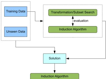
In all feature manipulation problems, when a candidate solution is found, it should be evaluated to determine its goodness and find new search di-rections. For example, one has to know how much relevant information a set of constructed/selected features can provide. There are two major approaches to evaluating a solution: wrapper and filter(or non-wrapper) [66].
Figure 2.1 shows the diagram of a feature manipulation system taking a wrapper approach. In the wrapper approach, the performance of an induction algorithm (e.g. a classifier) is used to guide the search. The wrapper approach is computationally intensive; every evaluation involves training and testing an induction algorithm.
The filter approach on the other hand, does not use any learner’s feed-back to evaluate a solution. It instead uses other heuristics that are compu-tationally more efficient. The diagram of the filter approach is very similar to that of the wrapper approach depicted in Figure 2.1. However, no in-duction algorithm is used to evaluate the solution.
2.2.2
Feature Construction
Many classification algorithms, particularly those based on symbolic learn-ing (e.g. decision rules anddecision trees), cannot achieve adequate predic-tive performance when faced with difficult real-world problems [77]. A known reason for this deficiency is the inability of these systems to make any transformations to their input spaces [100]. The issue can be partially alleviated by using feature construction as preprocessing.
2.2.2.1 Classical Methods for Feature Construction
Zheng [158] provides a review of constructive induction methods. In con-structive induction, the original features are transformed into a new space in a way that the learning performance is improved [159]. Inductive logic programming is used to construct features that can model the behaviour of data. The newly constructed features can then be used by learning al-gorithms. The constructed features can also provide some structural in-formation [142]. Hu [51] proposes a multi-strategy constructive inductive algorithm which is independent of learning algorithms.
2.2.3
Feature Selection
There are different definitions for feature selection in the literature [20]:
• Idealised: feature selection is defined to be the process of finding the minimally sized feature subset that is necessary and sufficient to model the target concept [63].
• Classical: feature selection is the process of selecting m⋆ features
from m original features, such that m⋆ < mand the value of a cri-terion function is optimised over all subsets of sizem⋆ [107].
• Improving predictive accuracy: feature selection is the process of finding a subset of features, using which either predictive perfor-mance is improved or the complexity of the model is reduced while the performance is maintained at an acceptable level [67].
• Approximating original class distribution: feature selection is the process of finding a subset of features such that the resulting class distribution, given only the selected features, approximates the orig-inal class distribution as closely as possible [67].
Overall, feature selection is the process of finding a minimal subset of features that is sufficient to solve a classification problem. Feature se-lection leads to dimensionality reduction by eliminating noisy and un-necessary features from the problem, which in turn improves the perfor-mance and makes the learning and execution processes faster. Models constructed using a smaller number of features are also easier to interpret. 2.2.3.1 Wrappers for Feature Selection
The search space of a feature selection problem has2m points wherem is
the number of original features in the problem. The search space grows exponentially with respect tom. Some wrapper approaches to feature se-lection use an external algorithm to explore this search space. The type of search algorithm could be anything from simple Hill-climbing to an evo-lutionary search [66]. The search can be towards growing an initial subset (e.g. forward selection) or towards shrinking an initial solution (e.g. back-ward elimination) [96].
Searching the collection of all 2m possible combinations of features is
search the whole space exhaustively, asmgrows, it needs to examine more points in order to find a near-optimal solution. In wrapper methods, eval-uation of candidate solutions is costly—each evaleval-uation needs a classifier to be trained and tested. Therefore, using wrapper methods on problems with a large number of original features is not always viable.
2.2.3.2 Filters for Feature Selection
Feature selection methods taking the filter approach use only data to find an optimal subset of features; they do not wrap any inductive learning algorithm (e.g. a classifier) to evaluate their solutions. FOCUSis a classi-cal filter-based feature selection algorithm that was originally defined for noise-free Boolean domains [3, 4]. It exhaustively examines all subsets of features, selects the minimal subset of features that is sufficient to deter-mine the label value for all instances in the training set.
TheReliefalgorithm is another filter method that assigns a “relevance” weight to each feature [64]. The algorithm attempts to find all relevant features. The Relief algorithm, however, does not help with redundant features [68]. Cardie [16] proposes a filter-based feature selection algo-rithm that uses a decision tree algoalgo-rithm to select a subset of features for a nearest neighbourhood algorithm. Yu [155] proposes a feature selection algorithm that takes both relevance and redundancy into account. The al-gorithm, however, is limited to problems that only have discrete features.
2.2.4
Feature Ranking
Feature ranking is an avenue to feature selection [60]. In feature ranking, a score is assigned to each solution [45]. In single (univariate) feature rank-ing, a score is associated to each feature individually and independently from other features [129]. In single feature ranking, the user selects a num-ber of high-rank features. Normally, the numnum-ber is specified by the user [46]. There are also some analytical methods to determine the best number
of features [143].
Most feature ranking methods fall into the filter approach category, and can only measure the goodness of a single feature [129, 12, 88]. This in-cludes all feature ranking measures from the information theoretic domain such as information gain (IG), gain ratio, mutual information and the likes [86].
2.2.4.1 Issues with Epistatic Features
Epistasis, a term originally from biology, is defined as interaction between genes [8]. It is used to describe how one gene can change (suppress or ex-press) the phenotypical effect of another gene. Epistasis later entered Ge-netic Algorithms (GAs) and other computational evolutionary paradigms to indicate how changing a component of a candidate solution—for ex-ample changing a bit in a GA chromosome or changing a subtree in a GP program—can change the behaviour of other components in the solution [38, 150].
Epistasis happens frequently between the features of a classification task; that is, the contribution of a feature in predicting the class label will depend on the value of some other features. Many filter methods have difficulties in handlingepistaticfeatures. The difficulties are twofold:
• The majority of filter methods cannot provide any explicit way of measuring the goodness of a group (subset) of features. These meth-ods are usually combined with a search technique to select a set of top-ranked features. However, since the features are examined indi-vidually, the selected subsets often suffer from the absence of groups of related features and the presence of redundant features.
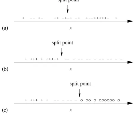
• The majority of filter methods are limited to detecting only simple types of relationships between a feature and the target class. For example, in the logistic regression model [18], the relationship is as-sumed to be linear; in most of the information theoretic measures,
it is assumed that instances can be classified by setting a split point along the feature axis.
2.2.5
Transformational Dimensionality Reduction
Although, in a sense, all feature selection algorithms perform dimension-ality reduction, the term dimensiondimension-ality reduction is most often used to refer totransformational dimensionality reduction. In transformation dimen-sionality reduction, the original features are transformed into a new space (new features). Then a small number of these transformed features is used instead of the original features [147, 9, 128]. A successful reduction in dimensionality can help in building simpler classification models. The transformations can also be useful for interpretation.
Principle component analysis (PCA) is one of the dimensionality re-duction techniques that is widely used in different applications. The goal of PCA is to linearly transform data into a more meaningful construct [37]. It can eliminate the redundancy between measurements (features), and reduce the noise by selecting more important components. This is done by diagonalizing the covariance matrix. However, as PCA is blind to the class labels in the training set, in many cases, it is not effective for classi-fication problems. Another potential drawback of PCA is that, it makes the assumption that more diversity along the axis of a generated compo-nent (feature) is a sign of being more informative and therefore it ranks generated components based on this factor. However, this assumption is certainly not always true.
From a different perspective, the problem of dimensionality reduction can be seen as a feature construction problem in which the constructed features are functions of the original features and the total number of con-structed features is sufficiently smaller than the number of original fea-tures in the problem. For example, the PCA method can be treated as a feature construction scenario in which all the constructed features are
lin-ear expressions and the objective is to find the coefficients of these poly-nomials so that PCA goals are satisfied. From this perspective, a limiting issue of PCA and many other classical dimensionality reduction methods is that they all have fixed models (e.g. linear, polynomial). These methods can only find the optimal value for theparameters(e.g. the coefficients in a polynomial model); they cannot find the right model for data by them-selves [91, 17].
2.3
Genetic Programming
This section first gives an overview of evolutionary computation and hier-archy of algorithms in this field, and then provides a more detailed review of fundamental concepts in genetic programming.
2.3.1
Overview of Evolutionary Computation
Evolutionary Computation(EC) is an area of artificial intelligence that covers the majority of nature-inspired algorithms in this field. Two main classes of these algorithms are evolutionary algorithms and swarm intelligence. 2.3.1.1 Evolutionary Algorithms
Evolutionary Algorithms (EAs) refers to a subset of algorithms in evolu-tionary computation that are generic population-based metaheuristic op-timisation algorithms. EAs use mechanisms inspired by biological evolu-tion: reproduction, mutation, recombination, and selection. Each individ-ual (member of the population) is a candidate solution. The goodness of individuals is determined by a fitness function. Evolutionary algorithms have been highly successful in solving complex problems in science and engineering [23]. Some important algorithms in this category follow.
Genetic Algorithms. Genetic Algorithms (GAs) are evolutionary search and optimisation techniques [39, 38, 49]. GAs evolve a population of chro-mosomes that can encode solutions in continuous and discrete domains. Compared to some analytical optimisation methods like gradient-based optimisation, they are less likely to be trapped in local optima. They, how-ever, tend to be computationally expensive.
Evolutionary Programming. InEvolutionary Programming (EP) a popu-lation of chromosomes is used to evolve finite-state machines (FSMs) [34]. Each FSM is in fact a program. A sequence of symbols that have been observed up to the current time is fed to each FSM. The fitness of an indi-vidual is evaluated by its ability in predicting future symbols. Like other EAs, EP uses fitness values to select individuals and then applies some evolutionary operators to find other solutions. EP has been perhaps one of the first attempts to evolve computer programs. The structure of pro-grams in EP is usually assumed to be fixed.
Evolutionary Strategies. InEvolutionary Strategies(ESs), each individual represents a fixed-length real-valued vector. The real values in the vector are parameters to a system/model that determine its behaviour. As with the bit-strings of GAs, each position in the vector corresponds to a feature of the individual. However, the features are considered to be behavioral rather than structural. Since all elements are real-valued, genetic operators can perform operations like averaging [141]. The selection of survivals in ESs is deterministic; that is, once the genetic operators are applied, a num-ber of individuals with highest fitness are selected for the next generation. Genetic Programming. Genetic programming (GP) is a sophisticated EA which is used to evolve a computer program that performs a desired task [71, 74, 73, 75]. GP has been highly successful as a technique for getting computers to automatically solve problems without having to tell them
explicitly how. It has proved to be applicable and effective in a variety of fields from planning and discovery of game-playing strategies to symbolic regressions and evolving classification systems.
2.3.1.2 Swarm Intelligence
Swarm Intelligence(SI) algorithms are inspired by the collective intelligence of social insects. SI systems are typically composed of simple interacting individuals and the intelligence lies in the networks of interactions among individuals, and between individuals and the environment [15]. Two main algorithms in SI areant colony optimisation(ACO) andparticle swarm opti-misation(PSO). ACO is a class of optimisation algorithms modeled based on the behaviour of ant colonies [24]. ACO methods are useful in prob-lems that need to find paths to goals. PSO is a simple search method in which solutions are represented by inter-communicating particles [62]. Particles are influenced by (and can influence) their neighbouring parti-cles andglobal best-performing particles, depending on the topology. Like many other EC algorithms, PSO is derivative-free and does need specific information about the problem domain.
2.3.2
GP Algorithm
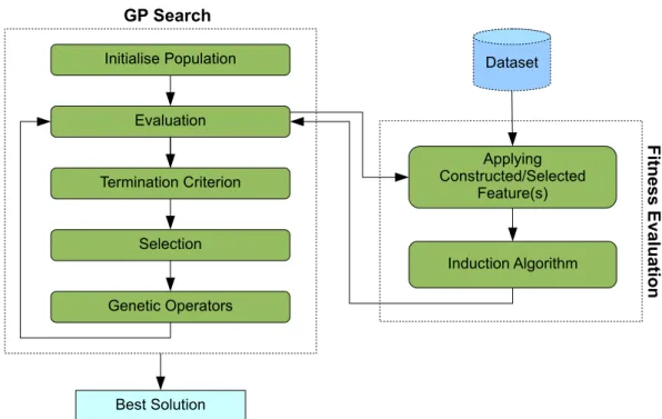
GP optimises a population of computer programs according to a fitness function that determines a program’s ability to perform a given computa-tional task [124]. The search space is explored using genetic operators [84]. Apart from the representation of genetic programs, the overall search pro-cess in GP is similar to other population-based EAs. The main steps in GP are as follows [7]:
1. Initialisea population of individual programs as solutions; 2. Assign afitnessto each individual program in the population; 3. While thetermination criterionis not met, repeat the following:
(a) Select some individuals using aselection method;
(b) Produce new individuals by applying genetic operators to se-lected members;
(c) Place new individuals into the population of the next genera-tion;
(d) Assign a fitness to each individual program in the population according to the fitness function;
4. Return the program with the highest fitness as the best solution.
2.3.3
Program Representation
Thephenotypeof each chromosome in a GP population is a program. The program is usually executed by a program interpreter. The genotype of a GP program (i.e. the way it is encoded) varies among different GP sys-tems. The most common way of encoding a GP program is through using a tree structure [19, 70]. Other common representations includeLinear GP [7, 115, 116, 52],Cartesian GP[97, 99, 98] andGrammatical GP[119, 151].
In tree-based GP, a program is represented by a hierarchy of nodes [36, 85]. Each node is either a function or a terminal[72]. Function nodes perform an operation. The children of a function node are the arguments of that function. Terminal nodes, as the name implies, do not have any children. They are either variable terminals which provide inputs to pro-grams orconstant terminalswhich are randomly generated values [7]. The set of all types of function nodes available to GP is called thefunction set. The set of all possible variable terminals is called the variable terminal set. Instrongly-typed GP, functions and terminals can have different types and the GP search must take care of building valid program trees [101, 151]. Figure 2.2 shows a sample tree-based genetic program using elementary arithmetic functions and numeric terminals.
Figure 2.2:A sample tree-based genetic program representing the mathematical expression3x2−4x+ 2. The function nodes are addition, subtraction
and multiplication. The only variable terminal node isxand constant
nodes are 2, 3 and 4.
2.3.4
Creating Initial Populations
The first step in starting a GP search is to create an initial population. The initial population is usually created randomly. There are three commonly-used ways of creating the initial population, namely theGrowmethod, the Fullmethod, and theRamped half-and-halfmethod [7].
In the Grow method, all nodes are chosen randomly, and therefore, the resulting program trees have very different shapes. To create an initial population using the Grow method, the following steps should be taken:
1. A node is randomly selected from the union of the function set and the terminal set as the root node;
2. Given n, the arity of the selected function, n functions or terminals are selected as child nodes;
3. For each child that is a function node, the previous step is repeated until the maximum tree depthis reached in which case the remaining child nodes are filled with terminals.
In the Full method, all the nodes except those at the maximum depth are functions. Therefore, the full capacity of the tree is used. The Ramped half-and-half method is used to enhance the diversity. In this method, half of the population is created using the Full method and the other half using the Grow method.
2.3.5
Genetic Operators
Genetic operators make changes to individuals in the population. They are the primary way of moving in the search space of programs. All the genetic operators work at the genotype level. Therefore, their implemen-tation highly depends on the represenimplemen-tation of GP programs [7].
2.3.5.1 Crossover
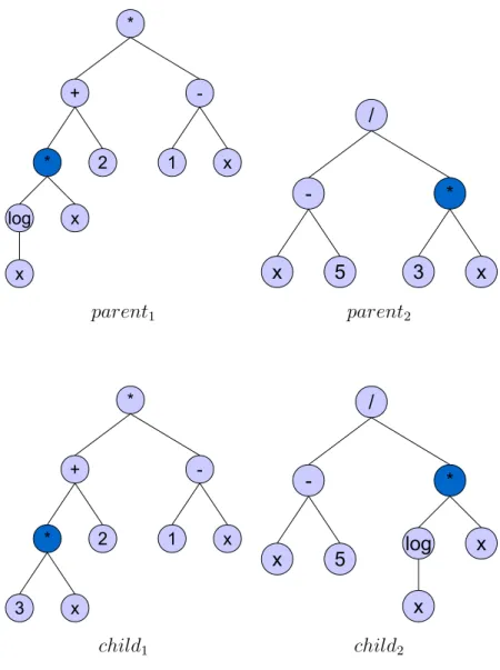
The primary function of the crossover operator is to share genetic material between individuals in the population. The crossover operator is typically applied to two individuals, calledparents, and creates two new individu-als as the result, calledchildren. In the canonical tree-based representation [71], crossover is performed by simply swapping two randomly chosen subtrees in the parent programs. Figure 2.3 demonstrate this concept with an example. To the top of the figure, there are two GP individuals. One node is randomly selected in each individual. The subtrees at these nodes are then exchanged and two new individuals are created towards the bot-tom of the figure.
parent1 parent2
child1 child2
Figure 2.3:Crossover Operator in Tree-based GP: The operator is applied to two
GP individuals, parent1 and parent2. Two nodes are randomly
se-lected and their corresponding subtrees are exchanged. The results are two new individuals,child1andchild2.
2.3.5.2 Mutation
The primary function of the mutation operator is to bring new genetic ma-terial to the population. The operator is typically applied to one individual
at a time. It performs by randomly selecting a node in the tree and then replacing the subtree at that node with a randomly-created subtree. Fig-ure 2.4 shows an example of applying the operator to a GP individual. In strongly-typed GP [101], to maintain integrity, the operation must be fai