warwick.ac.uk/lib-publications
A Thesis Submitted for the Degree of PhD at the University of Warwick
Permanent WRAP URL:
http://wrap.warwick.ac.uk/109864
Copyright and reuse:
This thesis is made available online and is protected by original copyright.
Please scroll down to view the document itself.
Please refer to the repository record for this item for information to help you to cite it.
Our policy information is available from the repository home page.
M A E G NS I T A T MOLEM U N IVER SITAS WARWICEN SIS
Evolutionary Muti-objective Worst-case Robust
Optimisation
by
Ke Lu
Thesis
Submitted to the University of Warwick for the degree of
Doctor of Philosophy
...
September 2017Contents
Acknowledgments iv Declarations v Abstract vi Chapter 1 Introduction 1 1.1 Motivation . . . 1 1.2 Research objectives . . . 3 1.3 Thesis outline . . . 3Chapter 2 Background and literature review 5 2.1 Multi-Objective Optimisation Problems . . . 5
2.2 Robust solutions . . . 6 2.3 Problem definition . . . 9 2.4 Evolutionary algorithms . . . 10 2.5 Test functions . . . 12 2.5.1 Test function 1 . . . 12 2.5.2 Test function 2 . . . 14 2.5.3 Test function 3 . . . 14 2.6 Performance measure . . . 15
2.7 A review of related work . . . 16
2.7.1 Single-objective robust optimisation . . . 17
2.7.2 Multi-objective robust optimisation . . . 18
2.7.3 Reliability . . . 21
2.7.4 Active robustness . . . 22
Chapter 3 Finding the trade-o↵ between worst-case quality and
3.1 Motivation of the developed algorithms . . . 23
3.2 Proposed solution approach . . . 26
3.2.1 The point-based nested MOEA . . . 27
3.2.2 The envelope-based nested MOEA . . . 28
3.3 Empirical evaluation . . . 35
3.3.1 Parameter settings . . . 35
3.3.2 Test results . . . 36
3.4 Summary . . . 41
Chapter 4 Improving the efficiency of bi-level worst-case optimisa-tion 42 4.1 The link to bi-level optimisation . . . 42
4.2 Background introduction . . . 43
4.3 Algorithm and New Strategies for point-based algorithm . . . 44
4.3.1 Worst case bi-level evolutionary algorithm . . . 44
4.3.2 Strategies to save fitness evaluations for point-based algorithm 45 4.4 Empirical Results for point-based algorithm . . . 48
4.4.1 Parameter settings . . . 48
4.4.2 Test results and analysis . . . 49
4.5 Test results for a given number of fitness evaluations . . . 51
4.6 Test results for the combination of three strategies . . . 54
4.7 Summary . . . 55
Chapter 5 Improving the efficiency of envelope-based algorithm 56 5.1 Motivation . . . 56
5.2 Strategies to save fitness evaluations for envelope-based algorithm . 57 5.2.1 Strategy I: Exploit upper level information for early abortion of the lower level . . . 58
5.2.2 Strategy II: Exploit the information in the neighbourhood . . 60
5.2.3 Strategy III: Skip re-evaluation if there is no improvement of the lower level front . . . 63
5.2.4 Strategy IV: Lower level smart initialisation . . . 63
5.2.5 Strategy V: Lower level generations adaptive to . . . 64
5.2.6 Strategy VI: Lower level population size adaptive to . . . 64
5.3 Empirical results for envelope-based algorithm by applying simple strategies . . . 64
5.3.1 Parameter settings . . . 65
5.4 Summary . . . 73
Chapter 6 Surrogate-assisted algorithms 75 6.1 Background and related work . . . 77
6.2 Gaussian processes . . . 78
6.3 Surrogate-assisted point-based algorithm . . . 79
6.3.1 Surrogate-assisted point-based algorithm framework . . . 79
6.3.2 Re-evaluation in surrogate-assisted point-based algorithm . . 80
6.3.3 Identity promising upper level solutions . . . 81
6.3.4 Building Gaussian process model . . . 82
6.4 Surrogate-assisted envelope-based algorithm . . . 83
6.4.1 Surrogate-Assisted envelope-based algorithm framework . . . 84
6.4.2 Re-evaluation in surrogate-assisted envelope-based algorithm 85 6.4.3 Identify “good” upper level solutions . . . 86
6.4.4 Gaussian Process model for envelope-based algorithm . . . . 87
6.5 Empirical evaluation and analysis . . . 89
6.5.1 Empirical evaluation of surrogate-assisted point-based algorithm 89 6.5.2 Empirical evaluation of surrogate-assisted envelope-based al-gorithm . . . 93
6.6 Summary . . . 94
Chapter 7 Conclusion and future work 97 7.1 Research summary . . . 97
7.2 Contributions . . . 98
7.3 Limitations . . . 101
7.4 Future research work . . . 102
Acknowledgments
I would like to express my foremost appreciation to Professor Juergen Branke for his continuous support, great patience, wise advise, encouragement throughout my PhD study and related research at Warwick Business School. I could not have imagined having a better supervisor to supervise my PhD study. His invaluable insights and guidance helped me accomplish the thesis.
I would also like to take this opportunity to thank Professor Tapabrata Ray, for all his valuable comments and suggestions. I also thank my second supervisor Nalan Gulpinar for her encouragement.
Last but not least, I would like to thank my family. Especially my mother who always supports me and encourages me over my PhD study. In my first year of the PhD study, I was depressed and everything seemed hopeless. It was my mother who encouraged me to continue my study. Because of their unconditional support, I have the determination to finish my study.
Declarations
This thesis is submitted to the University of Warwick in support of my application for the degree of Doctor of Philosophy. It has been composed by myself and has not been submitted in any previous application for any degree. The work presented was carried out by the author.
Parts of this thesis have been published by the author:
• Juergen Branke and Ke Lu. Finding the trade-o↵ between robustness and worst-case quality. In Proceedings of the 2015 Annual Conference on Genetic and Evolutionary Computation, pages 623-630. ACM, 2015.
• Ke Lu, Juergen Branke, and Tapabrata Ray. Improving efficiency of bi-level worst case optimization. In International Conference on Parallel Problem Solving from Nature, pages 410-420. Springer, 2016.
Abstract
Many real-world problems are subject to uncertainty, and often solutions should not only be good, but also robust against environmental disturbances or de-viations from the decision variables. While most papers dealing with robustness aim at finding solutions with a highexpectedperformance given a distribution of the un-certainty, we examine the trade-o↵between the allowed deviations from the decision variables (tolerance level), and the worst case performance given the allowed devia-tions. In this research work, we suggest two multi-objective evolutionary algorithms to compute the available trade-o↵s between allowed tolerance level and worst-case quality of the solutions, and the tolerance level is defined as robustness which could also be the variations from parameters. Both algorithms are 2-level nested algo-rithms. While the first algorithm is point-based in the sense that the lower level computes a point of worst case for each upper level solution, the second algorithm is envelope-based, in the sense that the lower level computes a whole trade-o↵curve between worst-case fitness and tolerance level for each upper level solution.
Our problem can be considered as a special case of bi-level optimisation, which is computationally expensive, because each upper level solution is evaluated by calling a lower level optimiser. We propose and compare several strategies to improve the efficiency of both algorithms. Later, we also suggest surrogate-assisted algorithms to accelerate both algorithms.
Chapter 1
Introduction
1.1
Motivation
Many real-world optimisation problems are subject to uncertainties that are prac-tically impossible to avoid. For instance, in manufacturing, it is usually impossible to produce an item exactly following the design specifications as shown Figure 1.1, there are always some manufacturing tolerances. The solutions could be potentially risky to use if uncertainties have not been taken into account during optimisation. Hence, when solving real-world optimisation problems, it is important to consider solutions that are not only globally optimal but also practical to use in reality despite the di↵erent uncertainties present within those problems. In other words, people prefer solutions that not only have good quality but also have tolerance against uncertainties.
One extensively used concept of robustness for single-objectiveoptimisation is proposed by Branke (1998). The objective function is replaced by its mean function, for any solutionx, it maps to its average function value in a pre-defined neighbour-hood ofx. The mean function is minimised instead of the objective function. Those
solutions whose function values in the neighbourhood does not change much are considered as good.
Two concepts of robustness for multi-objective optimisation are introduced in Deb & Gupta (2006). The first one replaces the objective functions by the mean functions as Branke (1998) for a single objective function. Robust solutions are defined as the efficient solutions obtained by optimising the mean functions. The second concept optimises the original objective functions with the constraints that does not allows the variations between the objective function values and the mean function values to be greater than a certain limit. The second concept gives the users an option to define the level of robustness. Our approach also allows the user to make decisions with di↵erent robustness levels. The di↵erence is that we look at the worst-case fitness, and get a trade-o↵ between worst-case fitness and robustness. In the second concept, the optimal solutions are based on a single pre-defined robustness level, for di↵erent robustness levels, the problem is solved more times.
The first concept in Deb & Gupta (2006) is extended in Barrico & Antunes (2006) by introducing the degree of robustness if a solution. A feasible solution has a predefined neighbourhood, and it measures how much this neighbourhood can be extended with the constraints that the variations between the objective functions values and the mean function values can not be larger than a predefined limit.
Gunawan & Azarm (2005) introduce sensitivity region with uncertainty in the parameters space to measure the robustness in multi-objective optimisation problems. The allowed variations of the parameters is defined as the sensitivity region by restricting the variations of the objective function values within a certain limit. They also introduce worst-case-sensitivity region because the sensitivity re-gion could not be asymmetric. This worst-case rere-gion fits into the sensitivity rere-gion with a maximum radius.
Avigad & Branke (2008) propose an evolutionary algorithm to search for solutions in a multi-objective optimisation problem with uncertainty in the design and parameter space. Each nominal solution corresponds to a worst set of sce-narios. The algorithm aims to search for solutions that have the best worst-case performance.
In this thesis, we will look at the uncertainty in decision space. On the one hand, we look at the quality of a solution. On the other hand, its good tolerance against uncertainty will be desired. The aim is to deal with the uncertainty and search for robust solutions for a given tolerance level. There will be more than one criterion to consider (solution quality and good tolerance against uncertainty).
Risk averse decision makers may care about the worst-case performance with decision variables disturbed by uncertainty. If the worst-case situation involves po-tential bankruptcy, death or system breakdown, it is of great importance to look at the worst-case quality. For a solution with a certain tolerance level, the worst-case performance will be considered. A possible application are manufacturing toler-ances, where an engineer can specify an allowed tolerance for manufacturing. A low tolerance requirement incurs substantially higher manufacturing cost, whereas a high tolerance usually means having to accept a lower worst-case quality of the solution. We address the uncertainty in the decision space, and a solution with good worst-case performance is considered as robust against uncertainty. We attempt to search for the trade-o↵between worst-case quality and tolerance levels. The trade-o↵ would provide information to decision makers so that they can make informed decisions with respect to personal preferences.
1.2
Research objectives
For an optimisation problem with uncertainty in the decision space, solutions that not only have good quality but also have good robustness are preferred. We will look at how uncertainty is modelled within the problems and define robust solutions and robustness. In this research, we consider the worst-case performance if disturbed by uncertainty in the decision space. We would like to study a trade-o↵ between the worst-case performance and robustness. This research seeks to achieve the following objectives.
1. Propose a formal framework which defines the formulations of the worst-case performance and robustness.
2. Develop algorithms to search for the trade-o↵between worst-case quality and robustness.
3. Improve the efficiency of the developed algorithms.
1.3
Thesis outline
The overall structure of the thesis takes the form of seven chapters.
Chapter 2 provides a brief description of the multi-objective optimisation problem and defines the problem framework of this research. For multi-objective optimisation problems, the optimal solutions are a set of non-dominated solutions with di↵erent trade-o↵s. Because we investigate uncertainty in the decision space,
the robust solutions are described. Robustness in our thesis is defined as the maximal allowed deviation from the decision variables. The problem we solve is explained and formulated in the problem definition. What follows is a set of test functions that are used to test our algorithms and methods proposed in the following chapters. The performance measure Inverted Generational Distance is applied to evaluate the quality of the Pareto optimal solutions obtained by each algorithm. The final section discusses related work in robust optimisation.
In Chapter 3, two newly developed algorithms are suggested to solve the problem described in Chapter 2. The first algorithm is point-based in the sense that the lower level is a single objective optimisation problem that returns a single value to the upper level. The second algorithm is envelope-based because the lower level is a multi-objective optimisation problem which returns a set of solutions with di↵erent trade-o↵s (envelope) to the upper level.
Both algorithms in Chapter 3 are bi-level which is computationally expensive, because each upper level solution is evaluated by calling a lower level optimiser that, in our case, is population based. Therefore, in Chapter 4, we propose and compare several strategies to reduce the computational costs of the point-based algorithm. The aim of this chapter is to obtain a reasonably good Pareto front at upper level given a small number of fitness evaluations. Chapter 5 extends the strategies to the envelope-based algorithm.
In Chapter 6, we combine our algorithms with surrogate models in order to accelerate the algorithms. Generally, a surrogate model is built to approximate the actual objective function values. In our case, we would like to apply surrogate models to learn the robust function rather than actual fitness. The surrogate model is used to identify those solutions are promising in the upper level, and only the good solutions are evaluated by running the lower level algorithm.
Chapter 7 concludes the thesis with a summary of the contributions and limitations, as well as some ideas for future work.
Chapter 2
Background and literature
review
Considering decision variables disturbed by uncertainty, we often prefer solutions that are not only good, but also robust against environmental disturbances or devi-ations from the decision variables. While most papers dealing with uncertainty in the decision space aim to find solutions with a high expected performance given a distribution of the uncertainty, we examine the trade-o↵between the allowed devi-ations from the decision variables (tolerance level), and the worst case performance given the allowed deviations.
2.1
Multi-Objective Optimisation Problems
Assuming maximisation without loss of generality, the multi-objective optimisation problems (MOPs) could be defined as follows:
max f(x) =f1(x), f2(x), ..., fm(x) (2.1)
s. t.
g(x)0 (2.2)
h(x) = 0 (2.3)
wheref(x) is the objective function vector to be optimised that consists ofm
objectives, andg(x) andh(x) are the inequality constraints and equality constraints, respectively.
value is uniquely defined. However, when there is more than one objectives to be optimised, the optimal solutions are likely to consist of a set of alternative trade-o↵s. We now define the basic terminology as follows.
• Pareto Dominance
Without loss of generality, for a multi-objective maximisation problem, the Pareto dominance relationship can be described as follows:
A solution vector x is said to dominate another y if fi(x) fi(y) for all objectives, andfi(x)> fi(y) for at least onei.
• Pareto Optimal Solution Set
A solutionxto the problem is defined as Pareto optimal if it is not dominated by any other feasible solutiony.
• Pareto Front
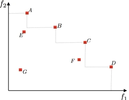
The image of all Pareto optimal solutions in the objective space is known as Pareto front, and it is also known as efficient front. Figure 2.1 shows the dominance relationship for a two objectives maximisation problem, where
f1 and f2 are the two objectives to be maximised. Solutions A-D are
non-dominated solutions that form the Pareto front. Solution E is non-dominated by A and B, and Solution F is dominated by C. Solution G is dominated by all other solutions.
2.2
Robust solutions
In this section, we describe robust solutions with uncertainty in decision space and introduce the robustness definition.
1. Uncertainty in decision space
With uncertainty in the decision space, the objective function can be expressed as:
f(x+ ) (2.4)
where is the uncertainty vector in decision variables. Usually is restricted within a specified range or follows a known distribution.
Figure 2.1: An example of Pareto dominance relationship between two objectives to be maximised
There are several robustness definitions. If a solution has tolerance against uncertainty in the decision space, we say this solution is robust and has good tolerance. In our research, the robustness is defined as the allowed deviation from the decision variables which is also called as tolerance level.
3. Robust solutions
Typically, evolutionary algorithms aim to find a globally optimal solution. However, if such a solution is very sensitive to small variations of the decision variables or operating environment, in practice, people may prefer solutions that have perhaps slightly inferior quality but also have good tolerance to uncertainty. There are a number of di↵erent definitions for robust solutions (Branke 2001), including having a good expected performance and a good worst-case performance. Generally, a robust solution is defined as a solution whose fitness is not sensitive to small variations in decision space or environ-ment. If a solution has good tolerance to small variations of decision variables, we say this solution has good tolerance against uncertainty.
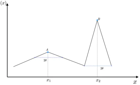
From Figure 2.2, if two solutionsAandB are disturbed by uncertainty that is bounded to [ ✓,✓], the solution quality ofB in terms off varies much more thanA. SolutionA is less sensitive to uncertainty and more robust thanB. If we consider the expected value of the objective function within the
distur-Figure 2.2: An example function used for description of robust solutions bance region,
fE(x) =
Z
p( )f(x+ )d
wherep( ) is the probability density function of . We would like to maximise the expected value
max
x f
E(x)
If we look at the worst-case value in the disturbance region,
fw(x) = minf(x+ )
where 2[ , ], and is the maximal disturbance for x.
We would like to maximise the worst-case value max
x f
w(x)
In our research, we consider the worst-case quality in the disturbance region. Usually, for a solution as its tolerance level increases, the worst-case quality within the disturbance region will drop. Solutions with greater tolerance level and better worst-case fitness are preferred. As shown in Figure 2.2, the decision variable may be disturbed by belongs to the range [ ✓,✓], solution A has
better worst-case quality thanB.
2.3
Problem definition
We assume that an objective functionf(x) and an allowable range forx2[xmin, xmax]
are given. The optimisation is not only overx, but the user can also set a tolerance level , and the goal is to identify the trade-o↵between tolerance level and worst case performance within the tolerance region [x , x+ ], which we assume to be symmetric around x. Without loss of generality assuming a maximisation prob-lem here, the two objectives we want to maximise are fw(x, ) = miny{f(y)|y 2
[x , x+ ]}and .
To summarise, the aim is to identify all Pareto optimal solutions for the following 2-objective optimisation problem:
max fw(x, ) (2.5)
max (2.6)
s. t.
x2 [xmin, xmax] (2.7)
2 [0,min{x xmin, xmax x}] (2.8)
Equation 2.8 ensures that the tolerance region can not exceed the allowed search space (i.e., a solution at the border of the feasible space can not have a tolerance lever greater than zero). Note that this is a nested optimisation problem, as the calculation offw(x, ) = min
y{f(y)|y 2[x , x+ ]}is itself an optimisation problem.
Because the space forx is bounded, the maximal possible tolerance level of a solutionx is bounded by how far away x is from the boundary. As a result, the feasible space is a triangle and is shown in Figure 2.3 for a one dimensional problem. For a univariate problem, it can be represented by the framework described above straightforward. We give the representation of a two-dimensional problem
f(x1, x2) withx1 and x2,x= (x1, x2), where
x12[xmin1 , xmax1 ]
Figure 2.3: The feasible search space
For these two variables, the robustness for each variable is restricted to
12[0,min{x1 xmin1 , xmax1 x1}] 22[0,min{x2 xmin2 , xmax2 x2}]
We can get that the robustness is bounded to [0,min{ 1, 2}]. The
worst-case fitness calculation is displayed as
fw(x1, x2, ) = min
y1,y2{
f(y1, y2)|y1 2[x1 , x1+ ], y22[x2 , x2+ ]}
The problem is formulated as a multi-objective optimisation problem where the two objectives worst-case quality and robustness are optimised. The optimal solutions to this problem will be a set of non-dominated solutions. We would like to develop algorithms to search for the trade-o↵ between worst-case quality and robustness. This will provide information to help the decision maker. For a certain robustness, the best worst-case performance can be identified from the trade-o↵.
Evolutionary Algorithms (EAs) are able to search for a set of near-optimal solutions with di↵erent trade-o↵s at the end of an optimisation procedure.The main techniques applied in this research are based on multi-objective EAs.
2.4
Evolutionary algorithms
EAs have been extensively used to deal with complex optimisation problems (Coello et al. 2007). EAs are stochastic optimisation methods derived from natural evolu-tion: given a randomly initialised population of individuals in the search space, these individuals evolve with respect to the Darwinian principle of the survival of the fittest. The fitness of the population increases with the evolution. Without
loss of generality, given an objective function to be maximised, randomly generate a set of candidate solutions, each solution is evaluated in terms of its fitness. The fitness function measures how well the solutions perform. The solution with higher fitness is considered better. Based on the fitness evaluations, some of the solutions in the population are selected to survive to the next generation. The probability of survival of the new individual depends on their fitness: the individuals with a high fitness are more likely to be kept while individuals with low fitness would be discarded.
Three major evolutionary operators are mutation, recombination and/or se-lection, and they are applied to generate new solutions. Recombination is used to produce one or more new solutions by selection two or more solutions in the popu-lation. Mutation is applied to one solution to create a new solution. The o↵spring population that is the newly generated solutions by recombination and mutation. Each solution in the o↵spring population is evaluated based on its fitness. The so-lutions in both population and o↵spring compete in terms of the fitness, and select a number of better solutions that survive to the next generation. This describes one iteration of the evolution, and this process evolves until the optimal solutions are obtained or the stopping condition is satisfied.
The flowchart of EAs could be expressed as Figure 2.4, which describes the process of EAs (Eiben et al. 2003). They summarise the evolutionary operators as follow:
• Variation operators that contains recombination and mutation, and they are applied to create new solutions in the population.
• Selection operator drives the improvement of the solutions quality in the pop-ulation.
In some variants of evolutionary algorithms selection is deterministic, always selecting the best individual. While the selection could be probabilistic, and the best individuals are not selected deterministically.
The general evolutionary algorithm is described as initially generate a set of candidate solutions randomly that form the parent population, and evaluate each solution in the parent population. Repeat the following process until the stopping condition is satisfied. Select solutions from the parent population, recombine the selected solutions to generate o↵springs and mutate the o↵springs to get the o↵spring population. Evaluate each new solution in the o↵spring population, select good individuals from the combined parent and o↵spring population that goes to the next generation. A population whose quality is getting better as the EA evolves.
Figure 2.4: The flow chart of a standard EA
One of the main advantages of evolutionary algorithms is that all they need is the objective function and fitness measures about the optimisation problem. They can deal with constrained or unconstrained non-linear problems that are defined in discrete or continuous search spaces. Besides, the evolutionary algorithms search for the optimal solutions in the whole search space and this makes them global.
2.5
Test functions
2.5.1 Test function 1
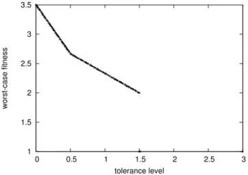
We propose the following simple one-dimensional functionf(x), which is visualised in Figure 2.5: f(x) = 8 > > > > > > > < > > > > > > > : 5 3x 2 3 if 1< x 5 2 5 3x+ 23 3 if 5 2 x4 2 3x 2 3 if 4< x 11 2 2 3x+ 20 3 if 11 2 < x7
1 1.5 2 2.5 3 3.5 1 2 3 4 5 6 7 f(X) X 1 1.5 2 2.5 3 3.5 0 0.5 1 1.5 2 2.5 3 worst-case fitness tolerance level ’truef1’
Figure 2.5: The plots of test function 1 (left) and its true Pareto front (right) The function has two peaks. The corresponding true (fw, ) Pareto front can be derived as follows. The solution with the best worst-case fitness is clearly the solution at the highest peak (x = 2.5) with tolerance level = 0. As the tolerance level is increased up to = 0.5, the solution x= 3.5 remains the optimal solution, but the worst case obviously degrades down to 8/3. If greater tolerance levels are desired, it is better to switch to solution x = 5.5. Although the peak is lower, it is also not as steep, which yields a better worst-case performance for larger tolerance regions. At = 1.5, there is no solution that would not havex= 4 within its tolerance region [x , x+ ], and thus the worst case fitness drops to
f(4) = 1. If this worst case is accepted, can be increased to 3 by choosing x= 4, which is the maximally robust solution. So, the Pareto set consists of all solutions (x = 2.5, 2 [0,0.5]),(x = 5.5, 2 (0.5,1.5)),(x = 4, = 3). The two objectives we would like to optimise are the worst-case fitness and robustness, for this simple test function, we can derive the relationship between those two objectives and can be defined mathematically as fw( ) = max
x (f
w(x, )). For each decision variable, search for the best worst-case fitness with di↵erent tolerance levels. The trade-o↵
between those two objectives is depicted in Figure 2.5. For each robustness, we can calculate the corresponding best worst-case fitness. Therefore, the trade-o↵between the worst-case fitness and robustness can be represented byfw( ) as follow:
fw( ) = 8 > > > < > > > : 5 3 + 3.5 if0 0.5 2 3 + 3.0 if0.5< <1.5 1.0 if = 3.0
0 0.5 1 1.5 2 2.5 3 3.5 0 2 4 6 8 10 f(X) X 0 0.5 1 1.5 2 2.5 3 3.5 0 1 2 3 4 5 worst-case fitness tolerance level ’truef2’
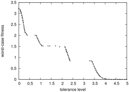
Figure 2.6: The plots of test function 2 (left) and its approximated true Pareto front (right)
2.5.2 Test function 2
The following test function has been taken from Lim et al. (2005), and a plot of this function is shown in Figure 2.6. It has more local optima which makes it more interesting. The true Pareto front shown in Figure 2.6 is approximated by generating a number of equally distributed samples , and then for each find its optimal worst-case fitness by sampling a number of upper level input designsxi.
f(x) = 2e (x 2)2/0.32+ 2.2e (x 3)2/0.18+ 2.4e (x 4)2/0.5
+2.3e (x 5.5)2/0.5+ 3.2e (x 7)2/0.18+ 1.2e (x 8)2/0.18
where 0x10.
2.5.3 Test function 3
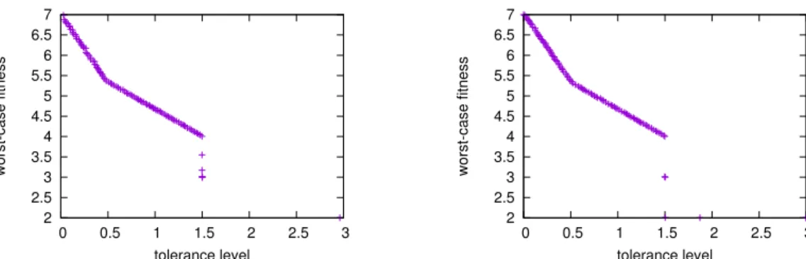
This is simply a 2-dimensional version of test function 1, and defined as f(X) =
P
f(xi). It is visualised in Figure 2.7. The function has four peaks, which are
f(2.5,2.5) = 7.0,f(2.5,5.5) = 6.5,f(5.5,2.5) = 6.5,f(5.5,5.5) = 6.0. Its worst-case fitness and robustness have beed described in the problem definition.
Its true Pareto front (fw, ) can be derived as follows. The solution with the best worst-case fitness is the solution at the highest peak (x1 = 2.5, x2 = 2.5)
with tolerance level = 0. With the tolerance level increased up to = 0.5, the solution (x1 = 2.5, x2 = 2.5) remains the optimal solution, while its
worst-case fitness drops to 16/3. If the tolerance level continues to increase, the optimal solution will be (x1 = 5.5, x2= 5.5) that has the lowest peak. The solution with the
1 2 3 4 5 6 7 1 2 3 4 5 6 7 2 2.5 3 3.5 4 4.5 5 5.5 6 6.5 7 f(X) x1 x2 f(X) 2 3 4 5 6 7 0 0.5 1 1.5 2 2.5 3 worst-case fitness tolerance level ’truef3’
Figure 2.7: The plots of test function 3 (left) and its true Pareto front (right) fitness for higher tolerance levels. When the tolerance level goes up to = 1.5, for each solution can have this tolerance level, its region always include the solution (x1 = 4.0, x2= 4.0), and its worst-case fitness will degrade tof(4.0,4.0) = 2.0. As
increased to the maximum tolerance level 3.0 with the solution (x1 = 4.0, x2 = 4.0),
the corresponding worst-case fitness stays at 2.0. Therefore, the true Pareto optimal solution set will be (x1 = 2.5, x2 = 2.5, 2 [0,0.5]), (x1 = 5.5, x2 = 5.5, 2
(0.5,1.5)), and (x1 = 4.0, x2 = 4.0, = 3.0). So we can get its true Pareto front
shown as Figure 2.7. fw( ) = 8 > > > < > > > : 10 3 + 7.0 if0 0.5 4 3 + 6.0 if0.5< <1.5 2.0 if = 3.0
2.6
Performance measure
The most widely used performance metric for multi-objective optimisation is proba-bly the Hypervolume (Zitzler & Thiele 1998), which measures the volume bounded by a reference point and non-dominated solutions in the objective space. However, in our case, the proposed algorithms may find solutions on either side of the true Pareto front. If the lower level EA does not properly identify the worst case, then the information provided to the upper level EA is too optimistic, individuals will appear better than they are, and solutions to the upper right of the true Pareto front may appear (they do not actually exist, but the algorithm reports them as solution). On the other hand, even if the lower level EA computes the correct worst case, the upper level may not be able to find the best upper level solutions, in which case
the results will appear towards the lower left of the true Pareto front. Hypervolume would count the former error (solutions perceived as too good) as benefit, and is thus not really suitable.
We therefore propose to use the inverted generational distance (IGD) met-ric (Knowles & Corne 2002). This metmet-ric requires a number of targets along the true Pareto front, and then sums up the distances between each target and the closest point in the Pareto front approximation identified by the algorithm. We have chosen 100 equidistant points along the true Pareto front as targets. Because IGD tends to be smaller if the number of solutions in the Pareto front approximation is larger, and our two algorithm variants have di↵erent population sizes, we used crowding distance pruning to reduce the number of solutions returned by each algorithm to 100 before computing the IGD metric. For each point, its nearest neighbours in the same front define a cuboid and a crowding distance metric is defined as the average side length of this cuboid. This metric is used in the selection to keep the population diverse, because the larger this metric value, the fewer points in the neighbourhood of this point. Crowding distance pruning means to use the crowding distance as the selection criteria to remove solutions in the population gradually.
2.7
A review of related work
A number of papers (Beyer & Sendho↵2007, Jin & Branke 2005, Roy 2010, Gaspar-Cunha & Covas 2006, 2008, Bertsimas et al. 2011, 2010) have suggested to use evo-lutionary algorithms (EAs) to search for robust solutions in optimisation problems. Uncertainties in optimisation problems have been addressed in many application areas (Ide et al. 2015) (Gu et al. 2013) (Thompson 1998) (Greiner 1996) (Wies-mann et al. 1998) (Anthony & Keane 2003a) (Anthony & Keane 2003b) (Chen et al. 2012) (Sebald & Schlenzig 1994). Jin & Branke (2005) provide a survey on evo-lutionary optimisation with uncertainty. Uncertainty in evoevo-lutionary computation is divided into four categories: 1) The fitness function is subject to noise that is often assumed to follow a normal distribution with mean zero and variance 2. The expected fitness function is often approximated by an averaged sum of a number of random samples. 2) The decision variables or environmental parameters are per-turbed. Solutions that still work well with slight variations in decision variables are defined as robust solutions. Those solutions are desired rather than global optimal solutions. 3) If the fitness function is approximated it su↵ers from approximation errors. 4) The fitness function changes over time. Beyer & Sendho↵(2007) makes a survey of robust optimisation. They discusses how to address di↵erent kinds of
uncertainties and how to evaluate robust solutions. Ide & Sch¨obel (2016) introduce a variety of robustness concepts for multi-objective optimisation problems with un-certainty. Goh & Tan (2007b) and Beyer (2000) examine evolutionary optimisation with noisy environments.
A considerable amount of literature has been published on optimisation prob-lems with uncertainty. The previous studies will be discussed in the following sec-tions. The first section reviews single-objective robust optimisation. The second section focuses on multi-objective robust optimisation. The third section will dis-cuss optimisation problems with uncertainty in the constraints. Finally, it introduces active robustness where a parameter can be adjusted to mitigate the disturbance.
2.7.1 Single-objective robust optimisation
Most of the papers to date search for solutions with a good expected performance given a distribution of possible disturbances of the decision variables. The main challenge then is to estimate the expected performance efficiently. One of the ear-liest approaches was probably (Tsutsui & Ghosh 1997, Tsutsui et al. 1996, Tsutsui 1999, Tsutsui & Ghosh 2003) who suggested to simply disturb the decision variables randomly before evaluation. They show that for the limit case of infinite population sizes, this would lead the EA to search the landscape of expected fitness. To get more accurate estimates of the expected fitness also with small population sizes, researchers have proposed explicit averaging over multiple samples (e.g., (Branke 1998, Wiesmann et al. 1998, Branke 2001)) or also to use surrogate functions to avoid costly fitness function evaluations (Paenke et al. 2006). Branke & Schmidt (2005) introduce two fitness estimation methods that are interpolation and regres-sion. Forouraghi (2000) optimises a “signal-to-noise ratio” rather than the expected fitness, which is basically a mean of squared fitness values, penalising variance. In-terestingly, Forouraghi (2000) does not pre-specify the distribution of disturbances, but assumes equal distribution in an area that can also be set by the EA. So, the EA specifies a range for each decision variable, rather than a single value.
Beyer & Sendho↵(2006) address optimisation with actuator noise where the noise is added to the design variables. The expected value robustness measure is optimised, and Evolution Strategies (ESs) are suggested to solve the problem where the mutations in ESs play the role of robustness tester.
2.7.2 Multi-objective robust optimisation
While most of the work on EAs for searching robust solutions assumes a single objective function, there are few papers that transfer these concepts to the multi-objective case (Deb & Gupta 2005, 2006, Forouraghi 2000, Saha et al. 2011). Some authors have also used multi-objective evolutionary algorithms (MOEAs) to ex-amine the possible trade-o↵ between solution quality and robustness, again with various definitions of robustness. In addition to the nominal (undisturbed) perfor-mance of a solution, Jin & Sendho↵ (2003) consider a variance measure, Luo & Zheng (2008) consider an estimate of the gradient in the neighbourhood, and Goh & Tan (2007a) consider the maximum percentage degradation in fitness within a given neighbourhood. They present a robust multi-objective evolutionary algorithm (RMOEA) that aims to evolve the trade-o↵between Pareto optimality and robust-ness. They consider the worst-case scenario for each candidate solution and use local search process to find its worst performance. The way they measure the robustness is fi0(x) = max(fi(x
0) f
i(x))
fi(x)
that describes the variation degree arising from the worst objective value. In our problem, the robustness is defined as the maximum allowed deviations from the decision variables. We get the actual worst-case fitness with no variation degree constraint.
In (Li et al. 2005, Lim et al. 2005, 2007), robustness is considered as the maximum deviation from the specified decision variables that guarantees that the drop in performance from nominal to realised fitness is no more than some pre-specified threshold. Deb et al. (2009) look at the trade-o↵between performance and reliability, which is the probability of the solution being feasible.
Deb & Gupta (2005) suggest methods that search for robust solutions in multi-objective optimisation problems. The aim is to find solutions that are less sensitive to small changes in variables. Two di↵erent robust multi-objective op-timisation procedures are presented to find the robust optimal front rather than the global Pareto-optimal front. They optimise the mean e↵ective objective val-ues that are computed by averaging the objective function valval-ues of solutions, in-stead of the original objective functions. They define two types of multi-objective robust solutions. In type I, the mean e↵ective objective values are defined as
fjef f(x) = 1
|B |
Z
y2x+B
fj(y)dy, where |B | is the volume of the neighbourhood. In type II, they optimise the original objective function by setting the constraints
kfp(x) f(x)k
kf(x)k ⌘. f
p(x) can be the mean e↵ective function value or the worst function value in the vicinity. This means the variations of objective values should be no more than a certain percentage of the original objective function value of a
solution with respect to the pre-defined⌘. The single-objective robust optimisation problems (SROPs) are extended to multi-objective robust optimisation problems (MROPs) by evaluating the e↵ective objective functions, and the technique is de-noted as E↵-MOEA.
Lee & Park (2001) take into account uncertainty in form of variations from the decision variables in engineering optimisation problems. Assume the disturbed decision variable is normally distributed with the meanµxi and standard deviation
xi. The tolerance band of this decision variable is defined as a⇤ xi. If a = 3,
99.73% of the decision variable exists within [µxi 3 xi, µxi+ 3 xi]. This is similar
to the tolerance level is our problem, but our decision variables are bounded to an allowable range.
Jin & Sendho↵ (2003) consider the robustness as an additional objective and the single objective optimisation problem becomes a multi-objective optimisa-tion problem. A trade-o↵ between the performance and robustness is considered. Gunawan & Azarm (2005) introduced sensitivity region concept to measure the multi-objective sensitivity of a design. Considering the objective function contains design variables and parameters, if the variations in objective value is small when the parameter changes, then the design variable is not sensitive to parameter variations. It does not require the parameter distribution so this methods also applies to objec-tive functions that are non-di↵erentiable or discontinuous. Li et al. (2005) describe the robust optimal solutions are those solutions that are less sensitive to parame-ter variations, if the multi-objective optimisation problems involve parameparame-ters that are uncontrollable. A new Robust Multi-Objective Genetic Algorithm (RMOGA) is presented in (Forouraghi 2000) to get the trade-o↵ between performance and a robustness index that is defined based on worst-case sensitive region. Luo & Zheng (2008) propose a new method to search for robust solutions by converting a multi-objective robust optimisation problem into a bi-multi-objective optimisation problem, one objective represents the solutions’ quality and the other objective is to optimise the solutions’s robustness.
For multi-objective optimisation problems in the presence of uncertainty, a conservative method to tackle them is to search for a solution that is robust with respect to best worst-case performance in all possible scenarios. Vasile (2014) search for the optimal design in worst-case scenario as robust solutions. There are also some papers solving minmax problems using coevolutionary algorithms (Jensen 2004) (Jensen 2001) (Branke & Rosenbusch 2008). Evidence-based robust optimisation is introduced in (Alicino & Vasile 2014) to solve multi-objective minmax problems. In (Marzat et al. 2013), Kringing and relaxation is combined to deal with
worst-case global optimisation of black-box functions. Herrmann (1999) aims to solve minmax optimisation problems and find robust solutions that have best worst-case performance with respect to di↵erent scenarios.
Inverse multi-objective robust evolutionary (IMORE) design optimisation with uncertainty is proposed by Lim et al. (2005). They consider the worst-case performance for a given performance degradation leveldt. There are two criteria to be optimised, one is nominal fitness and the other is robustness that is defined as the maximum variations for decision variables that allow the performance degradation no larger than the permitted degradation tolerancedt. Based on those two criteria they search for the trade-o↵ between the nominal fitness and robustness. IMORE is a three-level algorithm, for any decision variable in the first level, the third level returns the worst-case performance and the second level returns the robustness.
Avigad et al. (2005) treats the robustness as the result of delayed decisions for the conceptual design, and a robust non-dominance sorting procedure is involved. Considering uncertainty in multi-objective optimisation problems, the performances of solutions depend on di↵erent scenarios. Later, Avigad & Branke (2008) extend the worst-case evolutionary multi-objective optimisation where the number of scenarios is larger, such that for each solution the worst cases will be a set. Branke et al. (2013) introduces Pareto dominance concept to worst-case optimisation problems, where the authors extended the dominance relation to each solution is presented by a set of fitness vector. Two approaches, the expected marginal utility and an indicator based on (Zitzler et al. 2003), are proposed to rank individuals within a front.
(Kuroiwa & Lee 2012) use the worst-case approaches and define three robust solutions for the multi-objective optimisation problem. For each objective function, its worst-case over all scenarios is considered. The uncertain multi-objective op-timisation problem will become deterministic by optimising the worst-case of each objective, and the efficient solutions are defined as robust. Barrico & Antunes (2006) applied a degree of robustness concept that is similar to (Lim et al. 2005) to search for robust solutions. For a pre-defined threshold of objective variations, the de-gree of robustness of a solution is defined as the maximum radius inside a hyper box around it. (Meneghini et al. 2016) propose a coevolutionary algorithm to solve robust multi-objective optimisation problems. They use two populations that rep-resent the solutions and uncertainties, respectively. These two populations compete in the environment.
2.7.3 Reliability
For an optimisation problem with uncertainty in both objective function and con-straints, an optimal solution may become infeasible due to the uncertainty. A solu-tion with a small probability of becoming an infeasible is considered as more reliable. The di↵erence between reliability and robustness is that reliability focuses on solv-ing the constraints to make the solution feasible. There are also some papers that consider the uncertainty in constraints. Deb et al. (2009) consider the reliability of solutions. A solution is considered as reliable if it is robust in terms of feasibility with the uncertainty in the decision variables. Ray (2002) pointed out that it is of no practical use to maximise the performance only, because a solution may be too sensitive to small variations. The author proposed to use EAs to maximise three objectives that include a solution’s performance, its mean and standard deviation in the neighbourhood. Gupta & Deb (2005) investigate constraints handling in robust multi-objective optimisation.
Deb & Gupta (2006) investigate the two notions in more detail, and they extend them to constrained optimisation problems. They introduce the index ro-bust constraint violation of each solution: RCV(x) = Py2B (x)CV(y), and the constraint violation of y is defined as CV(y) = Pj < gj(y) >. The bracket op-erator < > is defined as Pjmin{gj(y),0}. This means that any point in the neighbourhood of a solution violates any constraint, this solution will be considered as infeasible. An index of robust constraint violation of each solution is defined as the the sum of the constraint violations of solutions in the neighbourhood of the candidate solution.
In (Goh & Tan 2007a), the µGA optimises a multi-objective problem that maximises the worst case objective and the worst constraint violation, and the second criterion also considers the feasibility. Moreover, the memory-based feature of tabu search (TS) is implemented to improve computational efficiency, while the constraints under uncertainty and periodic re-evaluation of archived solutions are used to reduce uncertainty of evolved solutions. Lee & Park (2001) also consider the robustness of constraint functions that is the feasibility of the constraints. A penalty factor is included to control the robustness of the constraint function. On the one hand, the increase of the penalty factor will decrease the possibility that a solution enters into the infeasible region. On the other hand, the objective function value will become worse with the increase of the penalty factor.
2.7.4 Active robustness
The robust optimisation tries to find robust solutions where the decision variable is fixed and the robustness is inherent within the solutions. This kind of robust-ness is passive. The active robustrobust-ness is introduced in (Salomon et al. 2014). They consider problems that contain uncertain environmental parameters and adjustable variables that can be modified after the environmental parameters have been re-vealed (Salomon et al. 2013). For each candidate solution, its performance changes according to the scenario of environment and adjustable variable. Therefore when the environment changes, solutions’ performance and robustness can be improved by adaptation. There are two objectives considered, one is the performance and the other is the cost of adaptation. They combine robust and dynamic optimisa-tion to form active robust optimisaoptimisa-tion. However, they do not consider the cost of adaptation. In (Salomon et al. 2015), the active robust optimisation problem is extended to multi-objective optimisation problems. They consider the active robust optimisation problem as a bi-level optimisation problem. The di↵erence is that the lower level searches for the optimal configurations of the adaptive variables.
Chapter 3
Finding the trade-o
↵
between
worst-case quality and
robustness
This chapter is based on the completed paper about finding the trade-o↵ between worst-case quality and robustness (Branke & Lu 2015). More specifically, we sug-gest two multi-objective evolutionary algorithms to compute the available trade o↵s between allowed tolerance level and worst-case quality of the solutions. Both al-gorithms are 2-level nested alal-gorithms. While the first algorithm is point-based in the sense that the lower level computes a point of worst case for each upper level solution. The second algorithm is envelope-based, in the sense that the lower level computes a whole trade-o↵curve between worst-case fitness and tolerance level for each upper level solution.
3.1
Motivation of the developed algorithms
A typical problem in engineering is that manufacturing is not able to produce ex-actly to specification, but instead will introduce some deviations from the design variables. An engineer has to take this into account by allowing for manufactur-ing tolerances. To our knowledge, no one so far has studied the trade-o↵ between robustness in the sense of acceptable deviation from specified decision variables (tol-erance level), and worst-case quality, although this seems of great practical value. In manufacturing, keeping a small tolerance level for a solution is usually expensive. For a certain tolerance level, the engineer would like to know what the acceptable worst-case quality. Therefore, it is of importance to get the trade-o↵ between the
worst-case performance and the tolerance level. For an pre-defined tolerance level, it allows to identify the solution with best worst-case performance from the trade-o↵. A possible reason may be that determining the worst case is itself a difficult optimisation problem. Searching for the worst-case fitness requires an optimisation algorithm which increase the computational complexity. Some search for the worst-case fitness for a single tolerance level, or get the trade-o↵ between the nominal fitness and robustness by pre-setting the allowed worst-case nominal fitness degra-dation. We are the first to look at the trade-o↵ between worst-case fitness and robustness, and obtain the optimal solutions in a single run.
In this chapter, we tackle the tolerance/worst-case quality problem by sug-gesting and comparing two nested MOEAs. We use an evolutionary multi-objective (EMO) algorithm to determine the trade-o↵ between tolerance level and worst case performance fw(x) = minx02[x ,x+ ]f(x0). This problem has first been
ad-dressed in (Branke & Lu 2015), where an envelope-based (where the lower level is multi-objective) and a point-based algorithm (lower level is single-objective) were proposed.
The most similar previous approach is the inverse multi-objective robust evo-lutionary (IMORE) design optimisation as proposed in (Lim et al. 2005) and further refined in (Lim et al. 2007). Its structure is shown as Figure 3.1. IMORE computes the trade-o↵ between nominal fitness (without disturbance) and robustness (here the tolerance level for decision variable disturbance such that the degradation in fit-ness is no more than a pre-set threshold). This is di↵erent from our problem. They maximise the nominal fitness and robustness while we maximise the worst-case per-formance and robustness. The worst-case perper-formance in IMORE is restricted to a certain level, because the degradation from the nominal fitness to the worst-case per-formance is bounded to a predefined level. It is a three-level optimisation approach: For each solution, the robustness is evaluated by solving a sequence of worst-case searches for di↵erent tolerance levels. Obviously, such a three-level search is com-putationally very expensive. In Figure 3.2, solution A and B are non-dominated with each other based on IMORE. With the same degradation level, solution A has better nominal fitness but smaller robustness, solution B has a lower nominal fitness but larger robustness. Therefore, solution A and B are non-dominated with each other. Actually, solution A is preferable for any tolerance level, because for the same robustness solution A always has better performance.
We look at a slightly di↵erent problem. Rather than searching for the trade-o↵between nominal performance and tolerance level given a constraint on degrada-tion, we search for the trade-o↵between worst-case performance and tolerance level.
Figure 3.1: IMORE framework
This seems more intuitive and avoids the need to specify an allowable degradation before the optimisation takes place. (Branke et al. 2009) propose portfolio opti-misation with an envelope-based multi-objective evolutionary algorithm. In their research, the search space is separated to a set of convex subsets by applying MOEA, and for each subset we solve the problem and obtain an efficient frontier. Afterwards, we merge the partial solutions to form the solutions of the original problem.
We propose two di↵erent MOEAs for this problem, one of them is point-based, the other one is envelope-based. While they are both nested, they only work on two levels rather than three as (Lim et al. 2007), which should make them more efficient. The two algorithms are compared empirically on the benchmark problems described in Chapter 2. We also discuss the difficulty of performance metrics for this problem, and conclude that inverse generational distance (Knowles & Corne 2002) is a suitable metric. The chapter is structured as follows. Section 3.2 describes the two algorithms proposed to tackle the problem. The empirical evaluation can be found in Section 3.3. The chapter concludes with a summary about the proposed point-based and envelope-based algorithms.
3.2
Proposed solution approach
We propose two alternative approaches to tackle this problem. Both algorithms are two level nested MOEAs. Worst-case fitness and robustness are the objectives to be maximised in the upper level. The first algorithm is point-based in the sense that for each upper level solution the lower level returns a point of the worst case fitness. The second algorithm is envelope-based in the sense that for each upper level solution, the lower level obtains a whole trade-o↵ front between worst-case fitness and tolerance level (and we call this front the “envelope”). In the following sections, we provide details of the two proposed algorithms.
We describe the non-dominated sorting that is used in the point-based upper level optimisation algorithm, as well as both upper and lower level optimisation algorithms of the envelope-based algorithm. The non-dominated sorting is applied to the population, and it assigns a rank to each solution in the population based on Pareto dominance. For all the solutions in a population, find all the non-dominated solutions and they are the first dominated front. Each solution in this first non-dominated front is given a rank 0. In order to find the next non-non-dominated front, all the solutions in the first non-dominated front are discounted. Each solution in the second non-dominated front is given a rank 2. Repeat the procedure until all the solutions in the population are given a rank. The solution with lower rank is
Figure 3.3: Point-based algorithm framework preferred in the selection.
3.2.1 The point-based nested MOEA
Algorithm 1Pseudocode for upper level MOEA
1: procedure point-based MOEA
2: Initialize parent populationP (x, )
3: Call lowerEA to evaluate each individual in P
4: forj=1 to g do .g is number of generations
5: Non-dominate sortP
6: Generate o↵spring population O by evolutionary operators
7: Call lowerEA to evaluate each individual inO
8: Get the union populationU =P [O
9: Non-dominate sortU
10: Select individuals to form the next generation parent populationP
11: Call lowerEA to re-evaluate each individual in the new next generation
populationP
12: end for
13: end procedure
The idea of the point-based nested MOEA is relatively straightforward. The general structure is described in Figure 3.3, and the pseudocode for the upper and lower level are provided as Algorithm 1 and Algorithm 2, respectively. The upper level simply optimises two objectives the worst-case quality and robustness as defined above, withxand as decision variables. We use an NSGA-II (Deb et al. 2002) type
Algorithm 2Pseudocode for lower level EA for point-based algorithm
1: procedure lowerEA(x, )
2: Initialise parent population P0 such that each individual is within [x
, x+ ] .(x, ) is upper level individual
3: Compute the fitnessf(x0) of each individual inP0
4: forj=1 to g’ do . g’ is number of generations
5: Generate o↵spring population O0 by evolutionary operators
6: Compute the fitness of each individual inO0
7: Get the union populationU0 =P0[O0
8: SortU0 according to fitness
9: Select best individuals fromU0 to form the next generation parent pop-ulationP0
10: end for
11: return best individual inP0 . lowestf
12: end procedure
MOEA for this purpose. For evaluating the worst case qualityfw(x, ), the lower level EA is called. The lower level is a single objective EA that tries to identify the worst case fitness within the tolerance region [x , x+ ] around the individual x. The lower level decision variable is defined as x0 =x+✓, where ✓2[ , ].
Note that there is no guarantee that the lower level EA actually finds the true worst case for the given x and . If it doesn’t, the individual looks more promising to the upper level than it actually is, and thus has a higher probability of surviving in the upper level from one generation to the next. Because NSGA-II is an elitist algorithm that always keeps the best solution, this could lead to a situation where the population fills up with solutions for which the true worst case has not been found, which is clearly undesirable. To prevent this from happening, we re-evaluate the population after every generation (Step 11 in Algorithm 1). If the worst case found in the re-evaluation is worse than the one found previously, it is adopted, otherwise it is discarded. The re-evaluation process makes sure that individuals surviving over several iterations are tested again and again, ensuring that their worst-case fitness values are very accurate.
3.2.2 The envelope-based nested MOEA
The general structure of the envelope-based nested MOEA is shown in Figure 3.4, with the pseudocode for the upper and lower level described as Algorithm 3 and Algorithm 4, respectively. In the upper level, the envelope-based MOEA represents an individual only byx (not xand as the point-based MOEA introduced above). But in the objective space, each individual is actually represented by a partial
Figure 3.4: Envelope-based algorithm framework
Algorithm 3Pseudocode for upper level MOEA of envelope-based algorithm
1: procedure envelope-based MOEA
2: Initialise parent population P (x)
3: Call lowerMOEA to evaluate each individualP
4: forj=1 to g do .g is number of generations
5: Non-dominate sortP, using marginal hypervolume as secondary selection criteria
6: Generate o↵spring population O by evolutionary operators
7: Call lowerMOEA to evaluate each individual inO
8: Get the union populationU =P [O
9: Non-dominate sortU
10: Select individuals to form the next generation parent populationP
11: Call lowerMOEA to re-evaluate each individual in the new next
genera-tion populagenera-tionP
12: end for
Algorithm 4Pseudocode for lower level MOEA of envelope-based algorithm
1: procedure lowerMOEA(x)
2: Initialise parent population P0 (x0, ) . x is upper level individual,
x0 2[x , x+ ], = min(x xmin, xmax x)
3: Compute the objective values of each individual in P0
4: fori=1 to g’do . g’ is number of generations
5: Non-dominate sortP0
6: Generate o↵spring population O0 by evolutionary operators
7: Compute the objective values of each individual inO0
8: Get the union populationU0 =P0[O0
9: Non-dominate sortU0
10: Select individuals to form the next generation parent populationP0
11: end for
12: Add to population individual (min{f(P0)}, )
13: end procedure
Pareto front, which we call “envelope”, that has been generated by the lower level MOEA. The idea is somewhat reminiscent to the envelope-based MOEA for portfolio optimisation proposed in (Branke et al. 2009), which used parametric quadratic programming to generate an envelope on the lower level.
In our case, the lower level MOEA generates a Pareto front of worst-case
fw(x, ) vs. trade-o↵for a particular solutionxfrom the upper level by running an MOEA with the minimisation off(x0) and (x0) =|x x0|as the objectives, andx0as decision variable. To ensure that the tolerance region only contains feasible individ-uals,x0 is restricted to lie within [x , x+ ], where = min{x xmin, xmax x}
is the minimum distance ofx from either end of the feasible space. The lower level decision variable is defined asx0 =x+✓, where ✓2[ , ]. The lower level search space is determined by the upper level solution. Because the lower level aims to find the worst-case performance for an upper level solution, we minimise the fitness value and the robustness. The robustness depends on the lower level variable for a specific upper level solution. For each upper level solution, its lower level envelope can be represented by (f(x0⇤), (x0⇤)). The lower level returns an optimal solution set x0⇤, and thisx0⇤ depends on the upper level solution. For di↵erent upper level solutions, there are di↵erent optimal lower level solution sets. In other words, the envelopes are fw(x, ) for a particularx with di↵erent tolerance levels, except the flat line where it has the same worst-case fitness value but greater tolerance levels. Additionally, if we maximise the robustness in the lower level, it will return a single point with the maximum robustness and worst-case performance. What is di↵erent from point-based algorithm is that the tolerance level is obtained from the lower
level and decided by the lower level decision variables.
Note that given the minimisation off(x0) and (x0) as objectives, an individ-ual with maximal tolerance level would be dominated by the solution representing the worst case solution within [x , x+ ] (unless the worst case is actually on the boundary of the feasible space). However, a decision maker would prefer this solution to the worst case solution, as it provides a larger tolerance level with the same worst case within the tolerance level. To resolve this issue, at the end of each lower level MOEA run, we add to the population an “artificial” individual with the worst fitness of all the individuals in the population, and the maximum allowed
= (see Step 12 in Algorithm 4).
In the upper level we maximisef(x0⇤) and (x0⇤). Here the tolerance level is a function ofx0 for a particular upper level solutionx. The envelope represents a set of worst-case fitness for di↵erent robustness determined by the lower level. In each generation, all the envelopes are combined to form the overall Pareto front. Selection has to be done based on the envelopes. In our case, we use a similar procedure as the non-dominated sorting, where an individual/envelope is counted in the first rank if it has at least one point non-dominated in the union of all envelopes. Each upper level solution has a Pareto front in the objective space, two solutions are non-dominated if both have contribution to the overall Pareto front. To rank individuals in the same non-domination front (done by crowding distance in NSGA-II), we have decided to equate the fitness of an envelope with its marginal hypervolume, i.e., the amount the hypervolume would reduce if this individual/envelope were removed from the population.
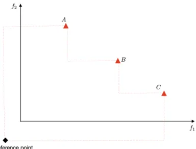
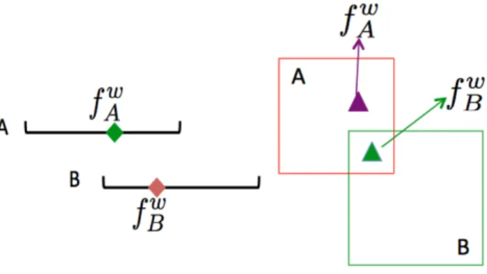
Each upper level solution is represented by an envelope. The non-dominance relationship can be extended to the upper level solutions. We use two figures to explain this concept. Solution 1 and 2 are represented by blue squares and red triangles, respectively. Considering the upper level maximises two objectivesf1 and
f2, solution 1 is dominated by solution 2 from Figure 3.5. Another example is shown
in Figure 3.6, the dashed line indicates the overall Pareto front in the upper level. Both solutions 1 and 2 have contribution to the overall Pareto front, and these two solutions are defined as non-dominated with each other.
In our envelope-based algorithm, for a number of solutions that have the same rank, the marginal hypervolume of an upper level solution is used to evaluate how important it is. For a set of non-dominated solutions, the hypervolume is represented by the area dominated by all these solutions. A solution’s marginal hypervolume is defined as the area dominated by this solution excluding the other non-dominated solutions (Branke et al. 2008). As explained above, for an upper
Figure 3.5: The comparison of two upper level solutions, and the solution repre-sented by square is dominated by the solution reprerepre-sented by triangle
Figure 3.7: Hypervolume of a Pareto front for a two objectives maximisation prob-lem
level solution, its marginal hypervolume is defined as the amount of the hypervolume would reduce if it is removed. For a Pareto front that maximises two objectives, solutions A-C are the non-dominate solutions. The hypervolume is shown as the area bounded by the reference point and non-dominated solutions in Figure 3.7. The reference point is user-defined, in our case, the reference point setting is described as follow. Assume we have a two objectives maximisation problem, find the minimum objective value for each objective. Extend each minimum objective value slightly to its minimisation direction. The intersection point is set as the reference point to calculate hypervolume.
Now we explain the marginal hypervolume using Figure 3.8. Solutions 1 and 2 are non-dominated with each other and have the same rank. The Pareto front is formed by the two solutions. The total hypervolume is shown as the area between the reference point and the six points. If solution 1 is removed, then the hypervolume would reduce the amount of the blue shaded area. This amount is the marginal hypervolume of solution 1. Solutions with greater marginal hypervolume are likely to have more contributions to the overall Pareto front. They are considered to be more important with more chance to be preferred in the upper level selection. In the envelope-based algorithm framework, given an upper level solution, the lower level algorithm obtains a Pareto front that is defined as an envelope. It is clear that each upper level solution maps to an envelope in the objective space. Non-dominate sort the upper level solutions will be the same as non-dominate sort
Figure 3.8: Marginal hypervolume of upper level solutions
a set of envelopes. We describe the non-dominated sorting in the upper level pop-ulation. Firstly, combine all the envelopes and find the overall Pareto front, for those envelopes who have more than one point contributing to the overall Pareto front, they are non-dominated with each other. Those corresponding upper level solutions are the first non-dominated front, each upper level solution in this first non-dominated front is assigned a rank 0. Then find the next non-dominated front, all the upper level solutions in the first non-dominated front will be discounted. Assign a rank 1 to each upper level solution in the second non-dominated front. Repeat this procedure until each individual in the upper level solution is assigned a rank. In order to compare the non-dominated upper level solutions, we introduce marginal hypervolume measure the quality. An upper level solution is considered to better if it has a greater marginal hypervolume.
As in the point-based algorithm, a lower level run that does not identify the true (worst case) trade-o↵might appear attractive in the upper level. So all surviv-ing individuals are re-evaluated in every generation. The new envelope (obtained by re-evaluation) is combined with the old one (before re-evaluation), and the best (f(x0), ) combinations are kept based on a non-dominated sorting and crowding distance calculations.
3.3
Empirical evaluation
In this section, we empirically compare the two proposed algorithms using a simple test function for which we can easily derive the optimum, and a test function taken from the literature. The two algorithms are further compared using a 2-dimensional test function for which its true Pareto front between the worst-case quality and robustness is known.
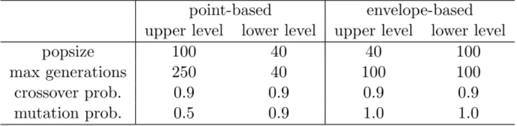
3.3.1 Parameter settings
We identified suitable parameter settings for each algorithm by some preliminary test runs. The number of solutions in the Pareto front approximation of the point-based algorithm corresponds to the number of individuals in the upper-level MOEA, whereas for the envelope-based MOEA, each individual in the upper level may con-tribute an entire envelope to the Pareto front approximation. Thus, clearly, the upper level population size of the point-based MOEA needs to be larger than for the envelope-based MOEA. On the other hand, the lower level population size needs to be larger for the envelope-based MOEA, as it needs to generate an entire enve-lope, rather than only search for a worst case. After some testing, we considered the parameter settings reported in Table 3.1 to be suitable. Table 3.2 displays the par