Determinants of the receipts from shipping services: the case of Greece

YELLOW BLACK MAGENTA CYAN

SEPTEMBER

2010

ISSN: 1105 - 9729

SEPTEMBER

2010

B

BAANNKK OOFF GGRREEEECCEE

21, E. Venizelos Avenue 102 50 Athens

www.bankofgreece.gr

Economic Research Department - Secretariat Tel. ++30 210 320 2393

Fax ++30 210 323 3025 Printed in Athens, Greece

at the Bank of Greece Printing Works ISSN 1105 - 9729

C O N T E N T S

Theodoros Mitrakos Panos Tsakloglou

Ioannis Cholezas 7

DETERMINANTS OF THE RECEIPTS FROM SHIPPING SERVICES: THE CASE OF GREECE

Zacharias Bragoudakis

Stelios Panagiotou 41

THE IMPACT OF NOMINAL AND REAL UNCERTAINTY ON MACROECONOMIC AGGRE-GATES IN GREECE

Heather D. Gibson

Hiona Balfousia 57

WORKING PAPERS

(March 2010 – June 2010) 73

ARTICLES PUBLISHED IN PREVIOUS ISSUES

1 INTRODUCTION

In a previous study the authors established that, despite the increase in graduate unem-ployment over the last two decades and the high unemployment rates of tertiary educa-tion graduates during the first years after completion of their studies, graduation from a tertiary education institution provides a cer-tain security against unemployment in the long run, at least in comparison to the lower levels of the education system (Mitrakos, Tsakloglou and Cholezas, 2010). However, lower unemployment rates alone cannot be taken as conclusive evidence of whether ter-tiary education is a good investment. To answer such a question, one also needs to know the rate of return to each level of edu-cation, or otherwise the wages that can be expected after graduation from a specific branch of the education system.

The literature on returns to education in our country (briefly reviewed below) is quite exten-sive. However, mainly on account of insuffi-cient appropriate statistical information, so far no attempt has been made in the available empirical studies to estimate (private) returns to education for small homogeneous groups of graduates by field of study. The present study aims to fill this gap by using the wage data included in the Labour Force Surveys (LFSs) conducted in Greece in the period from the first quarter of 2004 to the third quarter of 2007 (2004 I – 2007 III).

The following section briefly reviews the find-ings of the available earlier empirical studies

on returns to education in Greece. The third section describes the LFSs used in the empir-ical analysis, while the fourth section presents its major results. The last section summarises the study’s conclusions, while detailed infor-mation is included in the Appendices.

2 LITERATURE REVIEW

The issue of wage differentials between vari-ous education levels in Greece has been exam-ined mainly in the context of exploring returns to education (primarily “private” returns). In comparison to other countries, studies calcu-lating returns to education in Greece are lim-ited in number, as well as partly in depth, owing mainly to limitations of the available sta-tistical information. The question of returns to education in Greece was first explored by Leibenstein (1967). Since then, relevant research work has been prolific.1

Published studies cover the time period from 1957 until today and draw on many different databases. Relying mostly on data collected by the Hellenic Statistical Authority (ELSTAT) – from Household Budget Surveys, European Community Household Panel, European

** The views expressed in this study do not necessarily reflect those of the Bank of Greece. The authors would like to thank H. Gib-son, N. Kastis, I. Kalogirou, E. Kikilias, D. Nikolitsas, E. Papa-petrou, T. Politis and G. Psacharopoulos for their useful com-ments. The present paper was supported by the cultural project “Protovoulia” (Educational and Development Initiative), as an earlier version formed part of a broader action of Protovoulia (“Education and Development: Connecting Education and Employment”).

11 For a detailed review of the literature on private returns to edu-cation in Greece, see Cholezas and Tsakloglou (1999) and Cholezas (2005).

Theodoros Mitrakos

Economic Research Department

Panos Tsakloglou

Athens University of Economics and Business

Ioannis Cholezas

Union Statistics on Income and Living Con-ditions, etc.– they also use wage data collected by public and private enterprises, or even pri-vate researchers. Thus, it is not always easy to assess the quality and suitability of the infor-mation included in each database. All datasets used in the existing studies are cross-sectional.

As regards methodology, most earlier studies apply the Ordinary Least Squares (OLS) method to estimate Mincer’s (1974) ‘classical’ semi-logarithmic human capital equation and calculate the effect of education on earnings. In general, the “education” variable is expressed either in years or in education lev-els with the use of dummy variables, while additional explanatory variables (such as potential experience and its square, or the age and education level of the father) are often used to improve the model’s explanatory power. Heckman’s two-step method for cor-recting the sample bias or selection error is used by Kanellopoulos (1997) to determine the returns for individuals working in the public sector, as well as by Kanellopoulos and Mavro-maras (2002) who attempt to explain wage dif-ferentials between men and women. In addi-tion, Papapetrou (2004) uses the quantiles regression method, which allows an estimation of the independent variables’ effect on the dependent variable along the distribution of the latter. Finally, Leibenstein (1967), Psacharopoulos (1982), Magoula and Psacharopoulos (1999), and Kanellopoulos, Mavromaras and Mitrakos (2003) calculate social returns to education using cost-benefit techniques.

Almost all results of the available empirical studies are consistent with human capital the-ory, as they confirm a positive effect of edu-cation and potential experience on earnings. Returns to education levels increase with the years of schooling, and all additional variables have the expected signs. Of course such returns may in fact differ considerably among individuals, depending on, e.g., their mental abilities, or the particular institution they

studied at (in terms of its quality and repu-tation in the labour market), but these hypotheses cannot be tested using the avail-able statistical information. A further point of concern is that the widespread use of poten-tial (rather than actual) work experience as an explanatory variable may lead to a possi-bly overestimated contribution of experience, since it takes no account of periods of unem-ployment, or non-participation in the labour force due to pregnancy or other reasons, or transition between jobs, etc. Moreover, given that many studies use additional independent variables, returns to education are no longer comparable when these variables affect the estimated contribution of education to earn-ings. On the other hand, these variables enhance the model’s explanatory power and enable an exploration of the factors that affect earnings, often also revealing overes-timated returns to education.2 _Finally,

another important consideration relates to sample selection error. For instance, as regards women, only employed ones are included in the sample. However, if not cho-sen at random, i.e. if these are, e.g., primarily women with more years of schooling, or unmarried, then the sample is biased (not representative of all women) and, as a result of this selection error, estimates need to be corrected using appropriate econometric techniques.

A comparative analysis of the results of the available studies in light of the above con-siderations shows that, overall, returns to edu-cation in Greece follow a downward path until the late 1980s and increase in the course of the 1990s. Thus, the return to one additional year of schooling starts from 7.8% in 1964 (Kanellopoulos, 1985), falls to 5.8% in 1977 (Patrinos, 1992) and to 2.5% in 1985 (average for men and women, Patrinos and Lam-bropoulos, 1993), before rising again to 7.6% in 1994 (Magoula and Psacharopoulos, 1999) and then to even higher levels in 1999

22 Hence, the use of additional variables must be examined on a case-by-case basis, considering all positive and negative corollaries.

(Cholezas, 2005).3_{This ‘recovery’ of returns}

to education in the 1990s is attributed to the observed steady growth path of the Greek economy and the ensuing higher demand for skilled personnel, in parallel with the aban-donment of the specific indexation policy pur-sued in the 1980s that led to the compression of earnings. In most studies, the return to each individual education level reveals an almost linear relationship to the years of schooling, with the possible exception of ter-tiary, particularly university, education. For example, in 1994, the respective returns per year are 6.7% for higher secondary (general) education, 6.3% for technical education of the same level, 6.9% for Technological Educa-tional Institutes (TEI) and 8.7% for Univer-sities (ΑΕΙ) (Magoula and Psacharopoulos, 1999), whereas, in 1999, the corresponding figures for men (women) are 9.3% (12.5%), 9.6% (7.9%), 11.1% (21.2%) and 14.5% (16.3%) (Cholezas, 2005). In comparison with other EU Member States, according to evi-dence from European Community Household Panel (ECHP) data, in the second half of the 1990s returns appear higher in South Euro-pean countries, and Greece ranks at one of the top positions (Cholezas, 2005). Opposite conclusions are drawn by other studies (Har-mon, Walker and Westergaard-Nielsen, 2001; OECD, 2010) using, however, different databases for each country.

As regards the gender differential of return to education, although women often enjoyed lower rates of return in the past, more recent data imply a reversal of the situation, as returns to education for women today markedly sur-pass those for men. Thus, in 1964, the return to one additional year of schooling stood at 6.6% (6.5%) for male (female) employees (Kanellopoulos, 1982), while the correspon-ding rates for men (women) were 7.1% (11.4%) in 1974, 5.2% (6.4%) in 1988, 6.7% (7.8%) in 1994, and 7.2% (8.9%) in 1999 (Cholezas, 2005).

The exploration of returns to education by field of employment seems to yield more

con-stant results, since returns are usually higher in the private sector (Hadjidema, 1998). This does not mean that the wages of women or pri-vate sector employees are higher than those of men or civil servants; on the contrary, their returns to education are higher mainly because the earnings of their reference group (i.e. women or private sector employees with low qualifications, accordingly) are exceptionally low (Cholezas, 2005). For example, the wages of women working in the private sector are 37% lower than those of women working in the public sector, while the wage differential between these two groups depends on the level of earnings and seems to decrease as earnings increase (Papapetrou, 2003).

The coefficient of potential experience (including tenure or not) is always positive and demonstrates the importance of past profes-sional experience in the wage-setting process. The coefficient of tenure (included only in a few studies) is positive and higher than the coefficient of experience. This implies that employers are likely to value more the expe-rience gained inside the enterprise at issue, deeming job-specific experience more impor-tant than general experience. In fact, includ-ing tenure among the independent variables lowers the return to one additional year of schooling by roughly one percentage point (Kanellopoulos, 1985). All the other variables used have the expected signs. Of particular interest is the higher return to one additional year of schooling observed for individuals whose fathers have attained a higher educa-tion level (Patrinos, 1992, 1995), as evidence of transmission of wage inequalities across generations.

The empirical literature also explores other individual questions somehow related to

33 Based on Household Budget Survey data for the period 1974-1999, Kanellopoulos, Mavromaras and Mitrakos (2003) describe a sim-ilar path of returns to education. In particular, as regards men, the authors find that returns to all education levels fell considerably between 1974 and 1988, increased significantly from 1988 to 1994, and then remained unchanged or decreased slightly between 1994 and 1999. In the case of women, the respective returns decreased considerably in the period from 1974 to 1982, before rising there-after (during 1982-1999).

returns to education. Thus, although human capital theory posits that positive returns to education result from higher productivity, fil-ter theory claims that they may be stemming from the fact that education signals to employ-ers their employees’ higher skills. In such cases education may actually represent a waste of resources, since it does not lead to increased worker productivity. The results of a number of studies on the Greek labour market (Lam-bropoulos, 1992; Magoula and Psacharopou-los, 1999; Cholezas, 2005) are not always con-sistent and tend to be influenced by the methodology adopted for the investigation of the problem.

Another point of interest related to returns to education is gender discrimination in the labour market. The existing studies show that wage differentials between men and women in Greece can largely be attributed to discrimi-nation in the labour market, since 71.5% (53.8%) of their wage differentials in 1988 (1994) cannot be explained based on differ-ences in terms of male and female human cap-ital (Kanellopoulos and Mavromaras, 2002).4

Between 1988 and 1999, the gender wage gap in the private sector slightly increases but, regardless of the methodology used, most of this differential cannot be explained by dif-ferences observed in the respective human capital stocks of men and women (Cholezas, 2005). In addition, although an important dif-ferentiation emerges between the earnings of men and women when the workers’ position along the earnings distribution (Papapetrou, 2008) and their level of education (Papa-petrou, 2007) are also taken into account, in most cases wage differentials cannot be explained by differences in the workers’ pro-ductive characteristics.

As mentioned above, so far none of the avail-able studies has estimated returns to education for individual groups of graduates within a spe-cific level of education (e.g. engineers, physi-cians, economists, etc.) and, moreover, none has used LFS data. The present study, although not primarily concerned with the estimation of

private returns to education but with an exam-ination of wage differentials between groups of workers, nevertheless attempts to fill this gap.

3 LABOUR FORCE SURVEY: BRIEF DESCRIPTION AND FIRST DESCRIPTIVE RESULTS

For the purposes of this study we used the micro-data of the quarterly LFSs conducted by the Hellenic Statistical Authority (ELSTAT) between 2004 I and 2007 III. This period was chosen because (i) the LFS data collection methodology was radically revised in 2004 and (ii) ELSTAT microdata for this period are available in the form of a rotating panel, as each member of the sample participates in the LFS for six consecutive quarters (“waves”). Since 1998 ELSTAT has been conducting the LFS on a quarterly basis (previously only in the second quarter of each year). The main pur-pose of this survey is to collect detailed data on the employment and unemployment status of household members aged 15 or over. The LFS quarterly sample of the country’s total popu-lation includes approximately 30,000 house-holds (an average sampling fraction of 0.85%), with one sixth of it rotated (replaced) every quarter, which implies at least 120,000 inter-views each year.

A final question in the LFS questionnaire – addressed only to household members working as employees – relates to their monthly earn-ings. Its exact wording is the following: “What are the total monthly earnings from your main job including extra payments paid monthly? (Data should refer to last-month payments)”. Responses can be given on the basis of nine income brackets: less than €250, €251-500, €501-750, €751-1,000, €1,001-1,250, € 1,251-1,500, €1,501-1,750, €1,751-2,000 and €2,000 or more. The present study makes use of these data, although grouped information is not so

44 According to Kanellopoulos, Mavromaras and Mitrakos (2003) this share of unexplained differential came to 87.9% in 1999 (1994: 70.7%, 1988: 46.3%).

suitable for an econometric analysis of wage differentials between members of the sample. Initially, we attempted to use the panel data of the LFS by applying appropriate econo-metric techniques in order to isolate the influ-ence of non-observable individual character-istics and calculate the “net” effect of specific education system components on the level of the employees’ hourly wages. This proved unfeasible, however, since the variation of the dependent variable (and of many independent variables to an even greater extent) per unit of observation (individual) was extremely limited over time. In other words, in the vast major-ity of cases the income bracket showed only a slight change even after six consecutive quar-ters, and all other characteristics of the employees usually remained unchanged throughout their participation in the LFS. Therefore, for the purposes of the analysis, we used cross-sectional LFS data. More specifi-cally, we used the first observation of each employee in the LFS over the period 2004 I – 2007 III. Table 1 presents the corresponding monthly wage distributions by employee edu-cation level. About 15% of the employees included in the sample did not answer the abovementioned question (replied: “Do not

know/Do not answer”) and thus were excluded from the analysis. This share does not seem to be closely related to the employ-ees’ education level, although it is slightly higher in the groups of very low and very high education levels.

For the purposes of the analysis, in the case of the “closed” income brackets we assumed that the employee’s wage was the mean of the range, while for the corresponding values of the two “open” brackets (on the top and bot-tom ends of the distribution) we used the detailed data of the Household Budget Survey conducted by ELSTAT between February 2004 and January 2005, which collects infor-mation on the level of net wages without the use of income brackets. Given that the LFS sample utilised in the analysis of the wages covered the period 2004 I – 2007 III on a quar-terly basis, the median value of each income bracket in each quarter of the LFS was adjusted for inflation, based on the Consumer Price Index data published by ELSTAT, in order for all wage data to be expressed in con-stant prices of the third quarter of 2007. Finally, to convert monthly wages into hourly earnings we used the employees’ answers to the question of how many hours per week they

Up to 250 1.5 0.7 0.6 0.4 0.5 0.2 251-500 7.4 5.6 5.3 3.1 2.5 1.3 501-750 26.8 23.7 23.8 14.9 8.6 4.5 751-1,000 30.7 28.8 26.7 29.6 18.2 12.5 1,001-1,250 12.8 16.5 15.1 23.6 25.1 19.0 1,251-1,500 4.2 7.3 7.4 10.3 16.5 15.4 1,501-1,750 1.5 2.1 2.5 2.4 5.3 9.0 1,751-2,000 0.4 0.6 1.0 0.9 2.6 6.9 2,000+ 0.2 0.4 1.5 1.1 3.3 11.9 No answer 14.6 14.3 16.3 13.6 17.3 19.3

Net monthly earnings ((€))

Education level Pre-lyceum

education Lyceum

Post-lyceum non-tertiary

education TEI ΑΕΙ Postgraduatestudies

Table 1 Distribution of employees in income brackets per education level (percentages, all

usually work in their main job. This led to the exclusion of some additional responders who stated that “they cannot define the hours they usually work, because these differ significantly from one week to the other or from one month to the other”. The resulting distributions appear in Chart 1 for six categories of employ-ees grouped according to their level of edu-cation and reveal a clear positive relationship between hourly wages and education level. The next section analyses this relationship in detail.

As regards the definition of education groups, the LFS divides the population into a large number of education categories (often rather arbitrarily, in terms of the details pro-vided). Given that this study focuses on terti-ary education graduates, we chose to group AEI and TEI graduates with as much detail as possible. In many cases, however, this was unfeasible due to the limited number of employees in the groups at issue. In the end, the criterion for keeping or merging tertiary education groups was, apart from the homo-geneity of the disciplines, the existence of a minimum number of observations (around 100 men or women) spread over a large number of years after graduation. For the lower education levels, fewer groups were formed. Moreover, it was decided to exclude from the sample a few groups with either a rather small number of observations or specific problems (graduates of special needs schools, of Open University and inter-disciplinary selection programmes, of military and law enforcement academies, of the School of Pedagogical and Technological Edu-cation (SELETE/ ASPETE) and of pedagogic academies with a two-year duration of studies). The precise equivalence between LFS educa-tion categories and those of the present study is presented in Mitrakos, Tsakloglou and Cholezas (2010) Annex II, with two exceptions due to the small number of male and female employees. The first exception involves the group of “Structural Engineering” TEI grad-uates, which has been merged here with the group of “Mechanical and Computer Engi-neering” technical school graduates (TEI). The

second exception refers to the group of IT graduates (AEI), which has been merged with the group of “Mechanical Engineering” grad-uates that also includes the relevant branch of “Computer Engineering”.

4 ECONOMETRIC RESULTS

For the purposes of this study we estimate the hourly wages of the employees included in the sample according to human capital theory. This theory – originally developed by Mincer (1958, 1974), Schultz (1961), Becker (1964), Becker and Chiswick (1966) and Ben-Porath (1967) based on the ideas of Adam Smith – attributes labour wage differentials to the dif-ferent human capital stock of the individual workers. Human capital stock determines their productivity, which, in a competitive market, determines in turn the level of their wages. Human capital consists of the knowledge, skills and abilities that individuals acquire through

formal or informal education and previous work experience (OECD, 1998), in addition to their inherent abilities. These assumptions formed the basis for the elaboration of the Mincerian wage equation (Mincer, 1974), extensively used in the literature on education economics. The empirical estimates of many such studies, as brought together by Psacharopoulos (Psacharopoulos, 1973, 1981, 1985, 1994; Psacharopoulos and Patrinos, 2004), confirm the existence of a strong posi-tive correlation between education and earn-ings, but also of considerable differences in the level of – mainly private – returns to education across various countries and time periods. Our analysis covers both broad education groups, such as those in Table 1, and narrow ones, strictly defined by the employees’ field of study. In light of the literature reviewed in the second section, we opted to estimate econo-metric equations separately for men and women (considering that even if the variables affecting their respective wage levels are the same, the effect exerted is quantitatively dif-ferent). The analysed sample consists of 29,317 men and 20,851 women, whose educational qualifications are presented in Table 2. Two further points need to be made here. First, that self-employment is widespread in Greece: 41.0% (26.1%) of all employed men (women) in the sample are self-employed. Self-employment is particularly common among those with low educational qualifications (mostly in the agricultural sector) and within specific groups of individuals with high edu-cational qualifications. Indicatively, only 25.2% of male law school graduates included in the sample are employees. Very low shares of salaried employment are also observed for male graduates of the structural engineering school (35.3%) and the medical school etc. (46.6%). The corresponding shares for the sample’s female graduates are 44.0%, 54.7% and 45.1%. With respect to these groups, a slight risk may be involved in drawing conclu-sions for all graduates of the corresponding schools based on employees alone.5_The

sec-ond point to be made is that some groups are very small, or heterogeneous, or both. This holds for “Other TEI” and “Other AEI”, and male graduates of “Languages” (as well as, to a lesser extent, for male graduates of “Social Sciences” and female graduates of “Horticul-ture and Forestry”). The results for these groups are not discussed.

The results reported in Table 2 could suggest that the sample of employees may not be ran-dom, thus calling for a two-step estimation method, i.e. an initial estimation of the prob-ability of an individual’s participation in the sample of employees, and then a subsequent estimation of the employees’ wage rates, once the relevant correction term (Inverse Mills Ratio) has been included among the explana-tory variables. However, as in all two-step esti-mation trials the relevant correction term was always statistically not significant, the results presented below were estimated using the least squares method.

Traditionally, econometric estimations of pri-vate returns to education use as dependent variable the logarithm of employees’ hourly wages, and two main explanatory variables that proxy the human capital accumulated in the employee: education and work experience. In the main part of the analysis, the dummy variables we use for education represent the highest education level and specialty attained by the employee according to the detailed information of Table 2. For work experience, we use the years since graduation and their square. The quadratic term, expected to have a negative sign in the econometric estimations, indicates that the accumulation of experience increases an individual’s earnings (albeit at a decreasing rate) and may have a negative mar-ginal effect beyond a certain point (due to the depreciation of knowledge and skills). This variable used for work experience is not ideal,

55 It should be noted that these groups of graduates feature a small number of employees and not of observations in general. Thus, although they are used as independent groups, results need to be interpreted with caution, since a large share of these graduates are not employees.

since it only approximates actual work expe-rience (overlooking any periods of

unem-ployment or withdrawal from the labour mar-ket, as well as of any work combined with

stud-Pre-lyceum education 49.6 10,090 53.6 4,218 Primary 44.4 5,988 46.6 2,645 Lower secondary 58.6 4,102 68.7 1,573 Lyceum 63.5 10,797 79.4 7,141 General lyceum 62.3 7,503 78.9 6,249 Technical lyceum 69.8 1,629 88.0 642

Post-gymnasium technical school 63.0 1,665 72.2 250

Post-lyceum non-tertiary education 69.5 2,501 83.6 2,903

IEK 69.5 2,145 84.5 2,608

Other post-lyceum education 69.6 356 76.4 295

ΤΕΙ 69.7 1,506 89.7 1,803

Structural, Mechanical & Computer Engineering 71.4 774 85.5 200 Agricultural & Food Technology 71.8 139 81.0 105

Economics & Management 68.6 416 88.4 578

Medical Sciences 65.8 146 93.0 809

Other TEI 55.2 31 89.6 111

ΑΕΙ 61.9 3,949 78.2 4,467

Structural Engineering 35.3 260 54.7 149

Mechanical Engineering & IT 69.3 486 89.1 132

Physical Sciences 77.4 368 82.1 198

Mathematics & Statistics 75.3 281 88.9 160

Medical School etc. 46.6 417 45.1 287

Horticulture & Forestry 67.3 220 90.8 97

Law School 25.2 104 44.0 235

Economics & Management 68.9 880 88.8 795

Social Sciences 72.6 64 83.2 178

Humanities 82.3 386 90.2 1,071

Languages 57.4 27 81.2 327

Physical Education & Sports 80.4 267 91.4 167

Pedagogics 96.5 144 97.3 581 Other AEI 73.4 45 81.0 90 Postgraduate studies 74.9 474 79.4 319 Postgraduate degree 73.1 286 77.6 221 Doctorate 78.2 188 85.4 98 T TOOTTAALL 5599..00 2299,,331177 7733..99 2200,,885511 Education level Men Women Percentage of

employees Number of employees Percentage ofemployees Number of employees

Table 2 Percentages of employees in the total of employed persons aged 15-64 the first

ies).6 _{This can lead to an overestimation of}

actual experience and, consequently, of its effect on wages. However, compared to the corresponding variable used in most of the works mentioned in the second part of this study (i.e., age minus the minimum years of study required for obtaining the degree minus 6), it is undoubtedly a much better proxy of the actual work experience. Given that theory sug-gests no reason to expect that the relationship between experience and earnings would be the same for all education levels and specialties, we included as independent explanatory vari-ables in the estimated equation multiplicative terms introduced between the dummy vari-ables of education levels and years since grad-uation and their square.

In addition to those that proxy the employee’s human capital stock, the analysis also uses as explanatory variables some other variables associated with the employees’ wage level. These are the region and degree of urbanisa-tion of their place of residence, the sector (public/private) in which they work, their nationality and family status, the size of the local unit and the branch of economic activity of the firm for which they work, and the year and quarter of the LFS they took part in. Most results are illustrated in charts, where the dependent variable (hourly wage) is presented as a function of the years since graduation, sep-arately for men and women. The reference group consists of single men or women (depending on the equation) who are general lyceum graduates, of Greek nationality, resi-dents of Athens, employed in a business unit of 10 or less employees, in the private (retail or wholesale) sector, and have participated in the LFS in the third quarter of 2007. The detailed results and the description of the dependent and the independent variables used in the econometric analysis can be found in Appendix I. On account of heteroskedasticity, the coefficients’ estimated standard errors were corrected using White’s method (1980). Before discussing the charts with the detailed results, it would be interesting to examine the

corresponding results for six broad education groups, namely, individuals who have com-pleted studies at pre-lyceum, lyceum (higher secondary), post-lyceum non-tertiary, TEI, AEI, and postgraduate levels. These results stem from estimations based on the variables

66 As already mentioned in the literature review, the use of potential experience as a proxy for actual work experience can lead to an overestimation of the latter’s effect on hourly wages, given that tenure is not taken into account due to the lack of necessary infor-mation in the LFS sample.

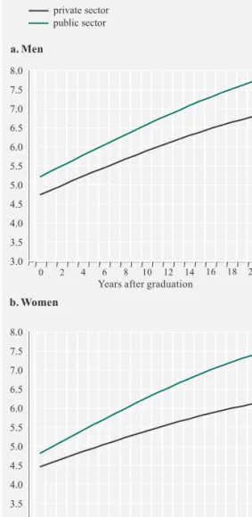
mentioned above, but this time for broader groups of graduates. They are presented in Charts 2.a and 2.b for men and women respec-tively, which depict the estimated level of employees’ hourly wages (vertical axis) as a function of the first 20 years since graduation from the highest education level completed (horizontal axis), once the effect of all other variables (family status, region, urbanisation, nationality, private or public sector, branch of economic activity, size of local business unit, quarter of the survey) has been checked. In all likelihood, twenty years after graduation is the maximum period that young people consider when deciding on the level and specialty of their studies. Similar charts are used in the rest of the study. These charts seem to fully confirm human capital theory (since the higher the education level, the higher the esti-mated level of earnings) and support our choice to introduce multiplicative terms between education level and years since grad-uation, as the slopes of the curves of the earn-ings/experience functions seem to differ con-siderably across education levels.

Charts 3.1.a to 3.7.b present similar results for homogeneous groups, usually within specific education levels, with an emphasis on the wages of tertiary education graduates. For comparison purposes, all charts also include the curve of the estimated wages of the men’s reference group (male general lyceum gradu-ates). Charts 3.1.a and 3.1.b show the estimated hourly wages of men and women with low edu-cational qualifications (primary and lower sec-ondary education graduates). Most members of these groups are of a relatively old age. The “primary education” category comprises as much persons who have not finished primary school, as primary school graduates or persons who have additionally attended a few years of gymnasium (high school). As expected, the earnings of both categories are lower than those of male lyceum graduates. What is sur-prising in Chart 3.1.b is the very small differ-ence in the wages of these two groups of employees and the fact that these wages seem to register a minimal change over the years

since graduation. In other words, the accu-mulation of work experience does not seem to substantially affect the wages of the employees belonging to these categories.

Charts 3.2.a and 3.2.b refer to lyceum (higher secondary) and post-lyceum non-tertiary graduates. Graduates of higher secondary edu-cation are grouped into three subcategories: general lyceum, technical lyceum and

post-gymnasium technical schools. The first sub-category also comprises persons who have not completed tertiary education studies; the sec-ond consists of graduates of Technical Voca-tional Lyceums (TEL), Unified Multidiscipli-nary Lyceums (EPL) and Technical Vocational Institutes (TEE); and the third comprises grad-uates of Technical Vocational Schools (TES), gymnasium foreman schools and post-gymnasium mercantile marine schools. Post-lyceum non-tertiary education graduates are grouped into two subcategories: graduates of (public or private) Institutes of Vocational Training (ΙΕΚ) and graduates of other post-lyceum education institutes. The third category comprises graduates of colleges, dance schools, tourism, (non-university) foreign lan-guages, mercantile marine officers, etc. In the case of men, the estimated wages of general lyceum graduates are slightly higher than those of technical lyceum and post-gymnasium tech-nical school graduates, although differences almost disappear after a decade. The estimated wages of graduates of other post-lyceum edu-cation institutes are clearly higher than those of IEK graduates. Indeed, the wages of the lat-ter during the first five years aflat-ter graduation do not differ from the corresponding wages of general lyceum graduates; however, the gap widens later on in favour of IEK graduates. In the case of women, the picture is slightly dif-ferent. For a number of years after graduation, the wages of general lyceum and post-gymna-sium technical school graduates are almost identical, whereas those of technical lyceum graduates are lower. In the case of women, the wages of graduates of other post-lyceum edu-cation institutes of non-tertiary eduedu-cation are higher than those of IEK graduates, but dif-ferences between the two groups are not as large as in the case of men.

Charts 3.3.a and 3.3.b show the estimated hourly earnings for graduates of TEI (or, pre-viously, KATEE, i.e. Centres of Higher Tech-nical and Vocational Training). These gradu-ates have been grouped into five subcate-gories. The first has a technical orientation (“structural engineering, mechanical and

com-puter engineering”), the second results from merging the graduates of agricultural tech-nology and food techtech-nology schools ("agri-cultural and food technology"), the next two relate respectively to graduates of “econom-ics and management” and “medical (or para-medical)” sciences, while the last one (“other TEI”) comprises graduates of schools for librarians, social workers and applied arts. As mentioned earlier, due to the heterogeneity of

the latter and the small number of observa-tions, results concerning the “other TEI” cat-egory should be interpreted with extreme cau-tion and are not discussed in detail (see also the group’s wage curve in Chart 3.3.a). For both men and women, the estimated wages of agricultural and food technology graduates are lower than those of other TEI graduates. As for the rest of the categories, structural engi-neering, mechanical and computer engineer-ing graduates seem to hold a small advantage, but differences are not significant.

Because of the classification of AEI graduates (excluding postgraduates) into a large number of subcategories, the relevant results have been grouped and are presented in three sets of charts. Charts 3.4.a and 3.4.b show estimates of the hourly wages of science graduates. More specifically, estimates are presented for the groups of “structural engineering”, “mechan-ical engineering and IT”, “natural sciences” and “mathematics and statistics” graduates. Under “structural engineering” we have included graduates from schools such as civil engineering, architecture, topography, etc. “Mechanical engineering and IT” includes graduates from schools of naval engineering, electrical engineering, chemical engineering, mineralogy, etc. Under “natural sciences” we have included graduates from schools of physics, chemistry, biology (excluding medical biology) and geology. Due to the large number of self-employed “structural engineering” graduates, it might not be possible to gener-alise the results for all graduates of the schools that belong to this group.

Contrary to the charts concerning TEI grad-uates, these charts, as well as the next two sets of charts (concerning AEI graduates), reveal significant wage differentials over male gen-eral lyceum graduates. However, differences between men and women are also large. In the case of men, after the first five years “mechan-ical engineering and IT” graduates and “nat-ural sciences” graduates seem to earn the highest wages among these four groups of AEI graduates, while the wages of “mathematics

and statistics” graduates are somewhat lower. In the case of women, the estimated hourly wages of “natural sciences” graduates start at a relatively low level and in the first ten years after graduation lag behind the wages of technical university school graduates, but thereafter seem to be the highest among the four groups in the chart. For both men and women, “mathematics and statistics” gradu-ates appear to earn the lowest wages among

the four groups in the first twenty years after graduation.

Charts 3.5.a and 3.5.b illustrate the estimated hourly wages for five groups of AEI graduates: “medical school, etc.”, “horticulture and forestry”, “law school”, “economics and man-agement” and “social sciences”. Apart from medical doctors, the group “medical school, etc.” includes graduates from dentistry, phar-maceutical and veterinary schools, while the

“social sciences” group includes graduates from schools of sociology, psychology, anthro-pology, etc. Due to the high shares of self-employed among medical school and particu-larly law school graduates, it might not be pos-sible to generalise these results for all gradu-ates of these groups.

It is worth noting how the wages of “law school” graduates evolve as a function of years since graduation. Owing probably to the

mandatory traineeship that graduates of this group have to complete, their estimated hourly wages during the first years after graduation are exceptionally low, but then rapidly increase and, after a period of 12 years for women and 20 years for men, they are the highest among the groups examined. The wages of “medical school” graduates are also high, while those of female graduates of “hor-ticulture and forestry” and of male graduates of “social sciences” range at relatively low lev-els. For men and women alike, the wages of the large group of “economics and manage-ment” graduates appear to start at satisfactory levels and evolve at a relatively fast pace (espe-cially for men).

The third group of AEI graduates consists mainly of “instructor” school graduates and the relevant results are shown in Charts 3.6.a and 3.6.b, for five groups of schools: “humanities”, “languages”, “physical education and sports”, “pedagogics” and “other AEI”. As the “other AEI” group refers to graduates from schools of fine arts, medical biology, nursing, nutrition, journalism, librarianship, home economics, etc., due to its high heterogeneity and small size the corresponding estimates are not dis-cussed. The same applies to the results for male graduates of “languages”, because the relevant estimates are derived from very few observations (a problem also observed, to a lesser extent, among male social science grad-uates). Finally, the “humanities” group includes graduates from schools of Greek lit-erature, philosophy, history, archaeology, the-ology, music, theatre, etc. It is worth noting that the estimated wages for (both male and female) graduates of “pedagogics” schools seem to rise at an increasing pace the further we move away from the year of graduation. However, given that this group includes very few graduates with extensive work experience (as studies in the corresponding schools and departments were only upgraded to AEI level roughly two decades ago), this result should be interpreted with caution. Equally noteworthy is that the estimated wages for (both male and female) graduates of “physical education” and

male graduates of “humanities” start at rela-tively low levels but rapidly pick up as the years after graduation pass.7

Finally, Charts 3.7.a and 3.7.b show the results for individuals with postgraduate studies,

sep-77 It should also be noted that, based on the experience drawn from many countries, a significant share of teachers (a group overrep-resented in the above groups of graduates), when asked about their usual working hours often state just the teaching hours, overlooking any hours of preparation, etc., and so their estimated hourly wages are often overrated.

arately for Master’s degree and doctorate hold-ers.8_{In both cases, the estimated earnings start}

at relatively high levels and increase further with time. For both men and women, the wages of doctorate holders are clearly higher. How-ever, in the case of women the gap between the two groups is relatively small and seems to remain unchanged throughout the horizontal axis (years after they completed their studies), while men’s wages differ considerably early on, but gradually converge.

Charts 4.1.a to 4.2.b present some additional econometric results for male and female AEI graduates separately. In particular, Charts 4.1.a and 4.1.b illustrate the development of the two genders’ wages over time as we move further away from graduation, for individuals working in the public and the private sector, once the impact of all other factors has been isolated. Moreover, our estimation includes among the explanatory variables multiplicative terms for the sector of employment and the years since graduation. The results are quite interesting. For both men and women, the esti-mated hourly wages are higher in the public sector. Indeed, for both genders, though more markedly for women, public and private sector wages diverge as we move further away from the year of graduation.

Charts 4.2.a and 4.2.b show the corresponding differences on the basis of the employees’ nationality. Among both men and women, the estimated hourly wages of Greek nationals and of nationals from other EU countries are prac-tically the same and considerably higher than those of the employees who are non-EU nationals. This could be the result of discrim-ination and, at the same time, a serious indi-cation of the fact that the eduindi-cational qualifi-cations these persons have most probably acquired in their home countries are not par-ticularly valued in the labour market.

The results of the econometric estimations broken down by degree of urbanisation and region of the place of residence of the employ-ees are likely to also reflect differences in the cost of living in the various areas of the coun-try (relevant charts available on request). Esti-mations for both men and women show that,

ceteris paribus, wages in the urban centres, and

particularly in the greater area of Thessaloniki, are higher than in the country’s semi-urban and rural areas. As regards the development of the estimated hourly wages of male and female AEI graduates across the country’s regions, the

88 Owing to these graduates’ higher earnings, the vertical axis in these charts covers a wider range of wages than in all other charts.

results of the estimations show certain differ-ences between the samples of men and women. However, ceteris paribus, for both genders the estimated wages earned by employees are higher in the South Aegean region and lower in the regions of Central Macedonia, the Ion-ian Islands, and East Macedonia-Thrace. Many empirical studies show that, ceteris

paribus, larger enterprises pay higher wages

than smaller ones. This phenomenon has been given many alternative interpretations. In Greece, the vast majority of enterprises are either small or very small. The LFS does not provide information on the size of the enter-prise the employees work for, but only on the size of the local unit in which they are employed. This variable helps us classify under one category all the enterprises that are not too small (local unit with more than 10 employees), although of course the other category may thus include individuals working in small units of large enterprises. At any rate, the study’s results regarding the effect of the size of the local enterprise unit on the estimated hourly wages are clear: employment in small units is associ-ated with a rather large wage disadvantage. The estimated econometric equation includes additional explanatory variables. Among the various branches of economic activity, wages differ greatly. Having isolated the impact of all other factors, “education”, “extraterritorial organisations and bodies” and “mining and quarrying” are the branches that seem to offer higher wages, while employees in the branches of “agriculture and animal breeding”, “domes-tic services” and, to a lesser extent, “retail and wholesale trade” seem to receive lower wages. Also, the wages of married persons are higher (more so of married men), something that can be attributed either to a greater effort made by them or, most likely, to the fact that family allowances are recorded together with wages. Finally, the wage levels show seasonality and, particularly, a trend over time – a fact expected since real wages increased significantly during the time period covered by the LFS waves used in the present analysis.

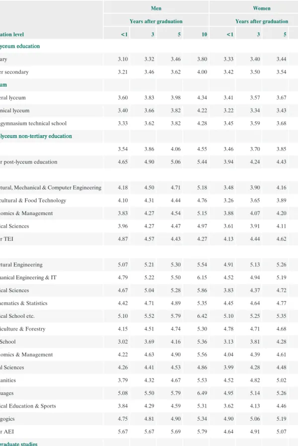
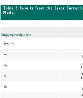
The model explains 44.3% of the dependent variable’s variation in the case of the equation for men, and 46.7% in the case of the one for women. These proportions are deemed to be quite satisfactory for the specific cross-sectional estimations of the present study. Table 3 summarises the information included in Charts 3.1.a to 3.7.b in a more comprehensible way. It presents estimated hourly wages by edu-cation level and specialty, the first year after graduation, as well as 3, 5 and 10 years after graduation, separately for men and women of

the reference group (single persons of Greek nationality that reside in Athens, work in a pri-vate sector enterprise with 10 or less employees, and have participated in the LFS in the third quarter of 2007). As regards tertiary education in particular, during the first decade after grad-uation, the graduates of “structural engineering, mechanical and computer engineering”, fol-lowed by those of “economics and manage-ment”, enjoy the highest estimated wages among TEI graduates. In some cases, the esti-mated wages of these groups are higher than the estimated wages of certain groups of AEI grad-uates. As regards AEI graduates, during the first decade after graduation, for both men and women, the highest estimated wages are observed among graduates of “medical school etc.” and of the two types of engineering schools (“structural engineering” and “mechanical engi-neering and IT”), whereas, as already men-tioned, the estimated wages of doctorate hold-ers are higher than the estimated wages of Mas-ter’s degree holders.

However, can the estimated hourly wages listed in Table 3 a priorireflect the wage that can be expected by an employed graduate of a specific education level and specialty? The answer is negative, since every stage in a per-son’s career involves the possibility of unem-ployment. In fact, as Mitrakos, Tsakloglou and Cholezas (2010) demonstrate, the estimated rates of unemployment differ significantly across education levels and specialties, and change dramatically as we move further away from the year of graduation. Therefore, in order to calculate the expected wage, the esti-mations of Table 3 should be multiplied by the probability of employment of the correspon-ding education group at the specific time inter-val from the year of graduation, as this appears in Table 4 of that earlier study (Mitrakos, Tsakloglou and Cholezas, 2010).

The resulting estimations of the present study, shown in Table 4, are evidently lower than the corresponding ones in Table 3. In several edu-cation categories, especially during the first years after graduation when the estimated

rates of unemployment are high, and more so for women than men, the estimations are much lower than those in Table 3. Nevertheless, par-ticularly after the first few years since gradu-ation, the higher the education level is, the higher the expected wage (adjusted for the probability of unemployment), with the dif-ferentials over the lowest education levels con-stantly increasing. Most of the results in Table 4 are not substantially different from those in Table 3 as to the ranking of the various spe-cialties as far as tertiary education is

con-P Prree--llyycceeuumm eedduuccaattiioonn Primary 3.10 3.32 3.46 3.80 3.33 3.40 3.44 3.53 Lower secondary 3.21 3.46 3.62 4.00 3.42 3.50 3.54 3.65 L Lyycceeuumm General lyceum 3.60 3.83 3.98 4.34 3.41 3.57 3.67 3.91 Technical lyceum 3.40 3.66 3.82 4.22 3.22 3.34 3.43 3.64 Post-gymnasium technical school 3.33 3.62 3.82 4.28 3.45 3.59 3.68 3.92

P

Poosstt--llyycceeuumm nnoonn--tteerrttiiaarryy eedduuccaattiioonn

IEK 3.54 3.86 4.06 4.55 3.46 3.70 3.85 4.22

Other post-lyceum education 4.65 4.90 5.06 5.44 3.94 4.24 4.43 4.83

Τ ΤΕΕΙΙ

Structural, Mechanical & Computer Engineering 4.18 4.50 4.71 5.18 3.48 3.90 4.16 4.75 Agricultural & Food Technology 4.10 4.31 4.44 4.76 3.26 3.65 3.89 4.39 Economics & Management 3.83 4.27 4.54 5.15 3.88 4.07 4.20 4.53 Medical Sciences 3.96 4.27 4.47 4.97 3.61 3.91 4.11 4.55

Other TEI 4.87 4.57 4.43 4.27 4.13 4.44 4.62 4.96

Α ΑΕΕΙΙ

Structural Engineering 5.07 5.21 5.30 5.54 4.91 5.13 5.26 5.59 Mechanical Engineering & IT 4.79 5.22 5.50 6.15 4.52 4.94 5.19 5.63 Physical Sciences 4.67 5.04 5.28 5.86 3.83 4.37 4.72 5.57 Mathematics & Statistics 4.42 4.71 4.89 5.35 4.45 4.64 4.77 5.14 Medical School etc. 5.10 5.52 5.79 6.42 5.10 5.25 5.35 5.58 Horticulture & Forestry 4.15 4.51 4.74 5.30 4.78 4.71 4.68 4.70

Law School 3.02 3.69 4.16 5.36 3.13 3.81 4.28 5.41

Economics & Management 4.22 4.63 4.90 5.56 4.04 4.39 4.61 5.12 Social Sciences 4.26 4.41 4.53 4.86 3.99 4.28 4.48 4.98

Humanities 3.79 4.32 4.67 5.53 4.52 4.82 5.02 5.51

Languages 5.08 5.50 5.79 6.49 4.95 5.14 5.26 5.55

Physical Education & Sports 3.84 4.29 4.59 5.31 3.62 4.13 4.46 5.24

Pedagogics 4.75 4.81 4.90 5.34 4.90 5.06 5.19 5.57 Other AEI 5.67 5.67 5.69 5.79 4.64 4.91 5.07 5.35 P Poossttggrraadduuaattee ssttuuddiieess Postgraduate degree 5.52 5.89 6.14 6.74 5.57 5.84 6.02 6.45 Doctorate 6.99 7.34 7.56 8.02 6.03 6.37 6.59 7.06 Education level Men Women

Years after graduation Years after graduation

<1 3 5 10 <1 3 5 10

Table 3 Estimated hourly wages 0, 3, 5 and 10 years after graduation

P Prree--llyycceeuumm eedduuccaattiioonn Primary 2.80 3.03 3.18 3.54 3.00 3.01 3.01 3.03 Lower secondary 3.05 3.29 3.45 3.83 3.13 3.18 3.20 3.29 L Lyycceeuumm General lyceum 3.36 3.62 3.78 4.18 2.99 3.16 3.27 3.53 Technical lyceum 3.15 3.45 3.63 4.07 2.60 2.76 2.87 3.14 Post-gymnasium technical school 3.14 3.44 3.65 4.13 2.95 3.09 3.19 3.45

P

Poosstt--llyycceeuumm nnoonn--tteerrttiiaarryy eedduuccaattiioonn

IEK 3.20 3.58 3.82 4.38 2.75 3.04 3.22 3.66

Other post-lyceum education 4.37 4.63 4.79 5.18 3.39 3.69 3.88 4.28

Τ ΤΕΕΙΙ

Structural, Mechanical & Computer Engineering 3.75 4.21 4.49 5.06 2.53 3.26 3.67 4.48 Agricultural & Food Technology 3.59 3.95 4.15 4.58 2.38 2.84 3.13 3.73 Economics & Management 3.40 3.96 4.29 5.01 3.07 3.33 3.50 3.90 Medical Sciences 3.14 3.80 4.17 4.88 2.72 3.23 3.55 4.21

Other TEI 4.30 4.26 4.22 4.18 2.90 3.59 3.96 4.59

Α ΑΕΕΙΙ

Structural Engineering 4.75 4.99 5.13 5.45 3.95 4.51 4.81 5.36 Mechanical Engineering & IT 4.51 4.98 5.29 5.98 4.00 4.59 4.93 5.48 Physical Sciences 3.91 4.51 4.87 5.67 2.29 3.17 3.75 5.06 Mathematics & Statistics 3.34 4.18 4.57 5.26 2.49 3.44 3.95 4.84 Medical School etc. 4.66 5.11 5.43 6.23 4.15 4.61 4.86 5.33 Horticulture & Forestry 3.88 4.28 4.54 5.16 3.61 3.61 3.66 3.93

Law School 2.99 3.66 4.14 5.34 2.80 3.52 4.02 5.23

Economics & Management 3.76 4.32 4.66 5.43 3.30 3.79 4.09 4.76 Social Sciences 3.80 4.08 4.26 4.68 2.71 3.39 3.79 4.60

Humanities 3.30 3.93 4.34 5.33 3.29 3.84 4.19 5.00

Languages 4.13 4.82 5.33 6.41 4.30 4.61 4.79 5.19

Physical Education & Sports 3.34 3.83 4.15 4.96 3.29 3.64 3.88 4.62

Pedagogics 4.43 4.56 4.69 5.21 3.84 4.25 4.51 5.15 Other AEI 5.22 5.26 5.30 5.46 3.93 4.35 4.58 4.99 P Poossttggrraadduuaattee ssttuuddiieess Postgraduate degree 5.03 5.53 5.85 6.55 4.60 5.16 5.48 6.13 Doctorate 6.49 7.02 7.33 7.95 4.93 5.62 6.00 6.73 Education level Men Women

Years after graduation Years after graduation

<1 3 5 10 <1 3 5 10

Table 4 Estimated hourly wages 0, 3, 5 and 10 years after graduation adjusted for

unemployment probability

cerned. Again, with respect to TEI, the grad-uates with the highest expected wages are those of “structural engineering, mechanical and computer engineering”, followed by those of “economics and management” (and “med-ical sciences” in the case of women), while with respect to AEI, at least during the first ten years after graduation, the highest expected wages are observed among graduates of “med-ical school etc.” and of the two types of engi-neering schools (“structural engiengi-neering” and “mechanical engineering and IT”). Things are less clear at the other end of the distribution, although graduates of “social sciences” schools feature almost invariably among the groups with the lowest expected wages. However, the fact that graduates of one spe-cialty of a specific education level may enjoy higher wages than those of another specialty of the same level does not necessarily imply that returns to education are higher for the former, as the years of study needed for the two spe-cialties might differ. The data on which the estimations appearing in Tables 3 and 4 rely allow for a calculation of the internal rate of return to the completion of studies for each education level and specialty, adjusted (or not) for unemployment effects. This has never been attempted so far in the available Greek liter-ature. Estimates of private returns to educa-tion for tertiary educaeduca-tion graduates based on the information used in Tables 3 and 4 are pre-sented in Table 5. Of course, as some of the groups of the sample at issue are relatively small, not adequately represented throughout the entire range of years since graduation, or showing high percentages of self-employment, the corresponding results should be treated with caution. The methodology applied is thor-oughly described in Appendix II, including a detailed example (calculation of the annual marginal private returns to education in the years after graduation from lyceum for male and female AEI graduates of “economics and management” schools).

First of all, it should be noted that due to the use of multiplicative terms between education

levels and specialties and years since gradua-tion and their square, returns to educagradua-tion resulting from the analysis are not invariable, but change as we move further away from the year of graduation. The calculation of such returns relies on a number of assumptions. As regards TEI graduates, we assume that they come mainly from technical lyceums, so their estimated wages are compared with those of technical lyceum graduates. Given that the lat-ter are lower than the wages of general lyceum graduates, if TEI graduates actually come mainly from general lyceums, their returns are overestimated in the tables.9 _{Until recently,}

studies in TEI (or formerly KATEE) lasted three years. However, since 2001 the required duration of studies for all TEI (for certain ones already since 1999) has been changed to four years. Thus, owing to the rather limited number of TEI graduates with four years of studies in our sample, the estimates presented below rely on the assumption that TEI studies have lasted three years for all TEI graduates. Obviously, the estimated internal rates of return would be lower had we assumed a four-year duration of studies. Similarly, we assumed that studies in technical university as well as “horticulture and forestry” schools last five years. Returns for “medical school etc.” graduates were also cal-culated based on the assumption of five-year-long studies because, although medical school studies last six years, other schools of that group are completed in only five or even four years. Again here the estimated internal rates of return would have been lower had we assumed a shorter duration of studies. For all other AEI graduates, the assumption made was that their studies lasted four years. For postgraduate degree holders it was assumed that studies after lyceum lasted five years; therefore, if post-graduate studies last mainly two years and most

99 It should be recalled that the return to each education level is derived by comparing the estimated coefficient of the dummy vari-able of the given level with the corresponding estimated coefficient of the dummy variable of the immediately preceding education level (marginal return). Therefore, the assumption about the spe-cific kind of education level the individuals come from (e.g. tech-nical or general lyceum) before finishing their highest level of stud-ies (e.g. TEI) is quite significant for the calculation, since it is one of the equation’s terms.

of the graduates come from schools with five or more years of bachelor studies, then the corre-sponding returns are overestimated in the tables. Finally, it was assumed that eight years of studies after lyceum are required in order to obtain a doctorate.

Needless to say, estimates in Table 5 focus on the pecuniary private returns to education, ignoring other (non-pecuniary) benefits stu-dents may enjoy thanks to their participation in higher levels of the education system. In order to calculate the returns listed in these tables, we assume that the individuals’ work-ing life is 35 years. This is most likely

realis-tic for men, but could be somewhat exagger-ated for women, at least currently (although recent developments in retirement age limits point to this direction). In the literature, work-ing life is often estimated based on a person’s (theoretical) graduation year and (theoretical) retirement age. In the case of Greece, how-ever, this would translate into lyceum gradu-ates with up to 46 years of work experience as employees. However, our sample includes very few workers (and almost no employees) with such characteristics.

In the literature, estimates such as those listed in Table 5 are usually called “private returns

Τ ΤΕΕΙΙ

Structural, Mechanical & Computer Engineering 6.8 7.2 7.0 8.4

Agricultural & Food Technology 3.9 3.4 3.6 1.0

Economics & Management 5.4 7.5 5.5 6.9

Medical Sciences 6.1 6.4 5.8 7.8

Other TEI 3.6 8.8 3.7 9.2

Α ΑΕΕΙΙ

Structural Engineering 5.2 7.4 5.5 7.9

Mechanical Engineering & IT 7.0 5.7 7.1 6.9

Physical Sciences 7.8 8.2 7.4 7.3

Mathematics & Statistics 5.7 7.8 5.3 7.0

Medical School etc. 7.9 7.4 7.9 8.0

Horticulture & Forestry 4.0 4.7 4.2 3.9

Law School 5.5 7.0 6.2 8.1

Economics & Management 6.4 6.6 6.5 6.9

Social Sciences 4.1 6.7 3.8 6.2

Humanities 5.8 8.9 5.7 8.3

Languages 10.5 9.2 9.9 9.8

Physical Education & Sports 5.3 6.5 4.8 6.8

Pedagogics 8.7 10.0 8.9 9.9 Other AEI 8.6 6.9 7.9 7.1 P Poossttggrraadduuaattee ssttuuddiieess Postgraduate degree 9.3 10.5 9.3 11.5 Doctorate 7.8 7.4 8.0 8.0 Education level

Not adjusted for unemployment

probability Adjusted for unemployment probability

Men Women Men Women

Table 5 Estimated private returns to education

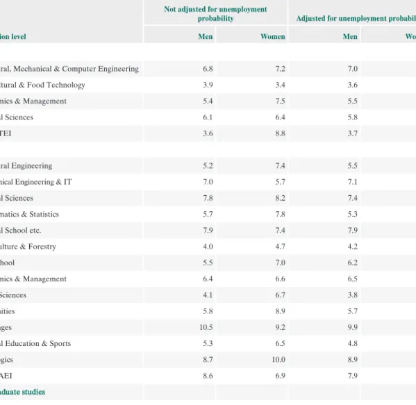
to education”. The results of Table 5 show the annual estimated returns to education, sepa-rately for men and women, by category of ter-tiary education graduates. Even though ―as shown by the results in Table 3― women’s wages are much lower than those of men, for both AEI and TEI graduates, in most cases returns to education are higher for women than for men. Of course this is mainly attrib-utable to the fact that the gap between lyceum and tertiary education graduates is, respec-tively, even greater for women than for men. Also, returns to AEI studies seem to be higher than those on TEI studies, although vast dif-ferences appear between groups of schools within the two types of tertiary education. In general, the level of returns can be considered satisfactory. The highest returns are observed for graduates of “pedagogics” (a result that, as mentioned earlier, should be treated with cau-tion), “foreign languages” (mostly women), “natural sciences” and, to a lesser extent, “medical school etc.”, while at the opposite end we find those of “horticulture and forestry” and “social sciences” (only men). The returns of Master’s degree and doctorate hold-ers are particularly high.

If we consider that investment in human cap-ital is really a form of investment, in estimat-ing its return one should also take into account the cost of the potential risks involved. Most probably, the greatest risk is that of unem-ployment, which could wipe out (at an indi-vidual level) or considerably decrease (at a collective level) expected returns. Hence, we consider that real private returns to education are those resulting from the estimations shown in Table 4 and presented in Table 5. The cal-culation of the returns in question has taken into account the probability of unemployment for a specific number of years after gradua-tion, as much for individuals in the reference group (general or technical lyceum graduates) as for graduates of every group of tertiary edu-cation.

Differences between the estimates of Table 5 are not very pronounced. The estimated

annual returns to education may increase in some cases or decrease in others, but all such changes are usually small. Among the groups of TEI graduates, the highest returns seem to correspond to “structural engineering, mechanical and computer engineering” and the lowest to “agricultural and food technol-ogy”, as regards both men and women. Among AEI graduates, returns increase in the case of the two categories of technical uni-versity graduates, “medical school etc.”, “law school” and, to a lesser extent, “economics and management”.

The ranking of schools according to the asso-ciated expected returns to education does not change significantly. Graduates of “pedagog-ics”, “foreign languages” (women), “medical school etc.”, “law school”, “physical sciences” and the two categories of technical university graduates, i.e. “structural engineering” and “mechanical engineering and IT”, show the highest returns, while the lowest returns are found in the groups of graduates of “horticul-ture and forestry” and “social sciences” (men). The returns for both Master’s degree and doc-torate holders appear to be even higher, while once again annual returns are remarkably higher for Master’s degree holders than for doctorate holders (despite the highest earnings of the latter).

5 CONCLUSIONS

The present study contains several findings regarding particular groups of tertiary educa-tion graduates. Some of these findings are con-sistent with the results of previous studies, while others appear for the first time in the lit-erature. The relationship between labour remuneration and education level is unques-tionably positive. The wages of tertiary edu-cation graduates are considerably higher than those of graduates of lower levels of the edu-cation system at a comparable point of their career (years since graduation). However, some very important differences are detected within various groups of graduates. Despite the

limitations of the analysis stemming from the nature of the data used in this study (grouped wage data, samples with a small number of observations with unsatisfactory dispersion in terms of work experience for specific groups of graduates, high and differing rates of self-employment in various groups of specialties, etc.), certain conclusions can safely be reached. University graduates of medical and engineering faculties, as well as Master’s degree and doctorate holders enjoy high hourly earnings, although this does not always entail higher internal rates of return compared with other specialties.

The fact that tertiary education graduates obtain higher wages does not necessarily imply that these individuals have become more pro-ductive because of their studies. It could sim-ply mean that they are more capable of using their tertiary education qualifications as a ‘sig-nalling’ mechanism vis-à-vis employers (an aspect not examined in the present study). Moreover, the returns to education examined in the present study are private returns. High private returns are not necessarily associated with high social returns, which would be indis-pensable in order to support the view that investment in tertiary education is profitable for society; even more so since no safe pre-diction can be made as to whether high private returns will carry on in the future as such, given

that skilled and specialised labour supply in Greece is expected to increase significantly due to the observed rapid expansion of “mass” ter-tiary education attendance over the last ten years.

According to a recent study by Georganta, Kandilorou and Livada (2008), 58% of the sec-ond-year students in two specific AEI (Athens University of Economics and Business and University of Macedonia) reported that they had decided to pursue tertiary education stud-ies in order to later find a better-paid job more easily. The findings of Mitrakos, Tsakloglou and Cholezas (2010) show that, indeed, grad-uation from a tertiary education institution shields against unemployment, at least in the long run. The findings of the present study also verify that tertiary education studies ensure a better-paid job and, consequently, satisfactory returns in the long run, especially in the schools and levels that seem to be most popu-lar among applicants. In conclusion, according to the results of the analysis, Greek young peo-ple seem to be making totally rational choices as regards their education. However, a ques-tion that remains to be answered is whether it is equally rational for the Greek state to keep expanding tertiary education, by either estab-lishing new AEI and TEI or creating new schools and departments in the existing insti-tutions.

Primary -0.1479 *** -0.0244

Lower secondary -0.1132 *** 0.0031

General lyceum Reference group

Technical lyceum -0.0564 * -0.0583

Post-gymnasium technical school -0.0785 ** 0.0105

IEK -0.0151 0.0128

Other post-lyceum education 0.2558 *** 0.1447

Structural, Mechanical & Computer Engineering (TEI) 0.1509 *** 0.0206 Agricultural & Food Technology (TEI) 0.1313 * -0.0461

Economics & Management (TEI) 0.0637 0.1292 ***

Medical Sciences (TEI) 0.0970 0.0558

Other TEI 0.3035 *** 0.1896

Structural Engineering 0.3433 *** 0.3644 ***

Mechanical Engineering & IT 0.2865 *** 0.2798 ***

Physical Sciences 0.2616 *** 0.1163

Mathematics & Statistics 0.2064 0.2650

Medical School etc. 0.3479 *** 0.4009 ***

Horticulture & Forestry 0.1426 * 0.3369 ***

Law School -0.1755 -0.0852

Economics & Management 0.1599 *** 0.1690 ***

Social Sciences 0.1680 0.1571 **

Humanities 0.0508 0.2819 ***

Languages 0.3442 0.3719 ***

Physical Education & Sports 0.0663 0.0578

Pedagogics 0.2768 0.3613 *** Other AEI 0.4547 * 0.3065 *** Postgraduate degree 0.4283 *** 0.4895 *** Doctorate 0.6638 *** 0.5691 *** Independent variables Coefficient Men Women

Estimation coefficients of the hourly wages logarithm

D

Deeppeennddeenntt vvaarriiaabbllee:: logarithm of hourly wages at constant prices

*** Statistically significant at the 1% level. ** Statistically significant at the 5% level. * Statistically significant at the 10% level.