Data Analytics and Wide-Area Visualization Associated with Power Systems Using Phasor Measurements

(1)

DATA ANALYTICS AND WIDE-AREA VISUALIZATION ASSOCIATED

WITH POWER SYSTEMS USING PHASOR MEASUREMENTS

A Dissertation by

IKPONMWOSA IDEHEN

Submitted to the Office of Graduate and Professional Studies of Texas A&M University

in partial fulfillment of the requirements for the degree of DOCTOR OF PHILOSOPHY

Chair of Committee, Thomas J. Overbye Committee Members, Le Xie

Timothy A. Davis Nicholas Duffield Head of Department, Miroslav M. Begovic

May 2019

Major Subject: Electrical Engineering

(2)

ii

ABSTRACT

As power system research becomes more data-driven, this study presents a framework for the analysis and visualization of phasor measurement unit (PMU) data obtained from large, interconnected systems. The proposed framework has been implemented in three steps: (a) large-scale, synthetic PMU data generation: conducted to generate research-based measurements with the inclusion of features associated with industry-grade PMU data; (b) error and event detection: conducted to assess risk levels and data accuracy of phasor measurements, and furthermore search for system events or disturbances; (c) oscillation mode visualization: conducted to present wide-area, modal information associated with large-scale power grids.

To address the challenges due to real data confidentiality, the creation of realistic, synthetic PMU measurements is proposed for research use. First, data error propagation models are generated after a study of some of the issues associated with the unique time-synchronization feature of PMUs. An analysis of some of the features of real PMU data is performed to extract some of the statistics associated with data errors. Afterwards, an approach which leverages on existing, large-scale, synthetic networks to model the constantly-changing dynamics often observed in real measurements is used to generate an initial synthetic dataset. Further inclusion of PMU-related data anomalies ensures the production of realistic, synthetic measurements fit for research purposes.

An application of different techniques based on a moving-window approach is suggested for use in the detection of events in real and synthetic PMU measurements. These fast methods rely on smaller time-windows to assess fewer measurement samples for events, classify disturbances into global or local events, and detect unreliable measurement sources. For

(3)

large-iii

scale power grids with complex dynamics, a distributed error analysis is proposed for the isolation of local dynamics prior any reliability assessment of PMU-obtained measurements.

Finally, fundamental system dynamics which are inherent in complex, interconnected power systems are made apparent through a wide-area visualization of large-scale, electric grid oscillation modes. The approach ensures a holistic interpretation of modal information given that large amounts of modal data are often generated in these complex systems irrespective of the technique that is used.

(4)

iv

DEDICATION

To God and Family

(5)

v

ACKNOWLEDGEMENTS

The journey to attaining a doctoral degree in Electrical Engineering made me realize how much I have been blessed, and how I would not have successfully completed it without people.

Firstly, I would like to appreciate my advisor and committee chair, Prof. Tom Overbye for his support. I owe my knowledge of power systems to him, as without his invaluable directions and input, I would not have reached my professional goal. It is a lifetime honor knowing he was my advisor.

My gratitude goes to my doctoral committee whose insights and contributions have been very helpful. In spite of their different time constraints, their availability in my different PhD examinations is greatly appreciated. I am also grateful for the knowledge I acquired in the classes which they taught.

I would like to acknowledge the support of my friends, colleagues and staff in the research group, both past and present in the University of Illinois at Urbana-Champaign (UIUC) and Texas A & M University (TAMU). Their support and constructive criticisms were invaluable. My appreciation goes to the UIUC staff of Robin Smith, Joyce Mast and Prosper Panumpabi. In TAMU, my appreciation goes to Komal, Won, Adam, Bin, Tamara, Ceci, Ogbonnaya, Zeyu, Wei, Alex and the entire research group. I remember a fellow colleague, Ti, who unfortunately passed away, and am glad to have known and worked with him. I am grateful to Prof. Jose Silva-Martinez, Melissa Sheldon and Katie Bryan who were a great blessing in helping me transition to Texas A&M University when I had recently just transferred to the department.

This acknowledgement is incomplete without the mention of my family and friends. The parental love, discipline and sacrifice provided to me in my early years has made possible my journey through this life. I am eternally grateful to my late, loving mom, who passed away many

(6)

vi

years ago. I am forever grateful to my hard-working dad who toiled, sacrificed all his comfort and supported my decision to go back to graduate school. To Vicky whose love, patience, support and prayers guided me through this journey, I cannot wait to experience the bright future God has in store for us. To my siblings, Osas, Egbe and Abebe, and brother-in-law Ndubuisi, thanks for all your prayers, thoughts and love. I also extend my appreciations to my cousin, Eseosa and Aunty Stella, who both would not allow me drop the ball at a time when I was in desperation; and Uyi, my cousin who always helped out with errands to get my documents mailed to me when I needed them. To an Illinois church family (Kings Assembly Church) and my friends, Olaolu Aj, Olaolu Davies, Tani Davies, Ladi, Oki, Emeka PE, Emeka Okekeocha, Olaniyi, Tola, Pat, Dinah, Uwa, Eddie and Dimeji, I say a big thank you!

(7)

vii

CONTRIBUTORS AND FUNDING SOURCES

Contributors

This work was supervised by a dissertation committee consisting of Professors Thomas Overbye, Le Xie, Nicholas Duffield of the Department of Electrical Engineering, and Professor Timothy Davis of the Department of Computer Science. The PowerWorld simulation software used for the different simulation studies and visualization efforts were provided by PowerWorld Incorporation through TAMU licensing. The synthetic power grids used in this work were developed by colleagues in the research group.

All other work conducted for the dissertation was completed by the student independently.

Funding Sources

Initial graduate study was supported by funding from the Illinois Center for a Smarter Electric Grid (ICSEG), and a 50% UIUC graduate teaching assistantship in the Fall Semester of 2016. Subsequent research funds were provided by a Power Systems Engineering Research Center (PSERC) high impact project T-57 which was titled, ‘Life-Cycle Management of Mission-Critical Systems through Certification, Commissioning, In-Service Maintenance, Remote Testing and Risk Assessment. These funds covered research studies partly at UIUC and TAMU. Support from Bonneville Power Administration (BPA) project TIP-353 is also acknowledged.

(8)

viii

LIST OF FIGURES

Page

Figure 2.1 Functional block diagram of the elements in a PMU device ...8

Figure 2.2 A 2,000-bus synthetic network ... 10

Figure 3.1 Voltage angles for GSL and signal spoof ... 22

Figure 3.2 Voltage angles for clock drift and intermittent GPS ... 22

Figure 3.3 ROCOF data for prototyped PMU voltage angles in Figure 4.1 ... 23

Figure 3.4 ROCOF data for prototyped PMU voltage angles in Figure 4.2 ... 23

Figure 3.5 Time skew error in real current angle data ... 24

Figure 3.6 Time skew error in synthetic voltage angle data... 25

Figure 3.7 IEEE documentation on data frame structure ... 26

Figure 3.8 Bit segment information in a data frame STAT field ... 27

Figure 4.1. 10-sec per unit voltage for 2 PMUs from real and simulation data ... 29

Figure 4.2. 1-min frequency measurements ... 31

Figure 4.3. 1-min voltage angle measurements ... 32

Figure 4.4. 1-min per unit voltage of 10 PMUs during generator outage ... 33

Figure 4.5. 5-sec per unit voltage magnitude ... 34

Figure 4.6. Down-sampled: 5-sample window mean and variance ... 35

Figure 4.7. Average variability and SNR of all 123 real voltage measurements ... 36

Figure 4.8. Noise in 1-min frequency measurement ... 37

Figure 4.9. Autocorrelation function for noise signal ... 38

Figure 4.10. Percentage outliers in voltage magnitude and angle ... 39

(12)

xii

Figure 4.12. Missing data samples in PMU measurements ... 42

Figure 4.13. Drop-out rates in voltage magnitude and angle measurements ... 42

Figure 4.14. Maximum drop-size in 123 PMUs ... 43

Figure 4.15. Framework for creating synthetic PMU data ... 45

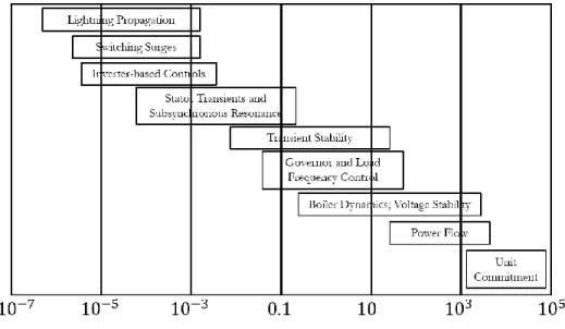
Figure 4.16. Time frames in power system operation ... 47

Figure 4.17. 24-hr load demand ... 48

Figure 4.18. Variability in simulated voltage magnitude and angle measurements ... 54

Figure 4.19. Introducing variability to simulated measurements ... 55

Figure 4.20. Per unit voltage measurements: simulation versus synthetic data ... 56

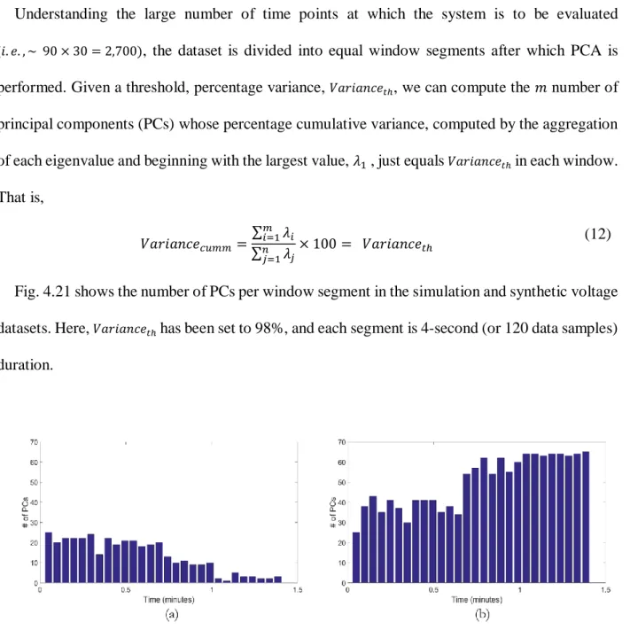
Figure 4.21. Number of principal components per window: simulation versus synthetic data ... 58

Figure 4.22. Average variability: real versus synthetic data ... 60

Figure 4.23. SNR: Real versus synthetic data ... 61

Figure 4.24. Window number of principal components: synthetic versus real data ... 61

Figure 4.25. Window variance in a VTA analysis ... 64

Figure 4.26. PCA window-window comparison on 1-min per unit voltage magnitude data ... 65

Figure 4.27. 30-min per unit voltage for all PMUs... 66

Figure 4.28. 1-sec window, e-values for 30-min duration of voltage measurements in 123 PMUs ... 67

Figure 4.29. 1-sec window, e-values for 30-min duration of voltage measurements in 123 PMUs after removal of noisy PMUs ... 68

Figure 4.30. System time-window relative disparity levels for 30-min voltage measurements ... 69

Figure 4.31. Voltage, e-values and system time-window disparities for generator trip ... 71

Figure 4.32. Voltage, e-values and system time-window disparities for generator trip, switched-in shunt and noise ... 72

Figure 4.33. 1-min, real frequency measurements around the time of generator trip ... 73

(13)

xiii

Figure 5.1 3-second voltage measurement ... 79

Figure 5.2 Wide-area search for data errors ... 80

Figure 5.3 First eight principal component vectors ... 81

Figure 5.4 Augmented voltage clustering ... 83

Figure 5.5 Pseudo-code for event data point detection and replacement ... 84

Figure 5.6 Window technique for assessing error level in data segments ... 84

Figure 5.7 Voltage magnitude measurements at all 2,000 buses and other selected buses ... 86

Figure 5.8 Event buses re-distributed to three clusters ... 87

Figure 5.9 Voltage angle measurements at all 2,000 buses, and time-skews due to time errors.. 89

Figure 5.10 Data segment errors in all 2,000 voltage magnitude measurements for error case #1 ... 92

Figure 5.11 Data segment errors in all 2,000 voltage angle measurements for error case #3 ... 93

Figure 5.12 Accumulated cost matrix for 𝑋 and 𝑌 ... 96

Figure 5.13 Prototype ROCOF patterns for internal clock delay and intermittent GPS signal .... 98

Figure 5.14 Test non-event ROCOF data 𝑇1 for case study (1) ... 99

Figure 5.15 Cut-section of accumulated cost matrix ... 100

Figure 5.16 Noise-free (𝑃1, 𝑇1) DTW distances in 𝑇1 ... 101

Figure 6.1 Periodic drop-out rates ... 106

Figure 6.2 Bit flag updates for clock drift error ... 108

Figure 6.3 Bit flag updates for intermittent GPS error ... 109

Figure 6.4 Hybrid-MDS spatial representation of noise and time errors in PMU data ... 111

Figure 6.5 Hybrid-MDS spatial representation of errors in PMU magnitude and angle data .... 112

Figure 7.1 The iterative MPA ... 114

Figure 7.2 Sensitivities of computation time and maximum cost function to number of signals ... 115

(14)

xiv

Figure 7.3 The cost functions, actual and reproduced frequency signals at 9 locations ... 117

Figure 7.4 Wide-area system cost function ... 118

Figure 7.5 (a) Wide-area cost function using voltage measurements; (b) with noise signal at bus 1017 ... 118

Figure 7.6 Phasor vector plot of mode shapes at 20 bus locations ... 120

Figure 7.7 Frequency mode shape for (a) local, and (b) inter-area modes... 121

Figure 7.8 QT clustering ... 123

Figure 7.9 Frequency mode shape for (a) inter-area mode (0.48 Hz), and (b) local mode (1.71 Hz) ... 124

Figure 7.10 Frequency coherent groups for (a) inter-area mode (0.48 Hz), and (b) local mode (1.71 Hz) ... 124

Figure 7.11 All branch oscillation energies and dissipating energy (DE) coefficients ... 127

Figure 7.12 Oscillation source and branch DE flow ... 128

Figure 7.13 Oscillation source and branch DE flow ... 129

(15)

xv

LIST OF TABLES

Page

Table 2.1. Categorization of PMU error sources ...9

Table 4.1. Noise signal attributes ... 37

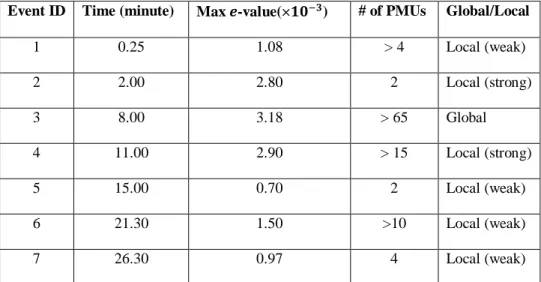
Table 4.2. Attributes of detected events ... 68

Table 5.1 LOF results for all 11 signals ... 79

Table 5.2 LOF results for all 11 signals using two sets of clustering ... 80

Table 5.3 Variance percentage of principal components - (𝑃𝐶𝑖𝑃𝐶𝑖) × 100% ... 82

Table 5.4 Summary of computed phasor magnitude LOFs (event only) ... 85

Table 5.5 Summary of computed phasor magnitude LOFs (event and noise error) ... 87

Table 5.6 Cluster formation ... 88

Table 5.7 Data errors ... 88

Table 5.8 Summary of computed phasor angle LOFs (event only) ... 89

Table 5.9 Summary of computed phasor angle LOFs (event and time errors) ... 90

Table 5.10 Summary of computed phasor angle LOFs (event, noise and time errors) ... 91

Table 5.11 LOF execution time for different system configurations ... 92

Table 6.1 Expression of binary instances ... 105

(16)

1

1 INTRODUCTION

1.1 Motivation

The 21st century, modern power grid is a large and complex interconnected system generating bulk amounts of electricity, which are transmitted and distributed to load centers where they are then harnessed for the health and prosperity of its population. For the grid to effectively carry out its function, it is essential that grid resiliency and reliability, through improved grid monitoring capabilities, be maintained at all times.

A common post-disturbance recommendation following the occurrence of major power grid outages in the United States, and other parts of the world has been that the grid, by use of sensor measurements, be closely monitored and managed [1-6]. This would ensure that operating personnel remained in control of the system in the event of any grid disturbance. For example, operators would be able to: better locate disturbance sources in need of increased damping levels when low-frequency oscillations threaten the operational state of the system, identify coherent areas in the system prior to effecting controlled islanding to minimize wide-spread outage, and better coordinate tripping actions of generators when high power capacity transmission lines are lost.

After the 2003 U.S Northeastern blackout, further recommendations for an improved wide-area situational awareness of the grid finally led to the development and deployment of high-reporting sensor devices—the phasor measurement units (PMUs) and other similar synchrophasor devices equipped to measure power system quantities at rates as high as 120 samples per second in 60 Hz operating systems [7-9]. PMUs provide time-synchronized phasor measurements,

(17)

2

otherwise known as synchrophasors, through the aid of a time reference that is provided by a global positioning system (GPS) signal. This enables the wide-area monitoring and control of a grid by making use of measurements obtained from remote locations.

As of September 2017, it was reported that over 2,500 networked PMU devices had been installed on the North American grid [10]. Consequently, large amounts of data can now be generated, and this presents several opportunities for monitoring personnel to have a higher level of visibility of the system. However, the sudden data deluge also presents the operator with a dilemma of fully uncovering and interpreting the operational state of the system. Nonetheless, following from research efforts like those in [11-17], visual displays have become welcomed tools for presenting power system data in formats that are intuitive, thus reducing the challenges faced by operators in interpreting reported grid data.

Power grids are evolving in scale, and improved methods for presenting system information have been suggested. As one of its overarching objectives, [18] emphasizes the need for intelligent data analytics and improved visualization for presenting power system data in a manner that comprehensively describes the state of the grid. The goal is to support informed and coordinated decisions taken by control center operators to ensure that the grid remains in a good operational state.

1.2 Current Technologies and Challenges

Inaccessibility to real synchrophasor or PMU data causes several data-driven power system research activities to make use of laboratory, simulation data. Several power systems simulation software, such as PowerWorld, Power System Simulator for Engineering (PSS/E), Power Systems Computer-Aided Design (PSCAD), and a host of others have been known to generate

(18)

3

experimental, research-based data for analysis. Because they do not capture the normal variations of real grids, simulation data is often devoid of the normal trending features in real PMU data. Also, they do not take into consideration the system and measurement errors that make these real data unique. The use of error-free, simulation data without the features contained in industry-grade data may result in extreme predictions which do not take into account the true variability features in PMU measurements [19].

Like most measurement devices, a failure in the operational mode of a PMU device introduces data errors in reported measurements. In addition, considering the unique mode of operation (such as time synchronization and time stamping [3, 20]), data measurements reported from this device are now exposed to a new paradigm of time-based errors. High quality of reported data can no longer be guaranteed when errors are significantly present in data measurements.

The ability to report phasor angle measurements makes the PMU a critical device in various monitoring aspects of the grid. For example, the level of grid stress is monitored by checking the phase angle differences between nodes on the system, and which could not be done through the use of conventional devices like the remote terminal units (RTUs) and supervisory control and data acquisition (SCADA) devices [3, 8] However, it is important that PMU devices be accurately synchronized to an external reference, otherwise device time errors, which causes mis-synchronization and angle measurement errors, could cause Engineers to lose sight of the true stress levels on the grid.

To aid the identification of time errors, the IEEE documentation on the standard for synchrophasor data transfer, IEEE C37.118.2 [21], has incorporated time and message quality flag bits in every data frame of the C37.118.2 data transfer protocol used by PMU devices for transmitting measured data. These flag bits provide information about the status of time

(19)

4

synchronization and data quality of data recorded by the device. The authors of [22] mention some of the different means by which a dataset can lose its attribute of logical consistency through data mislabeling, duplication, erroneous time stamps and wrong identifiers. These have the potential of rendering measurement data unintelligible, and making power engineers lose sight of the presence and source of data anomalies. A practical example of an instance of data inconsistency is the real-time issue of mislabeled C37.118 flag bits reported by [23]. Also, [22] notes the possible transformations which occur during the data archival process, such that a chain of data-handling procedures exposes PMU data to instances of possible loss or corruption. Finally, [24] reported on data inconsistencies which could arise because of possible data packing issues during data transmission from a data concentrator to a data archive.

The large amounts of PMU grid data available to control centers improves the ability to track the health of the system. As one of the critical monitoring tasks, oscillation monitoring and control plays an important role in ensuring a safe and secure operation of the grid [25-27]. Current methods used for the visualization of power system data [14, 15, 28-30] often present oscillation information on a bus node or limited area basis. However, as mentioned by [18], it is more critical for engineers to have a comprehensive picture of system states when monitoring the evolution of grid trends and dynamics. Moreover, as the grid becomes more interconnected and larger in scale, it becomes more important for data presentation methods to provide holistic perspectives of the grid to system operators.

Synthetic PMU Data

An existing challenge for studying PMU data is the sourcing of actual industry PMU data due to several confidentiality issues. When available, they are often devoid of system event signatures, such as geomagnetic disturbances (GMDs), power flow oscillations and data

(20)

5

measurement errors. These challenges often prompt the use of artificially-generated data for study and research purposes.

1.3 Organization

The major contribution of this work is the implementation of data analytic methods and visualization of large-scale grids through the use of phasor measurements. It utilizes techniques to carry out data error detection in a large-scale system, formulates methods to present wide-area PMU error information, proposes a similarity-based technique to detect time-based errors in phasor measurements, and implements a wide-area visualization platform for large-scale oscillation results. These contributions have been hinged on the generation of realistic, research-grade synthetic data due to the confidentiality issues associate with the use of real PMU measurements.

A literature review is carried out in chapter 2. It summarizes data quality issues associated with PMU measurements, data error analytic techniques and oscillation monitoring, and the contributions of this work in these areas are also highlighted. In chapter 3, different mechanisms leading to PMU data errors are discussed. The purpose is to generate error propagation models, which are used to generate synthetic data errors for use in subsequent chapters. In chapter 4, a framework for the creation of realistic, synthetic PMU data is proposed. It leverages existing synthetic networks to model power system interactions that result in the variations observed in real data. Chapter 5 discusses a distributed method for data error detection in a large-scale system, and presents a similarity-based technique for assessing time errors in PMU measurements. In chapter 6, a multidimensional scaling technique is used to present the different aspects of PMU data errors, which are then displayed on a visualization dashboard interface. Wide-area visualizations of power system oscillations in large-scale electric grids, with a focus on modal estimation quality, modal

(21)

6

interactions and oscillation source detection are presented in chapter 7. Here, the goal is to provide a wide-area assessment of the system dynamics to an observer. A summary of the achievements of this work and future directions are discussed in chapter 8.

(22)

7

2 PRELIMINARY STUDIES AND CONTRIBUTIONS

An overview of the phasor measurement unit (PMU) is presented. Data quality issues associated with measurements obtained from the device is discussed in the first section. An assessment of PMU data for errors and oscillation disturbances are discussed in subsequent sections. The chapter is concluded with a summary of synthetic networks, which are being used for research purposes. Overview of phasor measurement unit

A PMU is a time-synchronization device which can be used to measure electrical quantities, such as voltage, current, frequency or rate-of-frequency, on the power grid [7, 20, 31, 32]. One of its technological advantage lies in its ability to capture measurement samples at rates much faster than other grid sensors, such as SCADA devices. In a 60 Hz operating grid, PMUs can report measurements at 10, 12, 15, 20, 30 and 60 samples per second, while there have been instances of a report rate of 120 samples per second [24]. In comparison with SCADA devices, which sample data measurements once in 2 to 4 seconds, the large amounts of data generated by PMU devices enable a higher resolution and visibility of the grid. With the aid of an external time reference, via a timing pulse from a global positioning system (GPS) signal, PMUs are able to provide accurate, time-stamped and time-synchronized measurements of more than one microsecond accuracy. This enables wide-area, time-synchronized measurements for the purpose of estimation and analysis of power system states.

(23)

8

Figure 2.1 Functional block diagram of the elements in a PMU device

External, one pulse per second (PPS) time reference obtained through a GPS receiver is used in a phase-locked loop to create sampling clock pulses, which are used for sampling analog signals (e.g. current and voltage). The quantity phasor, which consists of a magnitude and angle component, is then computed using any of the available phasor estimation techniques.

2.1 Data Errors – A PMU Data Quality Issue

According to [22], data quality encompasses the aspects of accuracy, timeliness and availability. Any activity which reduces the high-quality level of any of the aspects can be defined to be a source of error. The synchrophasor network, comprising of PMU devices, data concentrators, communication links and the phasor applications, is exposed to a variety of errors which could affect any of the reported PMU measurement quantities- voltage (or current) phasor magnitude and angle, frequency and rate of change of frequency (ROCOF). Electrical noise, due to harmonic distortions, wiring of input signals, leakage effect caused by phasor estimation windowing function, was discussed in [20, 33-35]. Time mis-synchronization issues [36-42], caused by clock delays, intermittent reception of global positioning system (GPS) signals, loose cable wiring, spoof attacks, and which lead to phasor angle errors have also been mentioned in the literature. These error types are often attributed to the internal working mechanism of the device;

(24)

9

are manifested in the data, and thus result in low quality data reported by the device. The authors in [43-45] also show that data quality issues result from of low latency, low bandwidth, data drop-offs, wrong data alignment and limited capacities of the communication network. These errors are external, and reflect the limitations of the existing PMU network infrastructure. Finally, as observed from an application level, [46] reported on how an increased deployment of endpoint phasor applications can also reduce PMU data quality.

Several categories of PMU data error sources have been identified in the literature. According to [22], PMU data were classified into groups using three levels of attributes: attributes of single data points, dataset and data stream availability. Attributes of single data point are concerned with the accuracy of the individual, time-stamped measurements, while data set attributes relate to the accuracy and logical consistency of a group of data points or an entire set of PMU data. Data set attributes are related to the condition of the underlying communication network through which PMU data are transmitted. Based on these attribute levels, [47] divided PMU error sources into three categories, and shown in Table 2.1.

Table 2.1. Categorization of PMU error sources

Categories Error Sources

Data point Accuracy, noise, phase-error, harmonic distortion, estimation

algorithms, asynchronous local behaviors (e.g. time-skew), instrument error

Dataset Status code error, improperly configured PMUs, abnormal or loss of phasor data concentrator (PDC) configuration, frequency calculation discrepancies, mislabeling due to erroneous timestamps, CRC error, invalid timestamp

Data stream Network limitations - Data loss or drop-outs, network latency; increase in endpoint applications

(25)

10

2.2 Synthetic PMU for Power Grid Studies

A critical challenge in the use of PMU data for research purposes is the confidentiality issues associated with obtaining actual field data. Even when they are made available, they are often devoid of the desired dynamic patterns which need to be studied. These challenges prompt the development of synthetic networks, which are fictitious, but realistic, models of power grids [48-54]. They are statistically similar to real power grids since they are designed with respect to publically available data e.g. size and locations of generators, population density, etc. Thus, they do not contain any critical energy infrastructure information (CEII) and can be freely shared, used in project publications and freely provided to other researchers [55]. A 60-Hz operating, synthetic 2,000-bus network spread out over the geographic region of Texas is shown in Fig. 2.2.

Figure 2.2 A 2,000-bus synthetic network

Containing 1,250 substations, 432 generators, 3,209 transmission lines and different component dynamics set up in the system, the network is designed to simulate the operation of an actual power

(26)

11

grid. More details on this, and a 10,000-bus system used in this work are presented in Appendix A.

The unique feature set of synchrophasor measurements can be attributed to the complex operation of the grid, influence of ancillary components working alongside the phasor measurement device and a host of disturbances occurring on the system [56, 57]. While synthetic networks can be used to generate artificial data for research purposes, these measurements are often devoid of actual PMU data attributes, such as inputs from random load variations and noise. Mostly comprising of only the simulated system dynamics, these measurements are not true representations of real synchrophasor datasets, and could cause researchers to make inaccurate conclusions based on idealistic, experimental results.

The production of synthetic datasets, with similar characteristics as those obtained from a PMU, can be used to circumvent some of the mentioned challenges. This will help address some of the confidentiality issues associated with accessing real data. An ability to generate artificial measurements will also aid research studies, such as the study of grid disturbances, such as GMDs/EMP, which often rely on grid data.

2.3 Wide-Area Detection of PMU Data Errors

Large-scale systems are characterized by interconnections with varying strengths of coupling among sub-networks of nodes (buses and substations). System response to actual grid events is thus non-uniform, and gives rise to varying levels of signal correlations even for the same event.

The authors of [58] explored the low dimensionality of PMU measurements to identify the source of data errors from among a data set. A two-stage state estimation technique was employed

(27)

12

by [59] to detect bad data in PMU measurements, while in [60, 61], neural network techniques were used to train historical measurements and predict an expected maximum deviation beyond which measurements were classified as bad data or outliers. However, the need to constantly update state estimators with the most recent grid model to ensure reliable results, extensive iterative computations and long training times in neural networks oftentimes, hinder the performance and accuracy of these techniques. As systems interconnect to form larger-scale grids, and system topologies become more complex, data-driven techniques which are independent of system model information and without the burden of long computation times are required to provide more robust means of detecting bad data measurements.

2.4 Oscillation Monitoring

As large amounts of synchrophasor data become more widely available from PMU devices, an important task for Engineers is to check for disturbances in the system by carrying out online oscillation analysis on these high resolution phasor measurements. A critical activity in preserving the safe operation of the power grid, the objective of oscillation analysis, monitoring and control is to search for sources of low-frequency oscillation disturbances that may threaten the stability of the system in order to eliminate them [25, 62].

Given an observed time-varying measurement, 𝑦(𝑡), the goal of modal analysis is to obtain a re-constructed signal 𝑦̂(𝑡) that is a sum of (un)damped sinusoids, and as shown in (1).

𝑦̂(𝑡) = ∑ 𝐴𝑗𝑒𝜎𝑗𝑡cos (𝜔𝑗𝑡 + 𝜙𝑗) 𝑞

𝑗=1

(1)

The 𝑗𝑡ℎ_{mode is characterized by the modal parameters: damping factor (}_𝜎

𝑗), frequency (𝜔𝑗) and

mode shape consisting of amplitue (𝐴𝑗) and phase (𝜙𝑗). The number of modes is given by 𝑞. The

(28)

13 𝑒(𝑡) = ∑‖𝑦(𝑡𝑗) − 𝑦̂(𝑡𝑗)‖₂ 2 𝑞 𝑗=1 (2)

Different modal analysis techniques have been proposed for use in power systems to reveal the underlying low frequency signals intrinsic to power system measurements. The traditional Prony analysis computes the roots of a polynomial to determine the modal frequencies of a signal. These characteristic polynomials are associated with a discrete linear prediction model (LPM) which are used to fit the observed measurements [63, 64]. In the matrix pencil technique, a singular value decomposition is performed on a Hankel matrix, after which the eigenvalues and other modal parameters are obtained [65-67]. One of the advantages of this method is its tolerance to the presence of noise in the observed measurements. A nonlinear least squares optimization method, which encapsulates the linear variables into nonlinear variables, is used by the variable projection method (VPM) to simultaneously estimate all the modal parameters [68]. However, [69] showed that the initial modes provided by the matrix pencil method are usually sufficient. Also, a fast method of dynamic mode decomposition was proposed in [70] for off-line and on-line simultaneous processing of multiple time-series signals.

The above-mentioned modal techniques can estimate modal contents contained in power system disturbance data. However, in large-scale systems, an accurate determination of all system-wide oscillation modes, while minimizing the error function in (2) within reasonable computation times can be a challenging task.

In presenting modal information, and power systems data in general, some authors have made use of visualization tools which include contour maps, dynamic objects, animations and movies to present information about system voltage, frequency, transmission line power flows and other dynamic grid information [14, 15, 28, 71, 72]. Authors in [29] make use of phasor diagrams and

(29)

14

animation to identify coherent group formations and mode shape of a specified inter-area mode at spatially distributed system nodes respectively. Using a combination of 2-D and 3-D graphs, phasor diagram and data table, [30] reports grid modal information. Spatial and temporal variation of mode amplitudes are presented in [70].

Large-scale, interconnected systems generate huge amounts of modal data, and current techniques become inadequate in presenting wide-area system information. Here, there are tendencies for the modal decomposition process to generate several component frequency and damping values, and associated with these components are mode shape and reconstructed signal

𝑦̂(𝑡) for each of the observed measurements. In addition, large amounts of processed data are also obtained from the computation of individual transmission line power flows used for the detection of oscillation sources. As mentioned in the problem statement, there is a need for an improved method to present large-scale modal information such that observers can gain better understanding of the behaior of the system.

2.5 Contributions

2.5.1 Generation of realistic synthetic PMU measurements

Here, a proposed framework is comprised of two stages. Firstly, input data made up of annual, seasonal generation, and white-noise, load variations are fed into a power flow solver. Inclusive of other actions, such as automatic controls and disturbances, a power flow solver is used to obtain monitored states of the system. Secondly, measurements obtained from the solver are further modified. Errors and other fictitious measurements, fit enough to retain system dynamics and introduce data randomness, are included to add more realism to the synthetic measurements. This work is addressed in chapter 4.

(30)

15

2.5.2 Event detection and a distributed error analysis of PMU data measurements

An application of windowing-techniques of principal component analysis, a variation trend and modal analysis is used for system event detection in real and synthetic measurements. Fast computation from the use of small time-windows, and ability to discriminate from measurement errors makes these methods attractive. This part of the work is discussed in the last section of chapter 4.

Furthermore, a data-driven technique for analyzing PMU measurements, and applied using a distributed wide-area approach on a large-scale system is proposed. The method is supported by the density-based clustering technique, and is used to assess the level of deviation of the data segments of each phasor voltage magnitude and angle measurement relative to the other phasor measurements. This work is addressed in the second section of chapter 5.

2.5.3 Similarity-based PMU time error detection

Given the unique pattern in which time-based errors manifest in PMU measurements, a post-processing technique for the source identification of PMU time-related errors which is based on the sole use of reported phasor measurements is proposed. It leverages on defined PMU error mechanisms to generate prototype data error patterns, which are then used as training sets in the error analysis and source error identification in synthetic and actual PMU data. This work is addressed in the third section of chapter 5.

2.5.4 Presentation of error information

Given that large amounts of data are generated and transmitted to control centers, a method to present the error information obtained after carrying out data error analysis is shown. Currently, there does not exist a host of research works focused on the subject of PMU data error visualization,

(31)

16

however, the method used here leverages on the use of a multidimensional scaling to view different aspects of data errors. This work is addressed in the chapter 6.

2.5.5 Wide-area visualization of large-scale electric grid oscillation modes

The focus of this work is on the visualization of power system mode oscillations, and is addressed in chapter 7. It does not dwell on the exact methods used in identifying low frequency signal disturbances, however, the results will always be applicable regardless of the chosen method.

(32)

17

3 PMU DATA ERROR MECHANISMS

*

1

To develop the contributions discussed in chapter 2, we need to generate test data which are used in subsequent stages of this work. In this chapter, we discuss the PMU error mechanisms and time error propagation models which are used to generate the synthetic data used in this work. In the next sections, prototype and actual time errors in data measurements are presented.

3.1 PMU Error Mechanisms

The unique time-synchronization aspect of PMU operation requires a prior knowledge of the operation mechanisms associated with data errors before prototype synthetic errors can be generated. Based on the developed models, the appropriate modifications are effected on bus phasor values (magnitude or/and angle). This is in addition to other no-time based errors (e.g., noise, repeated values and dropped data frames).

3.1.1 Time Errors and Error Propagation Models

A loss of synchronism between a reference coordinated universal time (UTC) signal, obtained via the use of a global positioning system (GPS) receiver, and a PMU device internal sampling clock causes time-skew errors [36-42], and have been observed to manifest as phasor angle biases in reported measurements. However, they are observed not to affect the phasor magnitude [37]. Assuming an off-nominal, system frequency of 𝑓𝑖 Hz, the phase angle deviation ∆𝛿𝜀 due to a time

error ∆𝑡𝜀, is computed as,

∆𝛿𝜀= 360∆𝑡𝜀𝑓𝑖 (1)

* _{Part of this section is reprinted with permission from “ PMU Time Error Detection Using Second-Order} Phase Angle Derivative Measurements” by I. Idehen and T.J. Overbye , Feb. 2019 IEEE Texas Power and Energy Conference (TPEC), ©2019 IEEE, with permission from IEEE

(33)

18

where 𝑓𝑖= 𝑓𝑜+ ∆𝜀, 𝑓𝑜is the nominal frequency and ∆𝜀 is the deviation from 𝑓𝑜. The component of ∆𝛿𝜀 due to ∆𝜀 is 360∆𝑡𝜀∆𝜀. ∆𝑡𝜀 is in the order of microseconds, and in normal operating conditions,

∆𝜀 ∈ (0,0.05). Ignoring ∆𝛿∆𝜀, the updated equation becomes

∆𝛿𝜀= 360∆𝑡𝜀𝑓𝑜 (2)

A corresponding phase angle error due to an observed time difference at each reported sample, however is dependent on the source of timing error. Thus, the instantaneous phase angle error introduced in any reported sample at time, 𝑡 from the moment of error initiation is given by a generalized error propagation model,

∆𝛿𝜀(𝑡) = 360∆𝑡𝜀(𝑡)𝑓𝑜 (3)

∆𝑡𝜀(𝑡) is the instantaneous, accumulated time drift (or time-skew) at time 𝑡.

PMUs report equal time-interval samples of data measurements in cycles, such that the number of data samples reported at any cycle is known as the report rate. The accumulated time drift at any sample point is dependent on the source of error.

1. Clock drift

Here, the internal clock of a PMU is observed to gradually drift away in time due to a delay, which then causes an uneven, accumulating time-interval between samples within a report cycle. A periodic, re-synchronization attempt with a GPS pulse per second (PPS) signal only resets the synchronization status of the first data sample in the next report cycle before the clock drift begins all over again. The error propagation model for this time error behavior is given as,

∆𝑡𝜀,𝑖(𝑡) = (𝑖 − 1)∆𝑡𝜀, 𝑖 = 1,2 … 𝑛 (4)

(34)

19 2. Intermittent GPS Signal

Due to issues, such as loose wiring or incorrect placement of PMU GPS receiver, the device loses connection to the GPS reference signal. A time error, due to a delay, is observed to appear uniformly on subsequent data samples. The time error is observed to appear randomly on consecutive sets of data samples when GPS connectivity is intermittent (e.g. due to loose wiring), and an accumulating time error observed on all samples during a total GPS signal loss (e.g. due to improper placement or malfunctioning of device). The models for the intermittent and total GPS siganal loss (GSL) time error behaviors are states respectively as,

∆𝑡𝜀(𝑡) = ∆𝑡𝜀 (5)

∆𝑡𝜀(𝑡) = 𝑡∆𝑡𝜀 (6)

3. Spoofing of GPS receiver signal

Here, an attacker initially acts as an authentic source of correct external reference signal to the PMU, and then attacks the device by gradually leading its signal away from the authentic GPS signal mode. The attack model is given as,

∆𝑡𝜀(𝑡) = ∆𝑡𝜀,𝑐𝑎𝑝𝑡𝑢𝑟𝑒+ 𝑡𝑑𝑡 (7)

∆𝑡𝜀,𝑐𝑎𝑝𝑡𝑢𝑟𝑒 is a time error at the instance when an attacker completely captures the device receiver,

and𝑑𝑡 is the rate of time signal divergence induced by the attacker.

3.1.2 Non-Time Related Errors

Similar to data measurements obtained from other grid-installed sensors, PMU data are prone to the effects of unwanted noisy signals, data drops due to communication issues which affect network data streaming ability and repeated measurement values.

(35)

20

Noise in data measurements is modeled as an additive, Gaussian distributed signal, which is parameterized by a zero-mean and finite variance (σ2). The standard deviation (σ), associated with each of the measurement time points, is obtained from a Signal-Noise Ratio, (SNR, which is in decibels, dB),

𝜎 = 10−𝑆𝑁𝑅 20⁄

(8) Data drop is measured by a drop-out rate attribute, and defines the rate at which packets are lost in a data stream [22]. No data is reported at time points during which packets are lost or delayed, and [21] suggests the use of NaN (not a number) or 0x8000 (-32768)- corresponding to zero values - as filler data, which are not used in actual computation.

3.1.3 Updating Derived Measurements (Frequency and ROCOF)

Depending on the type of synthetic data error that is prototyped, a re-computation of the frequency and ROCOF signals is required. Currently, no specific estimation technique for these quantities has been defined by the IEEE reference documentation [21]. However, since the power system simulation software used for this work mimics high voltage, transmission grid operations, an approach based on [20] is used. It assumes a balanced set of three-phase input signal, and devoid of the iterative computations associated with nonlinear frequency estimation associated with unbalanced inputs.

Let 𝜔(𝑡), 𝜔𝑜, Δ𝜔 and 𝜔′ denote the instantaneous, nominal, deviation values and rate of change

of angular frequencies respectively; and 𝜙𝑜, 𝜙(𝑡) denote the values of the initial and instantaneous

phase angles respectively. It follows that:

𝜔(𝑡) = 𝜔𝑜+ ∆𝜔 + 𝑡𝜔′ (9)

𝜙(𝑡) = ∫ 𝜔(𝑡) = 𝜙𝑜+ 𝑡𝜔𝑜+ 𝑡Δ𝜔 +

1 2𝑡

(36)

21

Neglecting the nominal angular velocity which is uniform for all phase angles,

𝜙(𝑡) = 𝜙𝑜+ 𝑡Δ𝜔 +

1 2𝑡

2_𝜔′ (11)

(3) is a quadratic expression in t, and expressed as: 𝜙(𝑡) = 𝑎 + 𝑏𝑡 + 𝑐𝑡2

(12) where 𝑎, 𝑏 and 𝑐 correspond to 𝜔𝑜, ∆𝜔 and 1 2⁄ 𝜔′respectively. Solving for 𝑎, 𝑏 and 𝑐, using a

least-squares methods, the frequency deviation and ROCOF are evaluated as follows:

Δ𝑓 = 𝑏

2𝜋(𝐻𝑧), 𝑓 ′₌𝑐

𝜋(𝐻𝑧/𝑠)

(13) The actual frequency, 𝑓𝑎𝑐𝑡 is then computed as:

𝑓𝑎𝑐𝑡 = 𝑓𝑜+ Δ𝑓 (14)

Alternatively, based on the implicit definition of frequency as the rate of change of phasor angle, the derived measurements can be computed in the frequency domain as,

𝑓 = 𝑠

1 + 𝑠𝑇𝜃 (15)

𝑅𝑂𝐶𝑂𝐹 = 𝑠

1 + 𝑠𝑇𝑓 (16)

where 𝑇 ~ 0.2 second is a time-delay used to capture a window of data samples.

3.2 PMU Data Prototypes for Time Error

Figs. 3.1 and 3.2 illustrate voltage angle (VA) profiles based on the time propagation models in (4) – (7). Four different PMU time error prototypes were generated using original data from a test bus in the 2,000-bus network after a 30 second simulation. Error injection is initiated at the 5th second, and exists for 20 seconds. The report rate of the PMU is 30 samples per second.

(37)

22

Figure 3.1 Voltage angles for GSL and signal spoof. Reprinted

with permission from [73]

Figure 3.2 Voltage angles for clock drift and intermittent GPS. Reprinted

with permission from [73]

In Fig. 3.1, the VA waveforms of the GPS signal loss (GSL) event and a spoofed-GPS time signal are shown. The black horizontal line is the original, steady state VA. The blue-colored GSL event has a pulse per second (PPS) time error (∆𝑡_𝜀) of 5 µs, and the red-colored spoofed signal event has a time error divergence rate (𝑑𝑡) of 1 µs/s. For each of the events, the phase angle error ∆𝛿_𝜀(𝑡) is applied uniformly on all 30 samples in a one-second reporting period prior to the next set of reported samples.

(38)

23

Fig 3.2. illustrates VA profiles due to two different causes of PMU clock time offsets – a constant 0.5 µs time error due to a drifting internal clock, and a 1.0 µs error due to intermittent GPS clock signals received by the PMU device. The green-colored ramp for the cloc drift error is indicative of the accumulatng time error at each sample. In contrast, a uniform time error is observed for all samples in the case of intermittent GPS signal.

PMUs report ROCOF data which can also be used to monitor phasor angle changes. The derived ROCOF data for the voltage angle errors are shown in Fig. 3.3 and 3.4.

Figure 3.3 ROCOF data reprinted with permission from[73] for prototyped PMU voltage angles in Figure 4.1

Figure 3.4 ROCOF data reprinted with permission from [73] for prototyped PMU voltage angles in Figure 4.2

(39)

24

Periodic ripples observed in Fig. 3.3 for both GSL and spoofed GPS signal are attributed to the small jumps in voltage angles due to the incremental time errors. However, at the point of error removal, the accumulated voltage angle deviation results in a sudden spike in the ROCOF. We observe that the GSL event generates a significant spike (0.33 Hz/sec) which is due to the large angle deviation as compared to the case of the spoofed time signal.

In Fig. 3.4, the observed uniform ROCOF measurements for a PMU internal clock offset is consistent with the periodic VA ramp-and-reset observed in Fig. 3.2. With an intermittent GPS signal, we observe a pairwise formation of positive and negative edges of ROCOF measurements.

Real Data with Time Error

A time skew error in real current measurements obtained from a 50-Hz operating system, with a report rate of 25 samples per second, is shown in Fig. 3.5, while an artificially generated one for a 60-Hz system whose PMU reports 30 samples per second is in Fig. 3.6.

(40)

25 Synthetic Data with Time Error

Figure 3.6 Time skew error in synthetic voltage angle data

3.3 Time & Message Quality in IEEE C37.118 PMU Data

As one of the four message types in the C37.118 framework, the data frame packet holds phasor measurements of the sample being reported. In addition, it contains time and message quality information about the generated data. Fig. 3.7 shows Table 5 of the IEEE documentation [21] describing component fields in a data message.

(41)

26

Figure 3.7 IEEE documentation on data frame structure

The SYNC field provides information about time synchronization and frame identification followed by a 2-byte field of the current frame size. Each data stream is identified by an IDCODE field specifying the message source or destination. Time stamp (32-bit unsigned number), fraction of second and time quality information are provided by the Second of Century (SOC) and FRACSEC fields. A 2-byte STAT field makes use of flagged bits to provide quality status - time and measurement quality - of the reported measurement quantity. Depending on the error type being prototyped, bit modifications are carried out in accordance with the IEEE documentation. Fig. 3.8 shows the information conveyed by each of the constituent bit segments in the STAT field.

(42)

27

Figure 3.8 Bit segment information in a data frame STAT field

Detailed information about the content and bit status for all 16 bit segments are provided in pages 16 and 17 of [21]. For the purpose of this work, the focus is on bit 13, which provides synchronization status information for every reported data frame. As part of a modification step after generating synthetic PMU data, this bit is altered to reflect the data error being prototyped.

3.4 Summary

In this chapter, some of the common time propagation error models associated with PMU time-based, data errors were presented. Using these models, and showing figures of phasor angle errors, we were able to observe the unique patterns when these errors appear in measurements. In subsequent chapters, we will use these models during the creation of synthetic PMU data.

(43)

28

4 GENERATION OF POWER SYSTEMS SYNTHETIC PMU DATA

In this chapter, a process for the creation of synthetic data for research purposes is presented. Based on publically-available and pre-processed data pertaining to grid generation and load patterns, these artificial data are generated from simulations carried out on a power systems simulation software. The preferred choice of a transient stability (TS) power flow solver over a steady-state power flow analysis was to capture transient effects during selected system contingencies.

4.1 Background

The unique feature set of synchrophasor (or PMU) measurements can be attributed to the complex operation of the grid, influence of ancillary components working alongside the phasor measurement device, and effects of extraneous activities on the system [56, 57, 74]. A consequence of constantly-changing consumer loads (residential, commercial and industrial), control device actions (transformer tap changing, breaker operation, shunt capacitor switching), and several range of disturbances is the consistent variation observed in high-resolution, time-series synchrophasor measurements. In addition, low-accuracy levels of instrument transformers, improperly-connected wires and phasor estimation errors cause deviations in measurements, significant affect noise levels and introduce outlier measurements often observed in actual synchrophasor data [20, 22, 33, 34, 36, 37, 75, 76] . While synthetic networks can be used to generate artificial data for research purposes, these measurements are often devoid of actual PMU data attributes, such as inputs from random load variations and noise. Mostly comprising of only simulated system dynamics, these measurements may not be true representations of real synchrophasor datasets.

(44)

29

4.1.1 Real vs Simulated Data

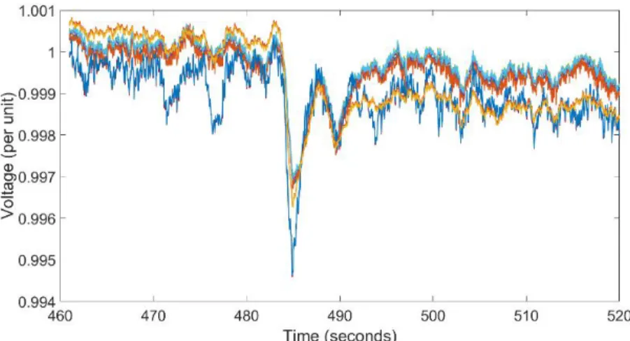
Fig. 4.1 show two sets of per unit synchrophasor voltage measurements spanning a 20-second duration, and obtained after a generator outage. The red plots in Fig. 4.1 (a) are obtained from real PMU dataset (see Appendix B), and the blue plots in Fig. 4.1 (b) are obtained from a study carried out on a power systems simulator.

(45)

30

The operating frequency for both systems is 60 Hz, and have PMU report rates of 30 samples per second. To ensure a fair comparison of both systems, the resolution on all voltage axis have been set to three decimal places. Regardless of the voltage ratings of the nodes being monitored in the real system, a trending voltage profile is observed for both PMU measurements, and is indicative of the continuous state of operation and dynamic interactions of the grid. In contrast, a predominantly, flat voltage profile is observed in the simulation data, even after an occurrence of a generator event. While there may be few measurement variations, they are mostly attributed to a pre-defined, input time step during which the grid state is evaluated. The measurements obtained from the inactive simulation system is thus a sharp contrast to those obtained from a steady, dynamics-driven, real power system. This deviation of real synchrophasor measurements from error-free simulations becomes more apparent when, in addition to system dynamics, issues such as malfunctioning PMU device components, limited network bandwidth and communication lags occur which then manifest as errors in real data.

Common features of industry-grade, PMU measurements have been identified in the literature, and they include well-damped, low-frequency system modes [25],[27, 77], disturbance events[78], measurement outliers due to system transients and noise [34, 79-81], missing data points [82], and several anomalies attributed to device errors already discussed in the prior chapter.

Fig. 4.2 shows 1-minute, real frequency data obtained from four different PMUs in the same system.

(46)

31

Figure 4.2. 1-min frequency measurements

The observations from the real PMUs are discussed thus: erroneous, constant 60-Hz frequency reported by PMU ID 106 even in the midst of grid disturbances; low frequency oscillations of 0.026-Hz and 0.069Hz observed in PMU 72, exceptional 0.2-Hz component in PMU 77, and the significant noise level in PMU 44. In contrast, simulated, error-free frequency measurements are deficient of these anomalies, and will often exhibit much lesser variations.

(47)

32

Figure 4.3. 1-min voltage angle measurements

Neglecting the slow, and true trending angle measurement samples of PMU 5, the other PMUs are a reflection of some of the several, anomalous features which can occur in industry-obtained data, and must be handled prior application usage. The observations in Fig. 4.3 are thus: PMUs 3 and 4 exhibit time-skew errors due to clock drift errors (discussed in Section 3.1); low frequency oscillations are observed in PMUs 6 and 7; and an outlier data point in PMU 6. In simulated error-free voltage angles, transitions between measurement samples are, if any, smooth, and lacking of any of the above attributes thus, causing them to differ from true industry data.

Finally, in the event of an actual contingency, the features of real measurements will often be more complex than its simulated counterpart. Fig. 4.4 is a 1-minute, voltage measurement from ten real PMUs during which there is a generator outage.

(48)

33

Figure 4.4. 1-min per unit voltage of 10 PMUs during generator outage

Voltage dip, as a result of the generator outage event is uniformly captured by all devices. Additional variations are also observed in the system, and attributed to other system dynamics which could include changing load-generation mix, local shunt-switching and the effects of operator control actions in the system. This complex, spatio-temporal relationship among PMU locations introduces features that may not be captured by simulated measurements.

4.1.2 Variability in PMU Data

Power system data measurements can be classified as non-stationary time series since the operating condition of the grid is known to evolve over time. According to [78], measurement variations of grid voltage is represented in (1).

𝜎∆𝑉𝑀

2_{= 𝜎}

∆𝑉2+ 𝜎𝜂2 (1)

𝜎∆𝑉2 and 𝜎∆𝑉𝑀

2_{are voltage signal variances before and after an introduced noise measurement}

variance, 𝜎𝜂2. While the value of 𝜎𝜂2 can be obtained directly using any of the several filtering

(49)

34

a 5-second, per-unit real voltage profile extracted from a real PMU (see appendix B for full description of real PMU dataset) with much longer duration of measurements, and a report rate of 30 samples per second.

Figure 4.5. 5-sec per unit voltage magnitude

The non-stationarity feature of this time series is observed by the continuous, seemingly-erratic state of the voltage samples. Research shows that signal-noise ratios (SNR) for most power system measurements often lie within a range of 43-47 decibels [34]. However, a computed value of 70 decibels for the first minute of this measurement proved that a high proportion of the signal was relatively noiseless. This is reflected by the three decimal-place representation before signal variations could be observed. Given a high SNR, we can assume the value of 𝜎𝜂 to be relatively

small, such that 𝜎∆𝑉_𝑀 in (1) is predominantly composed of the actual voltage variance, 𝜎∆𝑣. Further

(50)

35

The blue plot of Fig. 4.6 shows the average voltage of every non-overlapping window of five data samples, and a blue plot shows its corresponding window variance.

Figure 4.6. Down-sampled: 5-sample window mean and variance

With respect to the per-unit voltage, an average variance of 10−4_is_{observed for all windows when}

only a steady change is observed in the window average voltage, furthermore indicating the extent of total voltage variability 𝜎∆𝑣 in this clean measurement segment. Given a previous assumption of

negligible value of 𝜎𝜂, we can regard only 𝜎∆𝑣 as the only component 𝜎∆𝑉𝑀, thus providing a standard for true system voltage variability. However, in segments of the measurements where more random variations are associated with lower computed SNR values, the assumption of small 𝜎𝜂 no longer holds true.

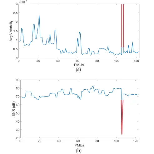
Based on the above argument, the average variability and SNR value for the first 5-second duration voltage measurement of all the real system PMUs are computed, and illustrated in Fig. 4.7 (a) and (b) respectively.

(51)

36

Figure 4.7. Average variability and SNR of all 123 real voltage measurements

The red spikes in both figures are due to the abnormal, average variability level noticed at one of the sources (with ID: 106) which was observed to have a value of 2.23×10−3_{. Neglecting this}

erroneous PMU, an average measurement variability of about 0.3 × 10−4_{(𝑖. 𝑒. , 3 × 10}−5₎_{is observed}

across the system, which is also confirmed by the almost uniform SNR values of the PMUs. Measurement Noise

The unwanted disturbance of measurement noise injects a measure of variability into synchrophasor measurements. Noise in power systems is assumed to be Gaussian, and thus modeled as a normal distribution with a zero-mean and a standard deviation. Fig. 4.8 shows the

(52)

37

first 1-minute frequency obtained from a real PMU (with ID: 44), and from which noise has been extracted.

Figure 4.8. Noise in 1-min frequency measurement

Prior to noise extraction, a moving-window, median filter [81, 83] of different orders of 90, 150 and 300 samples were tested to eliminate outlier data samples which exceeded 3-standard deviations of the median value of a moving window. The red circles in Fig. 4.8 (a) are the eliminated outliers for a filter order of 90, after which the noise signal shown in Fig. 4.8 (b) was extracted. An average mean of approximately zero, the computed SNR of 43.1 decibels is adjudged to be typical of power system measurements. Other attributes of the signal are shown in Table 4.1.

Table 4.1. Noise signal attributes

Frequency (Hz) Per unit (p.u)

Mean 4.3 × 10−4 _{7.2 × 10}−6

(53)

38

A further assessment of the signal to confirm the ‘independent and identically distributed (i.i.d)’ property of the noise signal samples can be carried out by computing an autocorrelation coefficient, 𝜌 as a function of different values of lag 𝑘 [84, 85].

𝜌𝑘=

𝐸[(𝑧𝑡− 𝜇)(𝑧𝑡+𝑘− 𝜇)] √(𝐸[(𝑧𝑡− 𝜇)2]𝐸[(𝑧𝑡+𝑘− 𝜇)2])

(2) 𝑍 is a measurement sample; 𝜇 is a constant mean over the entire range of measurements;

𝐸[(𝑧𝑡− 𝜇)(𝑧𝑡+𝑘− 𝜇)] is an auto-covariance function which measures the co-variance between any

sample that are 𝑘 distance apart; and 𝐸[(𝑧𝑡− 𝜇)2]is a self-correlation of a sample (i.e., correlation

with respect to itself). Fig. 4.9 is the generated autocorrelation function (ACF) for 𝑘 values up to 20.

Figure 4.9. Autocorrelation function for noise signal

In an ideal scenario, noise samples are independent of each other, such that at any lag, 𝑘 ≠ 0, the ACF should equal zero, and one if otherwise. Fig. 4.9 approximates this behavior with a small ACF value of less than 0.2 at 𝑘 = 1before rolling off to zero at the next lag value. Neglecting its