Abstract — This study addresses the development and Hardware-in-the-Loop (HiL) testing of an explicit nonlinear model predictive controller (eNMPC) for an anti-lock braking system (ABS) for passenger cars, actuated through an electro-hydraulic braking (EHB) unit. The control structure includes a compensation strategy to guard against performance degradation due to actuation dead times, identified through experimental tests. The eNMPC is run on an automotive rapid control prototyping unit, which shows its real-time capability with comfortable margin. A validated high-fidelity vehicle simulation model is used for the assessment of the ABS on a HiL rig equipped with the braking system hardware. The eNMPC is tested in 7 emergency braking scenarios, and its performance is benchmarked against a proportional integral derivative (PID) controller. The eNMPC results show: i) the control system robustness with respect to variations of tire-road friction condition and initial vehicle speed; and ii) a consistent and significant improvement of the stopping distance and wheel slip reference tracking, with respect to the vehicle with the PID ABS.
Index Terms — Anti-lock braking system, wheel slip control, explicit nonlinear model predictive control, hardware-in-the-loop, electro-hydraulic braking system.
I. INTRODUCTION
LECTRO-hydraulic braking (EHB) systems are becoming viable solutions for conventional, hybrid electric and fully electric vehicles, as demonstrated by the first successful implementations on series passenger cars [1-3]. In EHB systems, the brake pedal and wheel calipers are decoupled to allow pedal force feedback and, thus, pedal feeling that is independent of the operating conditions of the braking system. In addition to this driver comfort benefit, EHB units permit continuous control of each caliper pressure. This is ideal for brake blending, i.e., the seamless and variable braking torque distribution between friction brakes and electric drivetrains.
This work was supported by the European Union's Horizon 2020 Programme under Grant Agreements No. 645736 (EVE project) and No. 824254 (TELL project).
D. Tavernini (email: [email protected]), F. Vacca (email: [email protected]), M. Metzler (email: [email protected]), P. Gruber (email: [email protected]), A.E. Hartavi (email: [email protected]) and A. Sorniotti (corresponding author, email: [email protected], phone: +44 1483 689688) are with the University of Surrey, GU2 7XH Guildford, UK.
D. Savitski (email: [email protected]) is with Arrival Germany GmbH, 75179 Pforzheim, Germany.
V. Ivanov (email: [email protected]) is with the Technische Universität Ilmenau, 98693 Ilmenau, Germany.
M. Dhaens (email: [email protected]) is with Tenneco Automotive Europe BVBA, 3800 Sint-Truiden, Belgium.
Also, compared to standard braking systems with vacuum booster, EHB systems allow relatively smaller packaging and faster response times [4]. The quicker response is beneficial to the performance of active safety functions such as electronic stability control (ESC) [5].
Anti-lock braking systems (ABS) for passenger cars were developed to increase road safety by keeping the vehicle steerable and stable during intense braking events, especially on slippery road surfaces [6, 7].The first implementations used rule-based algorithms considering the estimated slip ratio and wheel deceleration. These controllers were suitable for hydraulic units capable of generating sequences of pressure increase, decrease and hold phases, but without the capability of continuous feedback control. Such algorithms were rather robust with respect to the possible operating conditions of the vehicle, but provided sub-optimal performance in terms of wheel slip tracking. Since then, improvements have been gradually implemented, at the cost of increased tuning complexity [8]. Nevertheless, today’s industrial ABS control strategies are still based on complex set of rules. EHB technology, similarly to electro-mechanical brake technology, permits more refined wheel slip controllers with continuous brake torque modulation [9]. Algorithms based on proportional integral derivative (PID) formulations [10, 11], second order sliding mode [12] as well as maximum transmissible torque estimation [13] have been proposed for ABS or traction control. [14] discusses a selection of wheel slip controllers for electric vehicles, not requiring vehicle speed detection, while [15] presents slip controllers for split- conditions.
Recent literature shows increasing interest in model-based state feedback controllers, and especially in model predictive control (MPC). In [16] an ABS based on a gain scheduled linear quadratic regulator was tested on a vehicle with electro-mechanical brake calipers. Linear MPCs are discussed in [17-19], in the context of ABS including torque blending between friction brakes and in-wheel motors. In [20] the MPC strategy is compared with a PI controller, and is assessed on an electric vehicle prototype. A linear MPC is also presented in [21], with results from a Hardware-in-the-Loop (HiL) rig including a brake-by-wire system. The study shows the deterioration of the longitudinal slip tracking performance during transitions from high to low tire-road friction levels.
[22] discusses a traction controller for an internal-combustion-engine-driven vehicle, and compares four linear MPC strategies with a hybrid explicit MPC. The performance of the hybrid strategy is comparable with that of a well-tuned PID controller. [23] presents a real-time capable implicit nonlinear model predictive controller (NMPC) for an ABS with
An explicit nonlinear model predictive ABS
controller for electro-hydraulic
braking systems
D. Tavernini, F. Vacca, M. Metzler, Graduate Student Member, IEEE, D. Savitski, Member, IEEE, V. Ivanov,
SeniorMember, IEEE, P. Gruber, A.E. Hartavi, M. Dhaens, and A. Sorniotti, Member, IEEE
torque blending, and compares the NMPC simulation results with those from a linear MPC. In addition to the better performance of the nonlinear solution, [23] reports that the computational time for the NMPC is of 3-4 ms on a desktop personal computer, whereas the linear MPC requires ~1 ms. In [24] an implicit NMPC slip control strategy is assessed in simulation, and implemented on a quad-core 2.8 GHz dSPACE unit yielding a computational time of 4-5 ms. [25] shows that the implementation time step is more influential than the selected control technology (NMPC or PID) on the performance of a traction controller for an electric vehicle with in-wheel motors. Hence, controllers with high tracking performance and low computing times are required for effective wheel slip control.
In this context, this paper presents an explicit NMPC algorithm – so called eNMPC – for ABS, and its implementation on an EHB system. eNMPC is selected as: According to many practitioners, MPC represents the future
of automotive control, since this technology: i) requires a lower number of calibration parameters than more conventional controllers, and thus reduces development times, as stated in [22, 26, 27]; ii) permits formal consideration of system constraints; and iii) allows preview control, which is of the essence in the future context of
connected and autonomous vehicles. In such
implementations, the tire-road friction estimation could be enhanced by the information from the vehicles located in front of the ego vehicle, and in general the characteristics of the road ahead are likely to be better known than in existing controllers. The eNMPC ABS of this research prepares the ground for these developments, as the tire-road friction coefficient can be included as an input parameter varying in real-time.
NMPC for ABS control offers benefits with respect to alternative control technologies, such as H∞ and sliding
mode control [10]. The main issue of H∞ control is that the
range of variation of the longitudinal tire slip stiffness is too wide to be captured by a single controller based on a linear model with a fixed longitudinal slip stiffness. Moreover, wheel slip control interventions are becoming more frequent in modern stability controllers actuating the friction brakes, which tend to operate to improve the cornering response also in sub-limit conditions, as seamlessly as possible. Hence, it is desirable to have a controller capable of a rather smooth wheel slip control action, without the typical chattering issues of sliding mode controllers.
Because of its explicit nature, the specific ABS eNMPC of this study requires only a fraction of the computing time (i.e., < 0.1 ms on a 900 MHz dSPACE automotive platform) of the implicit solutions in [23, 24], and therefore can run at much smaller time steps than an equivalent implicit NMPC. In eNMPC the explicit solution is known in advance, which
allows carrying out a systematic a-priori analysis of the control system performance, with benefits in terms of functional safety of the automotive system, with respect to implicit NMPC.
The points of novelty are:
The design and experimental implementation of a proof-of-concept eNMPC ABS based on continuous wheel slip control. The algorithm takes the experimentally measured dead time of the hydraulic components into account through a compensation strategy.
The comparison of the eNMPC ABS with a benchmark PID controller, including robustness assessment with respect to tire-road friction conditions and initial vehicle speed.
II. PLANT
A. Electro-hydraulic braking (EHB) system
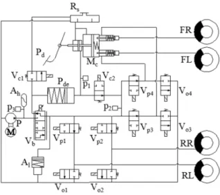
This study used the slip control boost (SCB) unit by ZF-TRW [28]. Fig. 1 shows the schematic of the hydraulic circuit of the EHB system including the four brake calipers. The notations FL FR, RL and RR indicate the front left, front right, rear left and rear right corners. The driver demand is measured in terms of brake pedal displacement (Pd) and pressure at the normally open valve Vc2, which is activated upon brake application. A brake pedal force emulator (Pde) provides force feedback to the driver. The measured signals are transmitted to the brake function control unit that calculates the caliper pressure demands. These are sent to the electro-hydraulic control unit (EHCU), which tracks them through a combination of feedback and open-loop control of the EHB valves and motor. A feedback pressure controller modulates the proportional boost valve, Vb, either to increase the brake pressure in the rail leading to the four inlet valves, Vp1 – Vp4, or to decrease it by sending the fluid back to the reservoir, Rs. The high pressure accumulator, Ah, is charged up to 180 bar by the electric pump, P, to ensure a fast system response during the pressure increase phases. In normal braking conditions, Vp1 – Vp4 remain open to permit the fluid to reach the calipers, and the four outlet valves, Vo1 – Vo4, are closed. During the operation of the ABS and stability control system, individual caliper pressure modulation is achieved through the open-loop digital control of the inlet and outlet valves. The low pressure accumulator, Al, provides the brake fluid volume displacement to prevent significant pressure oscillations.
Fig. 1. Simplified hydraulic schematic of the case study SCB unit. The wheel brake torque is proportional to caliper pressure, which generates the clamping force between pads and discs.
The torque-to-pressure coefficient, , for each corner of the -th axle (i.e., for front and for rear), is given by:
= 1
2 , , ∈ { , } (1)
where is the friction coefficient (assumed constant) between pads and disc, , is the area of the brake caliper
piston of diameter ,, i.e., , = ,, and , is the
equivalent brake disc radius. The main braking corner parameters of the case study vehicle are reported in Table I.
TABLEI.MAIN BRAKE CORNER PARAMETERS.
Symbol Description Value Unit
, Front equivalent brake disc radius 0.120 m , Rear equivalent brake disc radius 0.133 m , Front brake piston diameter 0.057 m , Rear brake piston diameter 0.040 m Brake-disc-to-pad friction coefficient 0.400 (-)
Front torque-to-pressure coefficient 0.041 bar/Nm Rear torque-to-pressure coefficient 0.075 bar/Nm B. Hardware-in-the-Loop (HiL) set-up
The HiL testing facility (Fig. 2) used for the experiments of this study consists of the following hardware components: i) The EHB system described in section II.A, with its EHCU. ii) The brake calipers and discs of the four corners of the case
study vehicle.
iii)Pressure sensors located close to the calipers to monitor the actual brake pressures.
iv)The real-time testing (RTT) platform dSPACE DS1006 (quad-core, 2.8 GHz), running a high fidelity vehicle simulation model.
The vehicle simulator is an experimentally validated (see [29], [30]) IPG CarMaker HiL model. The tire model is the Pacejka Magic Formula (ver. 5.2) [31], with varying longitudinal tire relaxation length as a function of both vertical load and longitudinal slip, as described in [32]. The experimental caliper pressure measurements are sent to the real-time vehicle simulator, which calculates the braking torque, and thus the overall vehicle dynamics, from the torque-to-pressure coefficients of the respective calipers.
Fig. 2. Hardware-in-the-Loop test rig of the Technische Universität Ilmenau.
C. EHB system characterization
Experimental tests with different caliper pressure demand ( ) profiles were carried out to determine the brake pressure response characteristics. The measurements focused on the computation of:
The dead time, Δ, i.e., the time required to achieve a 1 bar variation of the actual caliper pressure, , from when a
step is requested.
The rise time, r, i.e., the time required for to increase from 10% to 90% of its steady-state reference value during a step request.
Δ and r were assessed from 10 repeated staircase tests, consisting of 12 steps of with a 10 bar amplitude each (Fig. 3). The staircase tests simultaneously involved all four calipers, and can be considered representative of the ABS regulation condition as a non-zero pressure is present in all calipers. Figs. 4a and 4c report the average values and error bars of Δ for the front and rear calipers, as functions of the final values at each step. The magnitude of the error bar represents the standard deviation of the measured values for the 10 test repetitions. The average r values and respective error bars are shown in Figs. 4b and 4d. In addition, Fig. 5 reports the time-pressure history for a sine sweep test on the front left caliper, with an amplitude of 20 bar and a linearly increasing frequency (up to 7 Hz) of , around a value of 100 bar.
Fig. 3. Time history of a 10 bar staircase test for a front caliper.
Fig. 4. Average values and error bars of: the (a) front and (c) rear caliper pressure dead times (Δ); and the (b) front and (d) rear caliper pressure rise times (r), as a function of the final value of for 10 repetitions of the10 bar staircase test.
Fig. 5. Sine sweep test on the front left caliper: average pressure of 100 bar, reference amplitude of 20 bar, maximum frequency of 7 Hz.
The results confirm the significant nonlinearity of the system response. In particular, Δ and r tend to decrease with increasing . The average dead time, of approximately 20 ms, is long compared to the typical implementation time step of an ABS algorithm (see section I), which makes continuous wheel slip control rather difficult. Nevertheless, the EHB has very good dynamic characteristics and accurate pressure tracking capabilities relative to a conventional automotive braking system with vacuum booster.
III. EXPLICIT NONLINEAR MODEL PREDICTIVE CONTROL
A. General optimal control problem formulation
eNMPC requires the formulation of an optimization problem, where constraints on the control inputs and system states can be imposed. For a finite horizon in the time interval[ , ], a generic nonlinear optimal control problem is defined to minimize the cost function:
, , , , ( ), ,
≜ ( ( ), ( ), ( ), ( ), )
+ , ( ),
(2)
where , , and are the state, input, parameter (including system and controller parameters, considered constant for the duration of the prediction horizon) and slack variable vectors, which are internally normalized by a set of characteristic values; is time; is the stage cost; and is the terminal cost. The problem is subject to inequality constraints of the form:
≤ ( )≤ (3)
≤ ( )≤ (4)
( ( ), ( ), ( ), ( ), )≤0 . (5)
The equality constraints are the ordinary differential equations (ODEs) describing the system dynamics:
( ) = ( ( ), ( ), ( ), ) (6)
where is the vector of the system parameters. ( ) is imposed as initial condition vector.
The infinite-dimensional optimal control problem in (2)-(6) is discretized and parametrized, thus becoming a nonlinear programming (NLP) problem, which is solved through numerical methods. In this operation, known as Direct Method [33], the equality constraints (6) are represented by finite approximations. The infinite-dimensional unknown solution,
, , and the slack variables, , , are replaced by a
finite number of decision variables. The prediction horizon,
= − , is defined as = , where is the number
of prediction steps and is the discretization interval of the internal model. The input, , , is assumed piecewise constant along the horizon. is calculated through the function and is expressed through the control parametrization vector, , so that ( ) = ( , ). Similarly, the slack variable vector is parametrized through the vector , i.e., ( ) = ( , ).
The technique known as Direct Single Shooting [34–36] deals with the equality constraints. They are eliminated by substituting their discretized numerical solution (only function of the initial conditions at ) into the cost function and constraint functions. The optimal control problem is now in its multi-parametric (mp) NLP generic form:
∗ ( ), ( ) = min
, ( ( ), , ( ), ) (7)
subject to:
( ( ), , ( ), )≤0 (8)
Two additional vectors are defined: i) the problem parameter vector, ( )∈ ℝ , with = + , i.e., is the sum of the number of states, , and the number of parameters, , of the system and controller:
( ) = [ ( ), ( )] (9)
and ii) the decision variables vector, ∈ ℝ :
= [ , ] . (10)
From (9) and (10) it is possible to reformulate (7) and (8) as:
∗ ( ) = min , ( ) (11)
subject to:
, ( ) ≤0 . (12)
The minimization is performed with respect to and is parametrized with ( ).
B. Off-line solution and on-line evaluation
The mp-NLP problem is not solved directly, but through a
multi-parametric quadratic programming (mp-QP)
approximation (see [34–35]) of the mp-NLP, as suggested in [33] and implemented in [36]. The mp-NLP in (11) and (12) is linearized around a point ( , , ) by means of Taylor series expansion. The cost function is thus approximated with a quadratic function and the constraints assume a linear form.
The mp-QP formulation is used to generate local approximations of the original mp-NLP problem within the exploration space, which consists of a number of hyper-rectangles, on which single mp-QP problems are solved. Each hyper-rectangle is further partitioned into polyhedra, i.e., the critical regions for the mp-QP problem. The resulting solution is a piecewise affine function that is continuous across the boundaries of different polyhedra, but discontinuous across the hyper-rectangles.
The Multi-Parametric Toolbox 3.0 [37] is employed for the computation of the mp-QP problems. The solution is evaluated at points of interest within the hyper-rectangles and compared with the NLP solution at the same points, which is computed with IPOPT, a software package for nonlinear optimization [38]. The maximum error on the cost function, decision variables and constraints violation between the evaluated
mp-QP and computed NLP solutions is observed for all considered points. This allows deciding whether to stop the process and accept the mp-QP approximating solution or to sub-partition the hyper-rectangles into smaller ones using heuristic splitting rules similar to those in [33]. When the algorithm terminates, the explicit solution is available for any point inside each hyper-rectangle. The explicit solution of this study consists of 123 hyper-rectangles, each one including a number of polyhedra ranging from 1 to 68. The associated real-time program requires <16 MB of memory to run. This is in line with the new generation of micro-controllers for automotive applications, which will be available on the market soon.
The next step is the on-line implementation of the previous off-line solution. This is performed through point location and piecewise control function evaluation through two layers based on the binary-search-tree method [39]. The top layer determines the index of the hyper-rectangle that contains the point. The bottom layer identifies the correct critical region and evaluates the associated control function.
IV. CONTROLLER DESIGN
A. ABS control structure
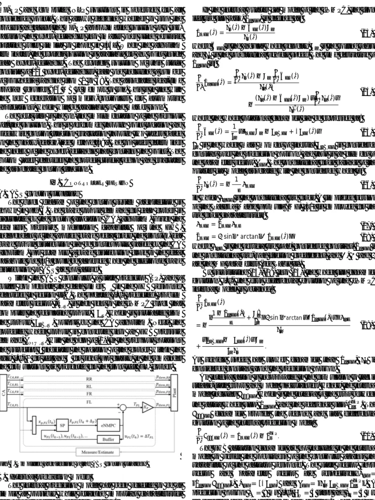
The block diagram of the control system architecture is shown in Fig. 6. The brake torque demand for each corner is calculated by the control allocation (CA) algorithm. Given the seamless pressure modulation capability of the EHB, independent of the applied brake pedal force, the front-to-rear brake torque distribution can be continuously varied by the CA algorithm. For example, a brake distribution close to the ideal parabolic one [40] could be achieved when the electronic brake distribution or ABS are not active.
Within the ABS controller, a state predictor (SP) and a buffer compensate the dead times Δ in the EHB response, identified in section II.C. The updated (i.e., predicted) problem parameters vector, , , is then sent to the eNMPC block that
computes the regulating torque, ∆ , which is subtracted from the torque, , , output by the CA algorithm. Next, the
corrected wheel torque is converted into an EHB pressure demand, , , with the help of (1). In the previous notations
the subscript indicates the location of the corner within the axle, i.e., for left and for right. For clarity, in the remainder the formulations are presented for the front left (FL) corner.
Fig. 6. Simplified architecture of the ABS control strategy.
B. Internal prediction model
The internal prediction model has been selected to be as simple as possible, while retaining important characteristics such a nonlinear tire model formulation.
In the internal quarter car model of the eNMPC, the front left tire slip ratio, , , is defined as:
, ( ) =
( )− ( )
( ) (13)
where is the angular wheel velocity, is the rolling radius and is the longitudinal vehicle speed. The time derivative of
, is: , ( ) = ( )− ( ) ( ) − ( ( )− ( ) ) ( ) ( )
(14)
where the wheel rotational dynamics can be expressed as:
( ) = 1 , − , +∆ ( ) (15)
is the wheel mass moment of inertia. , is considered
constant over the prediction horizon, and thus is an element of the parameter vector, . The longitudinal force balance of the quarter car model associated with the considered wheel is:
( ) =− 1 , (16)
in which , is the longitudinal tire force. A simplified version
of the Pacejka Magic Formula (MF) [31] is employed for the tire force characteristics:
, = , , (17)
, = sin arctan , ( ) (18)
where , is the vertical tire load, considered constant. , is
the longitudinal tire-road friction coefficient, and , and are the MF parameters (see Table II).
By substituting (15)-(18) into (14), the wheel slip dynamics equation, i.e., the first differential equation of the eNMPC internal model, is obtained:
, ( ) =− 1− , ( )+ sin arctan , ( ) , + , − Δ ( ) . (19)
As vehicle speed has slower dynamics than , , is
considered constant along the prediction horizon.
An integral action is incorporated in the formulation to tackle steady-state errors and model uncertainties. Hence, the internal model includes , , which is the integral of the error between
the actual wheel slip, , , and the reference slip, . The , dynamics provide the second and last differential
equation of the internal prediction model:
, ( ) = , ( )− . (20)
The EHB actuation dynamics are not included in the internal model to verify the robustness of the controller against the variability of the actuator response. The state vector, input vector and parameter vector are respectively =
, , , , = [∆ ] and = , , , . A
prediction horizon = 9 ms (i.e., = 3 steps and = 3 ms) is selected for the current implementation. The problem
includes 5 parameters (5-dimensional problem), i.e.,
, ( ) = [ , ( ), , ( ), ( ), , ( ),
( )], and 4 decision variables, i.e., =
[ ( ), ( ), ( ), , ( )]. , is the
slip ratio slack variable. The control horizon is equal to . Longer horizons were also considered in this study and tested in simulation. The final selection was based on the tracking performance of the controller (i.e., the RMS value of the slip ratio error) and the vehicle deceleration profile, which resulted better for = 9 ms.
TABLE II. eNMPC INTERNAL MODEL PARAMETERS.
Symbol Description Value Unit
Apparent front (rear) corner mass 750 (250) kg Wheel rolling radius 0.363 m Wheel mass moment of inertia 2.21 kgm² MF coefficient: stiffness factor 40 - MF coefficient: shape factor 1.4 - MF coefficient: peak value 0.45 - , Front (rear) tire vertical load 7356 (2453) N Table II reports the values of the internal model parameters. The apparent front and rear corner masses have been defined to obtain the same deceleration for the four quarter car models for specific operating conditions, i.e., the 75/25 front-to-rear mass ratio corresponds to the ideal braking distribution ratio for a longitudinal vehicle deceleration of 6 m/s2. Constant values are used for all braking tests.
C. Optimal ABS control problem formulation
The continuous form of the cost function to be minimized during the off-line optimization process is:
= , ( )− ( ) + , ( ) + ∆ ( ) + , ( ) + , − ( ) + , (21) where = 5, = 60, = 10, = 10, = 5 and =
60 are the weights for the different terms, and = 0.1,
= 0.1, = 3000 and = 0.5 are the scaling factors. As a consequence, a tracking problem is set for the first state,
, , and a regulating problem is set for the second state,
, .
The minimization of (21) is subject to the following state and input bound constraints:
λ , − , ( )≤ , ( )≤ , + , ( ) (22)
Δ ≤ ∆ ( )≤ Δ (23)
where Δ = , and Δ = 0, while , and ,
are used as tuning parameters.
D. ABS explicit solution
Fig. 7 is a graphic representation of the 5-dimensional explicit solution computed off-line. Three out of the five parameters are fixed for ease of visualization. In particular, the normalized value of the integral of the slip error, , (2), is set
to 0; the normalized value of vehicle speed, , (3), is set to a
value corresponding to 90 km/h; and the normalized value of
the reference slip ratio, , (5), is set to a value corresponding
to 0.07. Each normalization is performed through characteristic values for the specific application.
The figure reports the normalized control variable, , for a combination of the normalized values of slip ratio, , (1),
and torque demand from the CA algorithm, , (4). Fig. 7 also
indicates the polyhedral regions belonging to different hyper-rectangles, resulting from the generation of the explicit solution.
The control action consists of three main surfaces. Surfaces 1 and 3 represent the upper and lower input constraints described by (23). Surface 2 is the non-saturated control law, which is close to linearity for most of the input parameter values. The red dashed line, indicated as reference in the legend, represents the imposed constant slip reference for this explanatory example.
For small values of , (4), the torque regulation is not
necessary, even for slip ratio values slightly higher than the reference. In fact, in such cases the internal model predicts that the wheel will return to low slip values without intervention. In general, despite the possibility of discontinuities of the explicit solution across the hyper-rectangles, the specific ABS implementation shows significant smoothness of the resulting control action.
Fig. 7. Representation of the explicit solution of the control problem for fixed values of the integral of the slip ratio error, vehicle velocity and reference slip ratio (dashed line). , (1) and , (4) are the normalized input parameters; is the normalized eNMPC control action.
In the on-line implementation, the measured or estimated input parameters would normally be sent directly to the eNMPC. However, given the significance of the identified EHB system dead times, a compensation algorithm is implemented through a concept similar to the one in [22, 41]. A state predictor based on the model formulation presented in section IV.B and a buffer for the past control history predict the parameter trajectory for a horizon length corresponding to the dead time. The inputs to the controller are thus projected into the future, and the control action is evaluated for the final values of this prediction.
With respect to stability, common schemes in the literature for implicit MPC include stabilizing terminal constraints or terminal costs, which need to satisfy Lyapunov-function-type
conditions [42, 43]. Alternatively, [44, 45] present techniques for evaluating stability and performance in NMPC schemes without stability preserving constraints. However, all these approaches are intended for implicit MPC. To the best of the authors’ knowledge, no comparable practical theory is available in the literature to address eNMPC stability. Nevertheless, for this study the control system stability is verified via Monte Carlo simulations, as described in section V.
To assess the computational load due to the evaluation of the eNMPC solution for a comprehensive grid of possible inputs, the controller implementation was initially tested on a dSPACE MicroAutobox II (900 MHz, 16 MB) rapid control prototyping unit, before its installation on the HiL rig. The resulting
computational time was always below 95 μs, which proves that
the eNMPC can run in real-time with virtually any desired time step for the ABS application. For the specific implementation of this study, the time step adopted for the update of the braking torque corrections was 3 ms.
V. ROBUST STABILITY ANALYSIS VIA MONTE CARLO SIMULATIONS
To ensure that the controller is stable and provides good performance for widely varying conditions of the real system, the eNMPC strategy was tested on a large number of challenging scenarios by conducting a Monte Carlo analysis. To do so, the IPG CarMaker model used for the vehicle plant in the HiL setup (see section II.B) was employed in a software-in-the-loop (SiL) fashion. The actuators dynamics and pure time delays were included in the model and parametrized based on the measurements presented in Fig. 4. Similarly to section VI, starting from a constant speed, straight line braking maneuvers with ABS intervention were simulated.
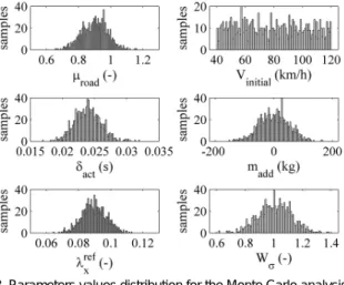
For the generation of the Monte Carlo test scenarios, six critical parameters were varied: i) the initial speed of the braking maneuver, , ; ii) the friction coefficient of the road,
; iii) the vehicle mass (by adding mass, , to the unladen vehicle mass); iv) the pure time delays, Δ, of the EHB system at the four vehicle corners; v) the reference slip ratio for ABS control, ; and vi) the scaling factor, , of the longitudinal tire force relaxation length. The Monte Carlo analysis included 1000 test scenarios, defined by the combination of randomly chosen values of the parameters, each of them possessing a specific probability distribution. Fig. 8a-d show the distribution of the considered values for the six parameters. This was created by assuming that: i) the variation of the initial speed follows a uniform distribution between an upper bound and a lower bound; and ii) the tire-road road friction coefficient, the additional mass, the pure time delay, the reference slip ratio and the relaxation length scaling factor have a normal distribution, which has been tuned to fulfil realistic bounds.
TABLE III. Monte Carlo analysis results.
Test ID Number of simulated scenarios
,% Instability rate**
A* 1000 10% 0%
B 1000 5% 1.3%
* Analysis requirement
** Percentage of total scenarios where instability was detected
Regarding the controller performance assessment, instability was defined based on the European regulation for vehicles equipped with ABS [46], which states that only brief periods of
wheel locking are allowed. Hence, controller instability was considered when a locked wheel was detected for a continuous period of time that was greater than a specified percentage threshold, ,%=10%, of the total duration of the ABS
braking maneuver.
Fig. 8. Parameters values distribution for the Monte Carlo analysis. As indicated by the results of the simulated scenarios in Table III, instability conditions (as low as 1.3% of tests) are only observed for ,% = 5%, while the greater threshold yields 0% instability rate. This behavior can be deemed satisfactory as all instability conditions were detected for ,%
< 10%, and mostly in scenarios with low initial speed, which are commonly considered less safety critical. It was also verified that the controller never brings any corner to operate in free-wheeling conditions because of excess of ABS regulation. In conclusion, the eNMPC controller can be considered very resilient in terms of robust stability.
VI. EXPERIMENTAL SETUP AND RESULTS
The performance of the eNMPC ABS is assessed by simulating a straight line braking maneuver according to the ISO standard 21994:2007 [47] on the HiL rig (see section II). The maneuver is started from a vehicle speed, , , of 100
km/h, with the transmission set to neutral and the clutch disengaged. Two road friction scenarios are considered, with friction coefficients, , of 0.9 and 0.45.
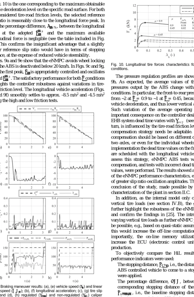
Figs. 9a-d report the eNMPC ABS test results for the high friction scenario, while Figs. 9e-h refer to the low friction conditions. The on-line adaptive identification of the optimal reference slip ratio is not part of this research, which focuses on the preliminary demonstration of eNMPC as feedback control structure for ABS control. Therefore, in Fig. 9 the eNMPC ABS operated without retuning with two reference values of the slip ratio, i.e., 0.07 for the relevant part of the test at = 0.9, and 0.04 for the test at = 0.45. The transition between these values was based on longitudinal vehicle acceleration thresholds, providing a sufficiently good approximation of the available tire-road friction level. The reference slip ratio values, , were computed from the longitudinal tire force characteristics as functions of slip ratio, by using the Pacejka Magic Formula, as reported in Fig. 10. For each front and rear tire, the vertical load at which the longitudinal force characteristic is calculated
in Fig. 10 is the one corresponding to the maximum obtainable vehicle deceleration level on the specific road surface. For both the considered tire-road friction levels, the selected reference slip ratio is reasonably close to the longitudinal force peak. In fact, the percentage difference, , %, between the longitudinal
force at the adopted and the maximum available longitudinal force is negligible (see the table included in Fig. 10). This confirms the insignificant advantage that a slightly higher reference slip ratio would have in terms of stopping distance, at the expense of reduced vehicle steerability.
Figs. 9a and 9e show that the eNMPC avoids wheel locking until the ABS is deactivated below 20 km/h. In Figs. 9c and 9g, after the first peak, is appropriately controlled and oscillates around . The satisfactory performance for both conditions highlights the controller robustness against variations in tire-road friction level. The longitudinal vehicle acceleration (Figs. 9b and 9f) smoothly settles to approx. -8.5 m/s2 and -4.5 m/s2 during the high and low friction tests.
Fig. 9. Braking maneuver results: (a), (e) vehicle speed ( ) and linear wheel speed ( ); (b), (f) longitudinal acceleration; (c), (g) tire slip ratio; and (d), (h) regulated ( ) and non-regulated ( ) caliper pressures. The left column refers to high friction conditions; the right column refers to low friction conditions.
Fig. 10. Longitudinal tire forces characteristics for different braking conditions.
The pressure regulation profiles are shown in Figs. 9d and 9h. As expected, the average values of the front and rear pressures output by the ABS change with the two friction conditions. In particular, the front-to-rear pressure ratio reduces from ~2 at = 0.9 to ~1 at = 0.45, because of the reduced vehicle deceleration, and thus lower vertical axle load transfer. Such variation of the average operating pressure has an important consequence on the controller design. In fact, as the EHB system dead time varies with (see Fig. 4), which, in turn, is influenced by the tire-road friction level, the dead time compensation strategy needs be adaptable. In particular, the compensation should be based on different dead times for the two axles, or even for the individual wheels. In the proposed implementation the dead time values on the front and rear axles are scheduled with the longitudinal vehicle deceleration. To assess this strategy, eNMPC ABS tests without dead time compensation, and tests with incorrect dead time compensation values, were performed. The results showed a significant decay of the eNMPC performance characteristics, especially in terms of greater slip ratio oscillation amplitudes. This is an important conclusion of the study, made possible by the experimental characterization of the plant in section II.C.
In addition, as the internal model only considers constant vertical tire loads (see section IV.B), the good HiL results further highlight the robustness of the eNMPC ABS approach and confirm the findings in [25]. The introduction of time-varying vertical tire loads as further eNMPC parameters would be possible, e.g., based on quasi-static assumptions. However, this would increase the off-line computation time and, more importantly, the on-line memory utilization, which may increase the ECU (electronic control unit) cost in series production.
To objectively compare the HiL results, the following performance indicators were used:
The stopping distance, , i.e., the distance covered by the ABS controlled vehicle to come to a stop after the brakes were applied.
The percentage difference, , between and the corresponding stopping distance of the passive vehicle, , i.e., the baseline stopping distance with locked wheels measured during HiL braking tests for the vehicle without ABS:
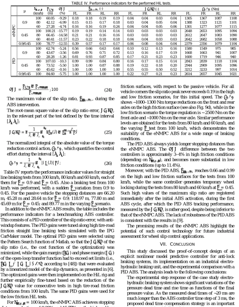
TABLE IV. Performance indicators for the performed HiL tests. µ , (km/h) (m) (%) , (-) (-) (Nm) FL FR RL RR FL FR RL RR FL FR RL RR eN M P C 0.9 100 60.05 -9.29 0.18 0.18 0.19 0.19 0.04 0.04 0.03 0.04 1305 1367 1087 1108 80 42.12 -6.99 0.15 0.15 0.17 0.18 0.03 0.04 0.05 0.04 1388 1323 1121 1101 60 27.28 -4.74 0.16 0.16 0.19 0.24 0.04 0.04 0.05 0.06 1301 1277 1077 1115 0.45 100 100.21 -15.77 0.19 0.19 0.14 0.14 0.03 0.03 0.03 0.03 2648 2653 1095 1094 80 66.45 -14.58 0.21 0.21 0.16 0.16 0.03 0.03 0.03 0.03 2612 2647 1083 1090 60 40.41 -11.57 0.23 0.22 0.18 0.18 0.04 0.04 0.03 0.03 2642 2682 1058 1088 0.9/0.45 100 78.77 -12.55 0.39 0.57 0.17 0.17 0.06 0.08 0.04 0.04 2379 2356 1079 1104 P ID 0.9 100 62.74 -5.24 0.56 0.66 0.63 0.64 0.10 0.12 0.13 0.16 1580 1549 975 985 80 43.67 -3.56 0.69 0.76 0.71 0.72 0.13 0.16 0.17 0.19 1668 1663 941 1007 60 28.28 -1.26 0.81 0.93 0.87 0.85 0.17 0.21 0.23 0.23 1600 1719 946 940 0.45 100 107.03 -10.3 0.99 0.99 0.84 0.80 0.16 0.17 0.15 0.14 2843 2839 1118 1104 80 73.52 -5.50 1.00 1.00 0.87 0.88 0.19 0.22 0.18 0.20 2944 2909 1095 1096 60 45.62 -0.16 1.00 1.00 1.00 1.00 0.55 0.55 0.50 0.52 3212 3233 997 1014 0.9/0.45 100 84.60 -5.75 1.00 1.00 1.00 1.00 0.22 0.27 0.21 0.23 2614 2657 1045 1021 = − ∙100 (24)
The maximum value of the slip ratio, , , during the
ABS intervention.
The root-mean square value of the slip ratio error, , in the relevant part of the test defined by the time interval
[ , ]:
= 1
− ( )− (25)
The normalized integral of the absolute value of the torque reduction control action, , which quantifies the control effort during the interval [ , ]:
= 1
− |∆ ( )| ; (26)
Table IV reports the performance indicator values for straight line braking tests from 100 km/h, 80 km/h and 60 km/h, each of them for = 0.9 and = 0.45. Also a braking test from 100 km/h was performed, with a sudden variation from 0.9 to 0.45. For the passive vehicle the stopping distances are 66.20 m, 45.28 m and 28.64 m for = 0.9; 118.97 m, 77.80 m and 45.69 m for = 0.45; and 89.77 m in the varying scenario.
In addition to the eNMPC ABS results, the table includes the performance indicators for a benchmarking ABS controller. This consists of a PID controller of the slip ratio error, with anti-windup features. The PID gains were tuned along high tire-road friction straight line braking tests simulated with the IPG CarMaker model. The optimal PID gains were selected using the Pattern Search function of Matlab, so that the of the slip ratio (i.e., the cost function of the optimization) was minimized, while the gain margin ( ) and phase margin ( ) of the open-loop transfer function had to exceed set limits (i.e.,
≥ 2, ≥ 30 deg, according to [48]) that were evaluated
by a linearized model of the slip dynamics, as presented in [6]. The optimized gains were then implemented on the HiL rig and further empirically fine-tuned based on the reduction of the value for consecutive tests in high tire-road friction conditions from 100 km/h. The same PID gains were used for the low friction HiL tests.
For , = 100 km/h, the eNMPC ABS achieves stopping
distance reductions of 9.29% and 15.77% on the high and low
friction surfaces, with respect to the passive vehicle. For all vehicle corners the slip ratio peak never exceeds 0.19 in the high and low friction scenarios, for this initial speed. The shows ~1000–1300 Nm torque reductions on the front and rear axles on the high friction surface (see also Fig. 9d), while in the low friction scenario the torque regulation is ~ 2500 Nm on the front axle and ~1000 Nm on the rear axle. Similar performance levels are obtained for the tests from 80 km/h and 60 km/h, and the varying test from 100 km/h, which demonstrates the suitability of the eNMPC ABS for a wide range of braking conditions.
The PID ABS always yields longer stopping distances than the eNMPC ABS. The difference between the two controllers is approximately 3–4% in high friction conditions (depending on , ), and becomes more substantial in low
friction conditions (up to 11.4%).
Moreover, with the PID ABS, , reaches 0.66 and 0.99
on the high and low friction surfaces for the tests from 100 km/h, while the same controller generates temporary wheel locking during the tests from 80 km/h and 60 km/h at = 0.45. Such high values of the maximum slip ratio are registered immediately after the initial ABS activation, during the first ABS cycle, after which the PID ABS tracking performance, measured by the , is rather good, despite being inferior to that of the eNMPC ABS. The lack of robustness of the PID ABS is consistent with the results in [9].
The promising results of the eNMPC ABS highlight the potential of such control technology for future industrial assessment for wheel slip control applications.
VII. CONCLUSION
This study discussed the proof-of-concept design of an explicit nonlinear model predictive controller for anti-lock braking systems, its implementation on an industrial electro-hydraulic braking unit, and the experimental comparison with a PID ABS. The analysis leads to the following conclusions: The experimental step response of the case study
electro-hydraulic braking system shows significant variations of the pressure dead time and rise time as functions of the final pressure value. As the measured dead times of ~20 ms are much longer than the ABS controller time step of 3 ms, the proposed dead time compensation strategy is an important component of the eNMPC ABS.
The experimental braking test results show the eNMPC robustness with respect to the tire-road friction conditions and initial speed. Satisfactory performance was obtained with a relatively simple internal model formulation that did not consider actuation dynamics nor vertical tire load variation. Conversely, the dead time compensation strategy was necessary to ensure the correct performance of the controller.
The on-line computation time for the explicit solution was assessed on an automotive rapid control prototyping unit to be < 95 μs, which confirms the real-time capability of the eNMPC ABS for any implementation time step typical of ABS applications. The memory requirements are also in-line with available automotive micro-controller units (up to 16 MB).
The eNMPC ABS consistently outperforms the PID ABS, e.g., it reduces the stopping distance in low tire-road friction conditions by up to 11.4%. These results make eNMPC a promising technology for automotive wheel slip control applications.
REFERENCES
[1] Z. Tianjun and Z. Changfu, “Research on electro-hydraulic brake system for vehicle stability,” Int. Conf. Ind. Inf. Syst. IIS 2009, pp. 344–347, 2009. [2] E. Nakamura, M. Soga, A. Sakai and T. Kobayashi, “Development of Electronically Controlled Brake System for Hybrid Vehicle,” SAE Technical Paper, 2002.
[3] V. Ivanov, D. Savitski and B. Shyrokau, “A Survey of Traction Control and Anti-lock Braking Systems of Full Electric Vehicles with Individually-Controlled Electric Motors,” IEEE Trans. Veh. Technol., vol. 64, no. 9, pp. 3878–3896, 2015.
[4] D. Savitski, V. Ivanov, D. Schleinin, K. Augsburg, T. Pütz and C. F. Lee, “Advanced control functions of decoupled electro-hydraulic brake system,” IEEE 14th Int. Work. Adv. Motion Control. AMC 2016, pp. 310– 317, 2016.
[5] N. D’Alfio, A. Morgando and A. Sorniotti, “Electro-hydraulic brake system: design and test through hardware-the-loop simulation,” Veh. Syst. Dyn., vol. 44, sup. 1, pp. 378–392, 2006.
[6] M.S. Savaresi and M. Tanelli, Active Braking Control System Design for Vehicles, Springer, 2010.
[7] A.A. Aly, E.-S. Zeidan, A. Hamed and F. Salem, “An Antilock-Braking Systems (ABS) Control: A Technical Review,” Intell. Control Autom., vol. 2, no. 3, pp. 186–195, 2011.
[8] S.B. Choi, “Antilock Brake System with a Continuous Wheel Slip Control to Maximize the Braking Performance and the Ride Quality,” IEEE Trans. Control Syst. Technol., vol. 16, no. 5, pp. 996–1003, 2008.
[9] D. Savitski, D. Schleinin, V. Ivanov and K. Augsburg, “Robust Continuous Wheel Slip Control with Reference Adaptation: Application to Brake System with Decoupled Architecture,” IEEE Trans. Ind. Inf., 2018 (in press).
[10] S. De Pinto, C. Chatzikomis, A. Sorniotti and G. Mantriota, “Comparison of Traction Controllers for Electric Vehicles with On-Board Drivetrains,” IEEE Trans. Veh. Technol., vol. 66, no. 8, pp. 6715-27, 2017.
[11] V.R. Aparow, F. Ahmad, K. Hudha and H. Jamaluddin, “Modelling and PID control of antilock braking system with wheel slip reduction to improve braking performance,” Int. J. Veh. Saf., vol. 6, no. 3, p. 265-296, 2013.
[12] M. Amodeo, A. Ferrara, R. Terzaghi and C. Vecchio, “Wheel slip control via second-order sliding-mode generation,” IEEE Trans. Intell. Transp. Syst., vol. 11, no. 1, pp. 122–131, 2010.
[13] D. Yin, S. Oh and Y. Hori, “A novel traction control for EV based on maximum transmissible torque estimation,” IEEE Trans. Ind. Electron., vol. 56, no. 6, pp. 2086–2094, 2009.
[14] H. Fujimoto, J. Amada and K. Maeda, “Review of traction and braking
control for electric vehicle,” IEEE Veh. Power and Propulsion Conf. VPPC
2012, pp. 1292-1299, 2012.
[15] Y. Wang, H. Fujimoto and S. Hara, “Driving force distribution and control
for EV with four in-wheel motors: A case study of acceleration on
split-friction surfaces,” IEEE Trans. Ind. Electron., vol. 64, no. 4, pp.3380-3388,
2017.
[16] T.A. Johansen, I. Petersen, J. Kalkkuhl and J. Ludemann, “Gain-scheduled wheel slip control in automotive brake systems,” IEEE Trans. Control Syst. Technol., vol. 11, no. 6, pp. 799–811, 2003.
[17] C. Satzger, R. De Castro, A. Knoblach and J. Brembeck, “Design and validation of an MPC-based torque blending and wheel slip control strategy,” IEEE Intell. Veh. Symp. Proc., vol. 2016–August, no. iv, pp. 514–520, 2016.
[18] C. Satzger and R. De Castro, “Combined wheel-slip control and torque blending using MPC,” Int. Conf. Connect. Veh. Expo, ICCVE 2014 - Proc., pp. 618–624, 2014.
[19] R. De Castro, R.E. Araújo, M. Tanelli and S.M. Savaresi, “Torque blending and wheel slip control in EVs with in-wheel motors,” Veh. Syst. Dyn., vol. 50, supp. no. 1, pp. 71–94, 2012.
[20] C. Satzger and R. De Castro, “Predictive Brake Control for Electric Vehicles,” IEEE Trans. Veh. Technol, vol. 67, no. 2, pp. 977-990, 2018. [21] D. Yoo and L. Wang, “Model based wheel slip control via constrained
optimal algorithm,” IEEEInt. Conf. Control Appl., CCA 2007, pp. 1239-1246, 2007.
[22] F. Borrelli, A. Bemporad, M. Fodor and D. Hrovat, “An MPC/hybrid system approach to traction control,” IEEE Trans. Control Syst. Technol., vol. 14, no. 3, pp. 541–552, 2006.
[23] M.S. Basrah, E. Siampis, E. Velenis, D. Cao and S. Longo, “Wheel slip control with torque blending using linear and nonlinear model predictive control,” Veh. Syst. Dyn., vol. 55, no. 11, pp. 1665–1685, 2017.
[24] L. Yuan, H. Zhao, H. Chen and B. Ren, “Nonlinear MPC-based slip control for electric vehicles with vehicle safety constraints,” Mechatronics, vol. 38, pp. 1–15, 2016.
[25] D. Tavernini, M. Metzler, P. Gruber and A. Sorniotti, “Explicit Nonlinear Model Predictive Control for Electric Vehicle Traction Control,” IEEE Trans. on Contr. Syst. Technol., 2018 (in press).
[26] A. Bemporad, D. Bernardini, R. Long, and J. Verdejo, “Model Predictive Control of Turbocharged Gasoline Engines for Mass Production,” SAE Technical Paper, 2018.
[27] E. Siampis, E. Velenis, S. Gariuolo, and S. Longo, “A Real-Time Nonlinear Model Predictive Control Strategy for Stabilization of an Electric Vehicle at the Limits of Handling,” IEEE Trans. Control Syst. Technol., vol. 26, no. 6, pp. 1982-1994, 2018.
[28] B.J. Ganzel, “Slip control boost braking system,” US Patent No. 9,221,443 B2, 2015.
[29] L. De Novellis, A. Sorniotti, P. Gruber, J. Orus, J. M. Rodriguez Fortun, J. Theunissen and J. De Smet, “Direct yaw moment control actuated through electric drivetrains and friction brakes: Theoretical design and experimental assessment,” Mechatronics, vol. 26, pp. 1-15, 2015. [30] D. Savitski, "Robust Control of Brake Systems with Decoupled
Architecture," PhD thesis, Technische Universität Ilmenau, 2019. [31] H.B. Pacejka, Tire and Vehicle Dynamics, Butterworth Heinemann, 2012. [32] E. Giangiulio and D. Arosio, “New validated tire model to be used for ABS and VDC simulations,” 3rd Int. Colloquium Veh.-Tyre-Road Interact., pp. 1-17, 2006.
[33] J.A. Grancharova and T.A. Johansen, Explicit nonlinear model predictive control: Theory and applications, Vol. 429. Springer, 2012.
[34] T.A. Johansen, “On multi-parametric nonlinear programming and explicit nonlinear model predictive control,” Proc. 41st IEEE Conf. Decis. Control.
2002., vol. 3, pp. 2768-2773, 2002.
[35] L.F. Domínguez and E.N. Pistikopoulos, “Recent Advances in Explicit Multiparametric Nonlinear Model Predictive Control,” Ind. Eng. Chem. Res., vol. 50, no. 2, pp. 609–619, 2011.
[36] P. Tøndel and T.A. Johansen, “Lateral Vehicle Stabilization Using Constrained Nonlinear Control,” Eur. Control Conf., pp. 1887–1892, 2003. [37] M. Herceg, M. Kvasnica, C.N. Jones and M. Morari, “Multi-parametric
toolbox 3.0,” Eur. Control Conf., pp. 502–510, 2013.
[38] A. Wächter and L.T. Biegler, “On the Implementation of a Primal-Dual Interior Point Filter Line Search Algorithm for Large-Scale Nonlinear Programming,” Math. Program., vol. 106, no. 1, pp. 25–57, 2006. [39] P. Tøndel, T.A. Johansen and A. Bemporad, “Evaluation of piecewise
affine control via binary search tree,” Automatica, vol. 39, no. 5, pp. 945– 950, 2003.
[40] R. Limpert, Brake Design and Safety, Society of Automotive Engineers, 1999.
[41] M. Jalaliyazdi, A. Khajepour, S. Chen and B. Litkouhi, “Handling Delays in Stability Control of Electric Vehicles Using MPC,” SAE Technical Paper, 2015.
Predictive Control Scheme with Guaranteed Stability,” Automatica, vol. 34, no. 10, pp. 1205–1217, 1998.
[43] D.Q. Mayne, J.B. Rawlings, C.V. Rao and P.O.M. Scokaert, “Constrained model predictive control: Stability and optimality,” Automatica, vol. 36, no. 6, pp. 789–814, 2000.
[44] L. Grüne, “Analysis and Design of Unconstrained Nonlinear MPC Schemes for Finite and Infinite Dimensional Systems,” SIAM J. Control Optim., vol. 48, no. 2, pp. 1206–1228, 2009.
[45] M. Reble and F. Allgöwer, “Unconstrained model predictive control and suboptimality estimates for nonlinear continuous-time systems,”
Automatica, vol. 48, no. 8, pp. 1812–1817, 2012.
[46] “Regulation No 13 of the Economic Commission for Europe of the United Nations (UN/ECE) — Uniform provisions concerning the approval of vehicles of categories M, N and O with regard to braking,” Official Journal of the European Union, 2010.
[47] International Standard “Passenger cars - Stopping distance at straight-line braking with ABS - Open-loop test method” Reference number: ISO 21994:2007.
[48] S. Skogestad and I. Postlethwaite, Multivariable feedback control: analysis and design, New York: Wiley, 2007.
Davide Tavernini received the M.Sc. degree
in mechanical engineering and Ph.D. degree in dynamics and design of mechanical systems from the University of Padova, Padua, Italy, in 2010 and 2014. During his Ph.D. he was part of the motorcycle dynamics research group. He is a Lecturer in advanced vehicle engineering with the University of Surrey, Guildford, U.K. His research interests include vehicle dynamics modeling and control, mostly applied to electric and hybrid electric vehicles.
Fabio Vacca received the M.Sc. degree in
mechanical engineering from the Politecnico di Bari, Bari, Italy, in 2013. He is currently pursuing the Ph.D. degree in automotive engineering with the University of Surrey, Guildford, UK. His research interests include hybrid electric vehicles, electric vehicles and vehicle dynamics
Mathias Metzler (GSM’17) received the
Dipl.-Ing. degree in mechanical engineering from Vienna University of Technology, Vienna, Austria, in 2015. He is currently pursuing the Ph.D. degree in advanced vehicle engineering with the University of Surrey, Guildford, U.K. His research interests include vehicle dynamics control, model predictive control, optimization and nonlinear systems.
Dzmitry Savitski (S’12–M’18) received the
Dipl.-Ing. degree in automotive engineering from the Belarusian National Technical University, Minsk, in 2011. From 2011 to 2018, he worked towards the Dr.-Ing. degree in automotive engineering with the Technische Universität Ilmenau (TUIL), Ilmenau, Germany. Dzmitry Savitski is now a Lead Engineer with Arrival Germany GmbH, Pforzheim, Germany, and develops control software for X-by-Wire chassis systems.
Valentin Ivanov (M’13–SM’15) received the
Mech. Eng., Ph.D. and D.Sc. degrees in automotive engineering from the Belarusian National Technical University, Minsk, Belarus, in 1992, 1997 and 2006, and the Dr.-Ing. habil. grade in automotive engineering from the Technische Universität Ilmenau (TUIL), Ilmenau, Germany, in 2017. From 1998 to 2007, he was Assistant Professor, Associate Professor and Full Professor with the Department of Automotive Engineering, Belarusian National Technical University. He is European Project Coordinator with the Automotive Engineering Group at TUIL. His research interests include vehicle dynamics, electric vehicles, automotive control systems and chassis design.
Patrick Gruber received the M.Sc. degree in
motorsport engineering and management from Cranfield University, Cranfield, U.K., in 2005, and the Ph.D. degree in mechanical engineering from the University of Surrey, Guildford, U.K., in 2009. He is a Reader in advanced vehicle systems engineering with the University of Surrey. His research interests include vehicle dynamics and tire dynamics with special focus on friction behavior.
Ahu Ece Hartavi received the M.Sc. and
Ph.D. degrees in electrical engineering from Istanbul Technical University, Istanbul, Turkey, in 2000 and 2006. She is a Senior Lecturer with the University of Surrey, Guildford, U.K. Her research interests include intelligent control, electric vehicle modeling and control, and automated vehicles.
Miguel Dhaens received the M.Sc. degree in
electro-mechanical engineering from KIH, Ostend, Belgium. He is Engineering Manager of the Global Research Ride Performance Team of Tenneco, and responsible for defining the research road map and coordinating the global research activities of Tenneco’s Ride Performance business, which includes vehicle dynamics, damping solutions, mechatronics, material science, manufacturing technologies and predictive tools. Before joining Tenneco, he worked with the Formula One team of Toyota Motorsport GmbH, Germany, as Manager of the engine, testing and advanced strategies teams, and with Flanders Drive as R&D Manager .
Aldo Sorniotti (M’12) received the M.Sc.
degree in mechanical engineering and Ph.D. degree in applied mechanics from the Politecnico di Torino, Turin, Italy, in 2001 and 2005. He is a Professor in advanced vehicle engineering with the University of Surrey, Guildford, U.K., where he coordinates the Centre for Automotive Engineering. His research interests include vehicle dynamics control and transmission systems for electric and hybrid electric vehicles.