Prediction of composite indicators using locally weighted
quantile regression
Jurga Rukš˙enait˙ea, Pranas Vaitkusb, Povilas Asijaviˇciusb
aVilnius Gediminas Technical University,
Saul˙etekio ave. 11, LT-10223 Vilnius, Lithuania [email protected]
b
Vilnius University,
Naugarduko str. 24, LT-03225 Vilnius, Lithuania [email protected]
Received:December 18, 2016 / Revised:November 17, 2017 / Published online:December 14, 2017 Abstract. The main goal of this paper is to improve the existing methods and tools used for solving penalized quantile regression problems. We modified the quantile regression method by implementing the extreme learning machine (ELM) algorithm and features of locally weighted regression. Also, we used different penalty functions. A modified method was used for the one-step-ahead prediction of the composite indicator (CI) of the Lithuanian economy. Our analysis showed that the prediction error of the modified locally weighted quantile regression is smaller in comparison to the other quantile regression.
Keywords: quantile regression, penalty function, extreme learning machine, locally weighted regression, composite indicators.
1
Introduction
Linear regression methods are well known as classical methods; the ordinary least square (OLS) method allows us to assess the linear relationship of variables. This method finds the conditional mean of the response variable. On the other hand, the OLS method is very sensitive to outliers; hence, it provides unstable estimates. Also applicable is the LADR (least absolute deviation regression), which evaluates the median of the response variable. The median is more robust to outliers; hence, this method is more robust to outliers as well. LADR was summarized in [4] when developing the quantile regression. In this way, the conditional quantile of any order was obtained; practically, this fact characterizes the conditional distribution of a response variable. Over the past thirty-five years, quantile regression has become a very important and widely used technique to analyze the whole conditional distribution of a response variable. Such methods are more robust to outliers than that of the linear regression.
The first step of any regression modeling is the selection of variables. In practical problems, there are situations where quite a few variables are important. Usually, most
of them are included in the model, and only then are the most important ones chosen. Insignificant variables should not be included in the model since they complicate in-terpretation of results and reduce the accuracy of predictions. In order to automate this process, the regularization of the method is often applied. Many versions of regularization are proposed. The L1 regularization is used in the LASSO (least absolute shrinking and selection operator) method [11]. Later, the LASSO method was improved into the adaptive LASSO method [13]. The nonconcave penalized least squares regression was introduced [2]. This method selects the significant variables and evaluates the estimates of coefficients simultaneously. An example of such a function is SCAD (smoothly clipped absolute deviation) regularization. Also, logarithmic and exponential regularizations were introduced. Later, the MCP (minimax concave penalty) function was developed [12]. In most cases, these above-mentioned penalty functions were used in solving linear regres-sion problems, yet almost analogous methods can be used in quantile regresregres-sion methods. This work is an extension of previous work, where the ELM algorithm was combined with the locally weighted regression for the one-step-ahead prediction of the compos-ite indicator (CI) of the Lithuanian economy [8]. An analysis of results showed that the combined method gives a smaller prediction error in comparison to the Levenberg– Marquard, ELM methods or AR(p) process. Also, the analysis of the results based on various accuracy measures suggested that the proposed method may be used for data of rather small sample size and during periods when dynamics of time series may have unexpected changes like during the economical crises and later periods (2008–2010). In spite of the acceptable results, as mentioned in the beginning of the paper, it is known that the OLS method is sensitive to outliers. Hence, the quantile regression was chosen as an alternative (that is, more robust to outliers) for the one-step-ahead prediction of CI.
In practical examples, we will use the CI of the Lithuanian economy that was devel-oped under the methodology described in [7]. The methodology for constructing the CI is based on factor analysis. In this paper, the practical problems of quantile regression are solved using the R packagerqPen[9]. In this package, different regularization functions are implemented: LASSO, SCAD, and MCP. This tool enables us to solve quantile regression problems using these above-mentioned regularization functions.
The general objective of this research is to modify the existing quantile regression: (i) to develop the locally weighted quantile regression using different regularization func-tions and the ELM method for the modification of input data; (ii) to check the impact of different regularization functions on the predicted results of CI’s.
The structure of this paper is as follows: In Section 1, methodological notes are intro-duced. The practical implementation of the methods is described in Section 3. Section 4 describes the results, and Section 5 gives concluding remarks.
2
Methodology
In this section, we define our main terms and introduce the methods used in this paper: the quantile regression with regularization, regularization functions, the locally weighted quantile regression, and the locally weighted quantile regression with the ELM modifica-tion.
2.1 Quantile regression with regularization
Suppose we have the random variables (r.v.)Y andX. Also suppose theY’s distribution function with the condition thatX =xisFY(y|X =x) =P(Y 6y |X =x). Then
Y’sτ ∈[0,1]order quantile with conditionX =xis defined as a number: QY|X(τ) =FY−1(τ|X=x) = inf
y: FY(y|X=x)>τ .
Functionfτ(x)is called theτth order (where0< τ <1) quantile function if:P(Y <
fτ(x)|X) =τ.
We define ther=y−fτ(x|β), then the “check” function:
ρτ(r) =
(
τ r ifr >0,
−(1−τ)r otherwise. (1)
Such a “check” function (1) can be used for the evaluation of the quantiles of r.v. Suppose that Y is r.v. with distribution function FY(y) = P(Y 6 y). Then the
quantile ofτorder is equal
QY(τ) = argmin
u E ρτ(Y −u)
.
Having the realizationy1. . . , yN of r.v.Y, we evaluate the estimate ofτorder quantile
of r.v.Y: b QY(τ) = argmin u ( 1 N N X i=1 ρτ(yi−u) ) = argmin u ( 1 N N X i=1 τ(yi−u)I(yi> u) + (1−τ)(u−yi)I(yi6u) ) = argmin u Eb ρτ(Y −u) .
Moving to the quantile regression, suppose the argumentuis dependent on the r.v.X, i.e.,u=fτ(X). Then we find theY’s conditional quantileQY|X(τ)of orderτ.
Analogically, if we have realizations {(xi, yi), i = 1, . . . , N}, where xi = (xi1,
. . . , xip), we can solve the regression problem between Y and X using the “check”
function (1). In this case, we will get the estimateQbY|X(τ)ofτorder conditional quantile
of the response variable. In another way, we have this minimization problem:
min fτ N X i=1 ρτ yi−fτ(xi|β) . (2)
When similar minimization problems are solved, regularization method is often used. Often, the regularization functionsL1andL2are used. Then we obtain the LASSO and ridge regression.
Hence, in order to get better results for the quantile regression problem, we shall add the penalty functionJ(fτ):
min fτ N X i=1 ρτ yi−fτ(xi|β)+λJ(fτ), (3)
hereβ= (β1, . . . ,βp), and the regularization parameterλis carefully chosen.
2.2 Regularization functions
The regularization technique permits us to choose only significant variables for the re-gression; also, it helps us avoid overfitting. In this paper, we analyzed three different techniques: LASSO, SCAD, MPC.
LASSO method was defined in order to improve the OLS method [11]. Formerly, two main approaches were employed: ridge regression and the exclusion of insignificant variables from the model. Ridge regression gives fewer estimates of stabler coefficients. The second approach rejects irrelevant covariates and makes the results easier to interpret. LASSO combines features of both methods; hence, this method has its drawbacks. The LASSO regularization function shall be defined:
J(fτ) =λJ(β) =λ p X j=1 |βj|, herePp
j=1|βj|6t,tis a parameter that controls the shrinkage of coefficients.
SCAD function was defined in [2]. This regularization function is symmetric and nonconcaved on the interval(0,∞):
pλ(βj) = λ|βj| if|βj|6λ, −(|βj|2−2aλ|βj|+λ2 2(a−1) ) ifλ <|βj|6aλ, (a+1)λ2 2 if|βj|> aλ.
Hence, the SCAD regularization function is differentiable in the interval(−∞,0)∪ (0,+∞), but its derivative outside of the interval[−aλ, aλ]is equal to zero. SCAD should give unbiased estimates of coefficients and exclude insignificant variables.
In [2], there is a recommendation to useα= 3.7, whileλis often chosen by cross-validation or other methods.
MCP functioncan be used in solving linear regression problems. The estimates ob-tained using MCP are accurate and almost unbiased. This algorithm can be used in solving the large dimension multiple regression [12]. MCP regularization can be defined:
p(t;λ) =λ |t| Z 0 1− x γλ + dx= λ|t| − t 2 2γ I |t|< λγ +λ 2γ 2 I |t|>λγ ,
Regularization function p(t;λ) with parameter t is nonincreasing in the interval
(−∞,0)and nondecreasing in the interval (0,∞), its derivative p(t;λ)0tis continuous
in the above-mentioned intervals.
2.3 Locally weighted quantile regression
The goal of the regression is to evaluate the functionminE(Y |X) =m(X)having the response variableY and independent variableX.
In the linear dependency betweenY andX and having realization of these random variables{(xi, yi), i= 1, . . . , N}, the linear regression is defined asyi=βTxi+i, here
β= (β1, . . . , βp)T,xi = (xi1, . . . xip)Tandiis error. In this case,yi =m(xi) +i,
wherem(xi) =β1xi1+· · ·+βpxip. Coefficientsβ1, . . . , βp will be evaluated solving
the minimization problem
min β N X i=1 yi−βTxi 2 . (4)
In general, the results of such a minimization may be improved. The regression results obtained are usually applied to evaluate the prediction regarding the latest values of the independent variableyˆN+1 = βT(xN+1). If xN+1 is different from otherxi, theβT
obtained may be insufficiently accurate.
Hence, in this paper, the locally weighted regression shall be used [5]. It modifies expression (4), which gives weights to the errorsωi:
min β N X i=1 ωi yi−βTxi 2 .
For locally weighted regression, the weightsωi are determined depending on how
“close” xi is to the new query xq (further xq = xN+1). Often, the Gaussian kernel
functionKis used: K(xi,xq) = exp −kxi−xqk 2 2σ2 , kxi−xqk2= q (xi−xq)2, whereσ2∈Ris arbitrary.
We select the ωi = K(xi,xq). K(xn,x0) → 1 when kxn −x0k → 0, and
K(xn,x0)→0whenkxn−x0k → ∞. Finally, we obtain this optimization problem:
min ˜ β N X i=1 K(xi,xq) yi−β˜Txi 2 , (5)
hereβ˜ = ( ˜β1, . . . ,β˜p)T. The solution to this problem is similar not very different from
that of problem (4). Expression (5) is transformed:
min ˜ β N X i=1 K(xi,xq)1/2yi−K(xi,xq)1/2β˜Txi 2 = min ˜ β N X i=1 K(xi,xq)1/2yi− p X j=1 ˜ βjK(xi,xq)1/2xij !2 = min ˜ β N X i=1 zi− p X j=1 ˜ βjξij !2 , herezi=K(xi,xq)1/2yiandξij =K(xi,xq)1/2xij,i= 1, . . . , N,j= 1, . . . , p.
Analogically, we solve the quantile regression problem. Suppose, we have a quantile regression without regularization:
min fτ N X i=1 ωiρτ yi−fτ(xi |β) = min fτ N X i=1 K(xi,xq)ρτ yi−fτ(xi|β) . (6)
After certain transformations, we note: fτ(xi|β) = β1xi1+· · ·+βpxip =βTxi,
˜
yi = K(xi,xq)yi,x˜i = K(xi,xq)xi. In the case of a linear regression whereωi =
K(xi,xq), we find that the solution of (6) is equivalent to the problem:
min β N X i=1 ρτ y˜i−βTx˜i. (7)
Hence, the locally weighted regression method is reduced to problem (7). This modi-fication gives a more accurate estimate ofβ; in this way, we get a more accurate prediction of the response variable.
2.4 Locally weighted quantile regression with ELM modification
ELM is a widely used method based on the idea of a single hidden layer of feed-forward neural networks (SLFNs) [3, 10].
In our case, ELM is used for the modification of independent variables. Dataxiwill
be changed to a linear transformation with random weights [3], and the activation function (sigmoid function) will be chosen. Let us define the linear quantile regression problem:
min β N X i=1 ρτ yi−βTxi .
Hence, once we havexi, the new pseudovariablesziare created:
zij =ϕ ωjTxi
hereωj = (ω1j, . . . , ωpj)T are randomly generated weights by ELM,ϕ is a sigmoid
function thatϕ(u) =ϕ1(u)orϕ(u) =ϕ2(u), whereϕ1andϕ2are defined: ϕ1:R→[0, M]such thatϕ1(u) =M/(1 + e−hu), hereh >0is a parameter.
ϕ2:R→[−M, M]such thatϕ2(u) =M(eu−e−u)/(eu+ e−u).
We have modified datazi = (zi1, . . . , zim),i= 1, . . . , N. Now, we have themnew
covariates composed of previouspcovariates. The numbermis arbitrary. Exactly these new data will be used in further analysis.
The following formula defines the modified quantile regression:
min β N X i=1 ρτ y˜i−βTx˜i +λJ(β), (9)
here, the response variable is unchanged:
˜
yi=K(xi,xq)yi. (10)
However, we have a new expression of independent variables:
˜
xi=K(xi,xq)zi, (11)
herezi is defined as (8). In this way (only data transformation), the local quantile
re-gression with ELM modified covariates is obtained. The assessment of this method is the same as for the initial quantile regression (2).
3
Practical implementation
In this section, previously described methods will be applied for data analysis. The regres-sion will be constructed in two ways: the general quantile regresregres-sion and locally weighted quantile regression with ELM modified covariates (further – the modified method).
Practical modeling is concentrated on three different values of the order τ (τ = 0.05,0.5,0.95). When the variant isτ = 0.5, we deal with the conditional median of the response variable. As we know, the median and mean are the same for the r.v. with a symmetric density function. The quantile of theτ= 0.5order is the most likely value of the response variable. An interpretation of the quantiles of orderτ = 0.05andτ= 0.95
gives the confidence interval of the response variable (in this case, 90 per cent).
Recently, new indicators (indexes) have been constructed that reflect the changes in economy more precisely than the gross domestic product [8]. Usually, this type of indica-tor is constructed as a combination of different indicaindica-tors from various fields. Statistical data are selected regarding economic theory and additional methods (correlation, causal-ity analysis, etc.). Weights are chosen using mathematical methods or including additional sources of information. In this way, so-called CI’s are constructed. The advantage of the CI mainly depends on the chosen methodology and on selected statistical data that reflect
the general tendencies of a specific field. In summary, the CI is defined as a mathematical function:
CI =f(X,ω),
here, X is a set of variables that compile CI,ω – weights that are assigned to every variable.
In this paper, we will use the methodology for constructing the CI presented in [8]. For the analysis and prediction, we extended the time period (1998–2014) and reduced the number of variables tok = 12. Economical indicators of monthly and quarterly periodicity were used: statistical data of industry, construction, domestic trade, foreign trade, services, the producer price index. We will briefly describe the steps followed in constructing the CI. First of all, a preliminary analysis was applied (outliers were detected, missing values were assigned), and all data were seasonally adjusted. Data of quarterly periodicity were transformed into monthly periodicity. The range of all indicators was transformed into the range [0,1]. Using the factor analysis method, we left only the most important indicators for further analysis. The weights of individual indicators were obtained by using the Nicoletti method [6] from the rotated factor loading matrix.
Hence, we have data{(xt, yt), t= 1, . . . ,204}, wherext = (xt,1, . . . xt,12)is the tvalue of the covariate, andytis thetvalue of CI. Here we changed the indexitotin
order to highlight the importance of time in the time series as the order of data.
In modeling economic indicators, lags of covariates are usually also included in the models. We suppose that
yt=f(xt,xt−1, . . . ,xt−d) +t.
In this case, we say thatydepends on the lastdvalues ofx. In modeling CI, we deal with four different cases. We will use linear dependency and different lags (d= 1,2,3,4):
yt=β0+ d
X
j=1
βjxt−j+t. (12)
We solve problems (12) and obtain the general quantile regression
min β N X t=1 ρτ yt−β0− d X j=1 βjxt−j ! +λJ(β) (13)
and the modified quantile regression method
min β N X t=1 ρτ y˜t−βT˜xt +λJ(β). (14) ˜
yt,x˜tand the components are defined in (8), (10), and (11). Hereβ= (β0, . . . , βd)T, and
J(β)– one of the regularization functions (LASSO, SCAD, or MCP). In methods (13) and (14) withd= 1,2,3,4, CI is evaluated without considering the recent values of the
covariates. Then the modified quantile regression will be constructed “around” the recent value of the covariatext, which will be used in forecasting.
Twelve different models are constructed using the general (3) and modified (9) quan-tile regression by following these steps:
(i) Data points are chosen:1046n6204.
(ii) The lagd(d= 1,2,3,4) and the regularization functionJ(β)are fixed. (iii) Theτorder (τ= 0.05,0.5,0.95) of quantile is chosen.
(iv) The general (3) and the modified (9) quantile regression for thenfirst elements of the sample are used (i.e.,N =n), andxq = (xn, . . . ,xn−d).
(v) Havingxq, we predict (one-step-ahead) the values ofyn of the quantile of the
τorder using the general and modified methods.
(vi) These steps are repeated withτ = 0.05,τ = 0.5, andτ = 0.95. The estimates of the general and modified regressionsyˆn(0.05),yˆn(0.5),yˆn(0.95),yˆˆn(0.05),yˆˆn(0.5), and
ˆ ˆ
yn(0.95)are obtained. The value in brackets stands for the order of the quantile.
This algorithm is repeated with everynfrom the interval[104,204]. E.g., predictions of the modified method:τ = 0.05:ˆy(0.05)= (ˆy(0.05)
104 , . . . ,yˆ (0.05)
204 ), and predictions of the general method are obtained, e.g.,yˆˆ(0.05)= (ˆyˆ104(0.05), . . . ,yˆˆ204(0.05)).
The following measures to verify the accuracy of the models were used:
• Mean absolute error: MAE(ˆy,y) =PT
i=1|yi−yˆi|/T.
• Mean absolute percentage error: MAPE(ˆy,y) =PT
i=1|(yi−yˆi)/yi|/T ·100.
• Root mean square error: RMSE(ˆy,y) = (PT
i=1(yi−yˆi) 2)1/2.
• The measureM1:M1(ˆy,y,ˆˆ y) =PT
i=1I(|ˆyi−yi|<|yˆˆi−yi|)/T. In this case, the M1(ˆy,y,ˆˆ y)indicates the share of all values, where the estimateyˆi is better than
the estimateyˆˆiin comparison to the original datayi.
• The measureM2:M2(ˆy,ˆˆy,y) =P
T
i=1I(ˆyi< yi<yˆˆi)/T. Here, theM2(ˆy,y,ˆˆ y) indicates the share of all values, where the estimate yˆi falls within the interval
betweenˆyandy.ˆˆ
In all formulas,T stands for the length of time series. In practice, we will use theM2 to find out how often the actual value falls within the confidence interval. E.g., for the 90 per cent confidence interval, the measure will be calculated:M2(y(0.05),y(0.95),y), here y(τ)stands for the quantile of theτorder.
4
Results
Finally, after we have performed the modeling with differentdand all regularizations, the set of vectors is obtained:yˆ(0.05),yˆ(0.5),yˆ(0.95),yˆˆ(0.05),yˆˆ(0.5), andyˆˆ(0.95). In order to analyze the accuracy of our predictions, the original data(y104, . . . , y204)are compared to the estimates of quantiles. The prediction value should be around the mean or the median; hence, the prediction of the median shall show the general view. In the case of 90 per cent, the realization of the random variable (CI) should fall within the confidence interval
100 0 .2 0 .4 0 .6 0 .8 1 .0 n C I 0 20 40 60 80
Figure 1.Data with four lags and MCP regularization. (Online version in colour.)
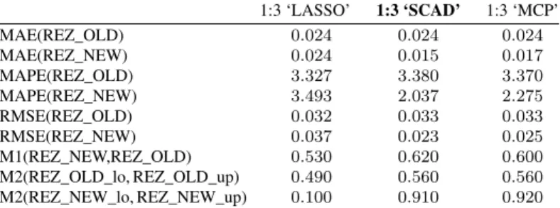
Table 1.Characteristics of accuracy (input data with three lags). 1:3 ‘LASSO’ 1:3 ‘SCAD’ 1:3 ‘MCP’ MAE(REZ_OLD) 0.024 0.024 0.024 MAE(REZ_NEW) 0.024 0.015 0.017 MAPE(REZ_OLD) 3.327 3.380 3.370 MAPE(REZ_NEW) 3.493 2.037 2.275 RMSE(REZ_OLD) 0.032 0.033 0.033 RMSE(REZ_NEW) 0.037 0.023 0.025 M1(REZ_NEW,REZ_OLD) 0.530 0.620 0.600 M2(REZ_OLD_lo, REZ_OLD_up) 0.490 0.560 0.560 M2(REZ_NEW_lo, REZ_NEW_up) 0.100 0.910 0.920
Table 2.Characteristics of accuracy (input data with four lags). 1:4 ‘LASSO’ 1:4 ‘SCAD’ 1:4 ‘MCP’ MAE(REZ_OLD) 0.026 0.027 0.027 MAE(REZ_NEW) 0.017 0.013 0.012 MAPE(REZ_OLD) 3.635 3.763 3.734 MAPE(REZ_NEW) 2.408 1.742 1.635 RMSE(REZ_OLD) 0.036 0.038 0.037 RMSE(REZ_NEW) 0.023 0.018 0.018 M1(REZ_NEW,REZ_OLD) 0.600 0.650 0.680 M2(REZ_OLD_lo, REZ_OLD_up) 0.510 0.460 0.460 M2(REZ_NEW_lo, REZ_NEW_up) 0.090 0.920 0.910
between the0.05and0.95quantiles. Hence, we will analyze how well the model was able to assess the confidence interval of the response variable.
The example (d = 4and MCP regularization) of modeling results is presented in Fig. 1 and in Tables 1, 2. In the figure, the black line denotes the median of original data; the red line denotes the median obtained by the general quantile method; the green line –
by the modified method; the dashed red and green lines denote the0.05and0.95quantiles by the general and modified methods, respectively.
If we observe only the graphical results, it is quite difficult to determine which method is the better one. In different periods, one of the method gives more accurate predictions, or predictions are quite similar.
In the tables, REZ_NEW stands for the estimate of the median obtained by the modi-fied method, and REZ_OLD is the estimate of the median obtained by the general method, REZ_OLD_lo, REZ_OLD_up, REZ_NEW_lo, REZ_NEW_up stand for the quantiles of 0.05 and 0.95, respectively. The notation “1:3” means that input data with the lags first, second, and third were used in a particular model.
Better results were obtained by the modified method using input data with three or four lags. MAE, MAPE, RMSE, and other statistics confirmed this fact. We noticed that the widths of the confidence intervals obtained by both methods are similar, but in the case of the modified method with SCAD and MCP regularizations, more than 90 per cent of observed data fall within the constructed confidence interval. In the case of a general method, only 46 per cent of data realizations fall within the interval. More results can be found in [1].
The analysis showed that measures of accuracy are dependent on regularization and the number of lags. The smallest errors of general method was obtained using LASSO regularization, while in the case of the modified quantile regression, the best result was obtained using four lags and MCP regularization. We see that different methods proceed with different accuracy depending on the number of lags. However, the modified method has this advantage: its confidence interval and estimate of the median are more accurate.
Also, the comparative analysis of obtained results and results of previous research [8] was performed. In this paper and in [8], the CI is slightly different. Here the time period is extended to 1998–2014 (in the previous research, 1998–2010), and the number of vari-ables was reduced tok= 12(previously,k= 28). The purpose and expected results of the combined method of extreme learning machine and locally weighted regression [8] and locally weighted quantile regression are unequal as well. Regardless of the differences we compared some accuracy measures (RMSE and MAPE) of one-step-ahead predictions. The analysis showed that RMSE and MAPE are slightly smaller of best models of locally weighted quantile regression.
5
Conclusions
In this paper, the quantile regression with penalty function was extended by including local weights and the ELM method for the modification of covariates. This developed modified method was adopted for the one-step-ahead prediction of the CI of the Lithua-nian economy. Our analysis indicated that the locally weighted quantile regression with regularization obtains on average better results than the known quantile regression with regularization: the new method enabled us to obtain more accurate conditional medians and predictions of confidence intervals. The best results were obtained by methods with SCAD and MCP regularizations.
References
1. P. Asijaviˇcius, Locally weighted quantile regression, Master thesis, Vilnius University, 2015. 2. J. Fan, R. Li, Variable selection via nonconcave penalized likelihood and its oracle properties,
J. Am. Stat. Assoc.,96(456):1348–1360, 2001.
3. G.-B. Huang, Q.-Y. Zhu, C.-K. Siew, Extreme learning machine: Theory and applications, Neurocomputing,70(1–3):489–501, 2006.
4. R. Koenker, G. Bassett, Regression quantiles, Econometrica,46(1):33–50, 1978.
5. A. Moore, J. Schneider, K. Deng, Efficient locally weighted polynomial regression predictions, in D.H. Fisher (Ed.), Proceedings of the Fourteenth International Conference on Machine Learning, Nashville, TN, July 08–12, 1997, Morgan Kaufmann, San Francisco, CA, 1997, pp. 236–244.
6. G. Nicoletti, S. Scarpetta, O. Boylaud, Summary indicators of product market regulation with an extension to employment protection legislation, OECD Working Papers, No. 226, OECD Publishing, Paris, 2000.
7. J. Rukš˙enait˙e, Impact of factor rotation methods on simulation composite indicators, Math. Model. Anal.,16(3):418–431, 2011.
8. J. Rukš˙enait˙e, P. Vaitkus, Prediction of composite indicators using combined method of extreme learning machine and locally weighted regression, Nonlinear Anal. Model. Control, 17(2):238–251, 2012.
9. B. Sherrwood, Penalized quantile regression, rqPen package documentation, 2015.
10. J. Tang, G. Huang, Extreme learning machine for multilayer perceptron, IEEE Trans. Neural Networks Learn. Syst.,27(4):809–821, 2015.
11. R. Tibshirani, Regression shrinkage and selection via the lasso, J. R. Stat. Soc., Ser. B, 1(58):267–288, 1996.
12. C.H. Zhang, Nearly unbiased variable selection under minimax concave penalty, Ann. Stat., 38(2):894–942, 2010.
13. H. Zou, The adaptive lasso and its oracle properties,J. Am. Stat. Assoc.,101(476):1418–1429, 2006.