Special Issue on Statistics in Biology and Health Sciences 2007, Volume 69, Part 3, pp. 514-547
c
°2007, Indian Statistical Institute
Gene Expression-Based Glioma Classification Using
Hierarchical Bayesian Vector Machines
Sounak Chakraborty
University of Missouri, Columbia, USA
Bani K. Mallick
Texas A & M University, College Station, USA
Debashis Ghosh
University of Michigan, Ann Arbor, USA
Malay Ghosh
University of Florida, Gainesville, USA
Edward Dougherty
Texas A & M University, College Station, USA
Abstract
This paper considers several Bayesian classification methods for the analy-sis of the glioma cancer with microarray data based on reproducing kernel Hilbert space under the multiclass setup. We consider the multinomial logit likelihood as well as the likelihood related to the multiclass Support Vector Machine (SVM) model. It is shown that our proposed Bayesian classification models with multiple shrinkage parameters can produce more accurate clas-sification scheme for the glioma cancer compared to several existing classical methods. We have also proposed a Bayesian variable selection scheme for selecting the differentially expressed genes integrated with our model. This integrated approach improves classifier design by yielding simultaneous gene selection.
AMS (2000)subject classification. Primary 62G08, 62H30, 68T05, 68T10.
Keywords and phrases. Gibbs sampling, Markov chain Monte Carlo, Metro-polis-Hastings algorithm, microarrays, reproducing kernel Hilbert space, shrinkage parameters, support vector machines.
1 Introduction
There are two main types of brain tumours: those that start in the brain (primary) and those that spread from cancer somewhere else in the body
(metastasis). Gliomas are the largest group of primary brain tumours. Ac-cording to the American Brain Tumor Association (http://www.abta.org), primary brain tumours occur at a rate of 14 per 100,000 people. Although people of any age can develop a brain tumour, the problem seems to be most common in children with ages 3 to 12 and in adults with ages 40 to 70. In the United States, approximately 2,200 children younger than age 20 are di-agnosed annually with brain tumours (http://www.abta.org/kids/learning
/facts.htm). In the past, physicians did not think about brain tumours
in elderly people. Due to increased awareness and better brain scanning techniques, people, who are 85 years old and older, are now being diag-nosed and treated. The modern clinical practice of neuro-oncology depends on accurate tumour classification. This classification of the tumour type is the basis on which clinicians make critical therapeutic recommendations to the patients. For example, among high-grade gliomas, anaplastic oligo-dendrogliomas (AO) have a more favourable prognosis than glioblastomas (GM) (Kleihues and Cavenee, 2000). Moreover, though GMs are resistant to most available therapies, AO are often chemosensitive, with approximately two-thirds of cases responding to procarbazine and vincristine (Cairncross et al., 1994). Hence, treatment of brain tumours is dictated by histological diagnosis, and there is a critical need for an objective, clinically relevant method for glioma classification.
Most of the current glioma classifications are derived from the seminal system of Bailey and Cushing (1928). They drew parallels between the his-tological appearances of glial tumours and putative developmental stages of glia. They reasoned that the cells of astrocytomas microscopically most closely resembled astrocytes and those of oligodendrogliomas mostly mim-icked oligodendrocytes. As these tumours become more malignant, they resembled less differentiated precursor cells, hence malignant astrocytomas were dubbed “astroblastomas”. It is already confirmed that both at the ultrastructural level and at the immunohistochemical level, many astrocy-tomas are comprised of cells that exhibit astrocytic differentiation.
Two widely used current histological systems of brain tumour classifica-tion are that of the WHO (Kleihues and Cavenee, 2000) and St. Anne-Mayo. Gliomas are classified according to defined histological features that are char-acteristic of the presumed normal cell of origin. Tumours of classic histology clearly display these features and resemble typical depictions. These cases would be diagnosed similarly by nearly all pathologists. Unfortunately, in
several situations, the use of the WHO or St. Anne-Mayo classification sys-tem is problematic, primarily because pathological diagnosis remains sub-jective. Intra-tumoural histological variability is common, and high-grade gliomas can display little cellular differentiation, thereby lacking defining histological features. The diagnosis of tumours with such non-classic histol-ogy is controversial. Consequently, diagnosis accuracy and reproducibility are jeopardized, and significant inter-observer variability can occur. Hence, these primary brain tumours have come under intense scientific scrutiny in recent years.
The discovery that cancer is a genetic disease, arising when defects oc-cur in growth-regulatory genes, has revolutionized our understanding of tu-mourigenesis. Inquiries into the genetic basis of gliomas have yielded large amounts of information about specific genetic events that underlie the for-mation and progression of human gliomas (Kleihues and Cavenee, 2000). Specific molecular alterations are associated with astrocytic gliomas, and other genetic changes with oligodendrogliomas. However, particular genetic changes may occur in some subtypes of histologically defined astrocytoma or oligodendroglioma. Given the likely biological differences brought about by such genetic variety, each subtype requires a specific and unique set of treatments. For example, clinical testing for chromosome 1p loss in patients diagnosed with anaplastic oligodendrogliomas has been suggested. Testing for 19q loss, CDKN2A/p16 deletion, EGFR gene amplification, and TP53 mutation also provide useful information.
These molecular sub-typing approaches have primarily focused on rela-tively few but presumably casual tumourigenic events. The advent of expres-sion microarray techniques now allow simultaneous analysis of thousands of genes. There is an increasing interest in changing the basis of tumour clas-sification from morphological to molecular, using microarrays which provide expression measurements for thousands of genes simultaneously (Schena et al., 1995; DeRisi et al., 1997), a key goal being to perform classification via different expression patterns. Several studies using microarrays to profile colon, breast and other tumours have demonstrated the potential power of expression profiling for classification (Alon et al., 1999; Hedenfalk et al., 2001, Mallick et al., 2005). The majority of the methods employed treat binary classification problems. When there are more than two tumour sub-types, as with glioma, multi-class molecular classification is desirable. Multi-class error rates tend to be higher, especially because often there will be a small number of samples in each class.
Support vector machines (SVM) has shown their popularity in microar-ray literature specially for binary classification problem. Usually there are two ways to handle multicategory problems using SVM: (i) by solving the multicategory problem through a series of binary problems, as suggested by Dietterich and Bakiri (1995), and Allwein, Schapire, and Singer (2000), and (ii) by considering the classes all at once as proposed by Vapnik (1995), Bredensteiner and Bennett (1999), and Crammer and Singer (2001). Con-structing pairwise classifier or one-versus-rest classifiers is popular among the first approaches though they have a possible disadvantage of inflating the variance since smaller samples are used to learn each classifier. The second approach is a more algorithmic extension of the binary approach, without much connection with decision rule and uncertainty. Recently, Lee, Lin, and Wahba (2004) proposed a coherent decision theoretic approach for the multicategory support vector machine. It involves a data adaptive tun-ing criterion for the smoothtun-ing parameters ustun-ing generalized approximate cross validation (GACV) (Wahba et al., 2002).
Recently, Bayesian model based approaches have been used to charac-terize gene expression pattern for tasks such as gene selection, classification and clustering (Lee et al., 2003; Newton et al., 2001, 2002; Do et al., 2004; Parmigiani et al., 2002; Medvedovic and Sivaganesan, 2002). We develop a fully probabilistic model-based approach, specifically Bayesian multicat-egory support vector machines based on reproducing kernel Hilbert space (RKHS) (Lee et al., 2004) and also a RKHS based Bayesian multinomial logit model for multicategory classification. We construct a hierarchical model, where the unknown smoothing parameters will be interpreted as shrinkage parameters (Denison et al., 2002). We will assign a prior distribution to these parameters, and obtain the posterior distribution via the Bayesian paradigm. In this way, we obtain not only the point predictors, but find also the associated measures of uncertainty. Furthermore, we will extend the model to incorporate multiple smoothing parameters, leading to significant improvements in the prediction for the example considered.
In many published studies, the number of selected genes is large, (e.g., 495 genes (Khan et al., 1998) and 2000 genes (Alon et al., 1999)). Even in studies that obtained smaller numbers of genes, the numbers are often excessive when compared to the small number of sample points (microarrays) (e.g., 50 genes (Golub et al., 1999) or 96 genes (Khan et al., 2001)). An overly excessive number of genes in conjunction with very few samples is not advisable because it can create an unreliable selection process (Dougherty, 2001).
With a limited sample size, it is common for the expected error to de-crease and then inde-crease for increasingly large feature sets. On account of this peaking phenomenon (Hughes, 1968), it is necessary to select a set of features from the full collection of potential features. In principle, there is an optimal number of features for a classification rule, feature-label distri-bution, and sample size (Hua et al., 2005), but in practice the distribution is unknown. A huge hurdle confronting high-dimensional classification is the combinatorial nature of feature selection; in order to select a subset of k
features from a set of n potential features and be assured that it provides an optimal classifier with minimum error among all optimal classifiers for subsets of sizek, all k-element subsets must be checked unless there is dis-tributional knowledge that mitigates the search requirement – a condition rarely satisfied in practice (Cover and van Campenhout, 1977). Hence, sub-optimal feature-selection methods are required. Subsub-optimality results not only from the lack of a full search, but also from the need to estimate feature-selection criteria from sample data (Sima et al., 2005). Feature feature-selection is often split into two categories. In the filter method, features are selected without recourse to classifier design, for instance, by choosing features most correlated with the labels or via mutual information. In thewrappermethod, features are selected in conjunction with a classifier design. When the num-ber of features is very large, such as in the case of gene expressions on a microarray, the two methods can be used in conjunction. First, one uses filtering, and then one uses some selection method involving classification on the preliminary reduced set. Using a filtering method only involves the danger of selecting many redundant features and also missing features that perform poorly in isolation but work well in combination.
There has been a number of feature-selection procedures proposed in the context of gene expression. Dudoit et al. (2000) have proposed a method for the identification of singly differentially expressed genes by considering a univariate testing problem for each gene and then correcting for multiple testing using adjusted p-values. Tusher et al. (2001) have created Signifi-cance Analysis of Microarray (SAM), which assigns a score to each gene on the basis of change in gene expression relative to the standard deviation of repeated measurements. Given genes with scores greater than an adjustable threshold, SAM uses permutations of the repeated measurements to esti-mate the percentage of genes identified by chance. Hastie et al. (2000) have suggested gene shaving, a new class of clustering methods that tries to iden-tify subsets of genes with coherent expression patterns with large variation across conditions. Kim et al. (2002) have proposed to design analytically
low-dimensional linear classifiers from a probability distribution resulting from spreading the mass of the sample points to make classification more difficult, while maintaining sample geometry. The algorithm is parameter-ized by the variance of the spreading distribution. By increasing the spread, the algorithm finds gene sets, whose classification accuracy remains strong relative to greater spreading of the sample.
Among Bayesian contributions in gene selection, Ibrahim et al. (2002) proposed a Bayesian univariate selection method, for binary responses only, that primarily models gene expressions of individual genes given disease sta-tus. Lee et al. (2004) and Bae et al. (2005) proposed stochastic search algorithms for binary responses. Sha et al. (2004) extended variable selec-tion for multicategory data. Zhou et al. (2004) have proposed a Bayesian approach to nonlinear probit gene selection and gene selection using logistic regressions based on the AIC, BIC, and MDL criteria.
Apart from the methods of Zhou et al. (2004), the usual practice of gene selection for a nonlinear classification model is, first to exploit an ad hoc variable selection method to select the significant genes; and then use these genes in the nonlinear model. As the genes are not selected from the same classification model, there is a chance of possible bias. In this article, we develop a simultaneous variable selection approach (wrapper) with the nonlinear classification model using a unified hierarchical Bayesian model.
We compare our procedure with some highly sophisticated methods like classical support vector machine (CSVM), neural network (NN) and random forest (RF). Almost all of these methods except random forest has an inher-ent weakness in handling high-dimensional data with limited sample sizes. Hence, we have used the “between square vs. within square” (BWS/BSS) technique proposed by Dudoit et al. (2002) to order the full set of genes and then select only a few from the top to include in the models.
Section 2 describes the materials and the data collected. Section 3 intro-duces a RKHS-based Bayesian multinomial logit model. Section 4 develops a Bayesian SVM model for multicategory classification. Section 5 provides a Bayesian gene-selection scheme. Section 6 describes how to classify a new sample and identify the differentially expressed genes. Section 7 demon-strates an application of our models on glioma cancer. Section 8 explains the biological importance of the genes selected by our models in glioma can-cer, and Section 9 provides some concluding remarks.
2 Materials and Data
All primary glioma tissues came from Brain Tumor Tissue Bank of the University of Texas M.D. Anderson Cancer Center. Tissue bank specimens were frozen shortly after the surgical removal at −800C. Nothing is known about any possible effect of time delay between tumour removal and tumour freezing on gene expression, but all of the tumour tissue samples were han-dled in an identical way. Thus, the tumour harvesting procedure should have a similar effect on all samples. H&E-stained frozen tissue sections are routinely prepared from all tissue bank specimens for screening pur-poses. All tissue specimens for cDNA array analysis were screened by a neuropathologist, and the diagnosis were independently confirmed by a sec-ond neuropathologist. The glioma tissue blocks were specifically selected for densest and purest tumour, and they were all comparatively and uniformly “pure”. There was minimal contamination by normal brain parenchyma and minimal variation between samples in this regard.
In this study, the gliomas are termed according to the St. Anne-Mayo nomenclature as oligodendroglioma (OL), anaplastic oligodendroglioma (AO), anaplastic astrocytoma (AA) and low grade gliblastoma (GM). Oligoden-droglioma (OL) develops from cells called oligodendrocytes that produce the fatty covering of nerve cells. This type of tumour is normally found in the cerebrum, particularly in the frontal or temporal lobes. Anaplastic oligoden-droglioma (AO) is a kind of faster growing oligodenoligoden-droglioma. Anaplastic astrocytoma (AA) is the most common type of glioma and develops from a type of star-shaped cell called an astrocyte. It can occur in most parts of the brain and occasionally in the spinal cord, and glioblastoma multiforme (GM) usually develops in the cerebral hemispheres, more often in the frontal lobes than the temporal lobes or basal ganglia but almost never in the cerebellum.
The cDNA microarray containing fragments representing 597 human genes with known functions and known tight transcriptional controls was used for the experiments. After a high-stringency wash, the hybridization pattern was analysed by autoradiography and quantified by phosphorimag-ing. So at the end, we have a set of gene expression profile data derived from 25 human glioma surgical tissue samples and expression information on 597 genes (Kim et al., 2002). We have 4 samples in AA, 5 in AO, 6 in OL, and 10 in GM class.
3 RKHS Based Bayesian Multinomial Logit Model
We are interested in classification of glioma cancer with 4 known classes. Hence the response is a categorical variable with more than two categories, and the covariates are the gene expression microarray measurements. Let t= (t1, . . . , tn) indicates nobserved response data, i.e., the type of glioma. This ti represents one of the J possible categories (1, . . . , J) J > 2 (here
J = 4). Let pij = P(ti = j), for i= 1, . . . , n and j = 1, . . . , J, denote the probability that the ith observation falls into the jth category. We make an alternate representation of the response ti by introducing a vector of indicator variablesyi≡(yi1, . . . , yiJ)T, where
yij = ½
1 if ti=j,
0 otherwise; (3.1)
fori= 1, . . . , n andj = 1, . . . , J. The multinomial likelihood is
f(y|p)∝ n Y i=1 pyi1 i1 . . . p yiJ iJ . (3.2)
These probabilities are related to a set of p gene expressions (covariates)
Xn×p through a logistic link function and a hierarchical model as
pij =
exp(zij) PJ
k=1exp(zik)
. (3.3)
We relatezij tofj(xi) byzij =fj(xi) +²ij, where²ij is the residual random effect. The fj’s are unknown functions, which connect the gene expressions with the tumour types. Sha et al. (2004) considered similar multinomial model but they modelled the random latent variable zij using just a linear function. Taking the negative of the log of the multinomial likelihood (3.2), we get the corresponding loss function
L=− n X i=1 J X j=1 yijlog(pij). (3.4)
This loss function is equivalent to the Kullback-Leibler (KL) directed divergence measure betweenyij and pij, given by
LKL= n X i=1 J X j=1 yijlog(yij/pij) = n X i=1 J X j=1 yijlog(yij)− n X i=1 J X j=1 yijlog(pij). (3.5)
Maximizing the multinomial likelihood (3.2) will be equivalent to minimizing the KL loss function (Bernardo and Smith, 1994). To avoid over-fitting, we can add a penalty function. Thus, casting the whole problem in the regularization framework, we have the following minimization problem
min f∈HK " n X i=1 LKL(yi,f(xi)) +λkf k2HK # , (3.6)
where LKL(,) is the KL loss function described above, k f k2HK is the
squared norm penalty functional, λ is the smoothing parameter, and f = (f1, . . . , fJ)T is the J-tuple classification function. We assume that fj is generated from a reproducing kernel Hilbert space (RKHS) with a positive definite kernel function K(., .). Then the theory of RKHS as described in Kimeldorf and Wahba (1971), and Wahba et al. (2002) leads to a finite dimensional representation offj as fj(xi) =β0j+ n X k=1 βkjK(xi,xk|θ). (3.7) The non-linear predictor zij is thus treated as a random latent variable so that the model is now
zij =β0j + n X k=1
βkjK(xi,xk|θ) +²ij =KTi βj+²ij, (3.8) where the²ij’s are iidN(0, σ2),Ki= (1, K(xi,x1|θ)T, . . . , K(xi,xn|θ)) and βj = (β0j, . . . , βnj)T,i= 1, . . . , n. In practice, only the firstJ−1 elements ofyi are used in fitting the RKHS so that the problem is of full rank. SoziJ is set to 0 for allifor identifiability of the model. There are several possible choices of kernel functions. In this paper, we use only the Gaussian kernel K(xi,xj|θ) = exp{−kxi−xjk
2
θ }.
We assign hierarchical priors on the unknown parameters as follows. βj|Dj, σ2 ind∼ Nn+1(0, σ2D−j1); Dj = Diag(λ0j, . . . , λnj); (3.9) σ2 ∼ IG(γ1, γ2); (3.10) θ ∼ U(aL, aU); (3.11) λij iid∼ Gamma(c, d), (3.12) wherej= 1, . . . , J −1,i= 1, . . . , n. Denoteλ= (λ01, . . . , λn1, λ02, . . . , λn2, . . . , λ0(J−1), . . . , λn(J−1))T, and β= ¡
values to assign a large variance for the intercept terms β0j,j =. . . , J−1. Here λis the vector of smoothing parameters. In the above formulation, we have multiple smoothing parametersλij. Often for the sake of simplicity, we assign only one smoothing parameter as λij =λ, for allj= 1, . . . , J−1 and
i= 1, . . . , n.
The joint posterior is given by
π(z, σ2,β,λ, θ|y) ∝ n Y i=1 pyi1 i1 . . . p yiJ iJ × exp{−2σ12 Pn i=1 PJ−1 j=1(zij−KTiβj)2} (σ2)n(J−1)/2 × exp{− 1 2σ2 PJ−1 j=1 βTjDjβj} (σ2)(n+1)(J−1)/2QJ−1 j=1 |D−j1|1/2 ×exp¡ −γ2/σ2 ¢ (σ2)−γ1−1 × n Y i=1 J−1 Y j=1 exp (−dλij) (λij)c−1 (3.13)
The posterior distribution is intractable; and to generate samples from this posterior, we use MCMC sampling techniques like Gibbs sampling (Gelfand and Smith, 1990) and Metropolis-Hastings (MH) algorithm (Metropolis et al., 1953). To generate samples from the joint posterior, we use the full conditional distributions. The conditional distributions are listed as follows.
(i) βj|λ,z, σ2, θ,y∼N (n+1)(µ∗βj,V ∗ βj), where µ∗β j =V ∗ βj( Pn i=1Kizij),V∗βj =σ 2³Pn i=1KiK T i +Dj ´−1 for j= 1, . . . , J −1;
(ii) σ2|β,λ,z, θ,yind∼ IG(γ1∗, γ2∗), where γ∗1 = (J−1)(2n+ 1)/2 +γ1 and
γ2∗= n Pn i=1 PJ−1 j=1(zij−KTi βj)2 o 2 +nPJj=1−1βTjDjβj o 2 +γ2;
(iii) λij|β,z, σ2, θ,y ind∼ Gamma(c∗, d∗), j = 1, . . . , J −1, i = 1, . . . , n, where c∗=c+ 1/2 andd∗ =βij2/2 +d; (iv) p(θ|λ,β, σ2,z,y) ∝ expn− 1 2σ2 Pn i=1 PJ−1 j=1(zij −KTi βj)2 o ×I(aL <
(v) p(z|θ,λ,β, σ2,y)∝Qn i=1p yi1 i1 . . . p yiJ iJ × expn−2σ12 Pn i=1 PJ−1 j=1(zij −KTi βj)2 o (σ2)n(J−1)/2 . Generation from conditional distributions (i) to (iii) is easy as each rep-resents a standard probability distribution. The conditional for θ given in (iv) does not represent any known distribution. Hence, we device a MH algorithm to sample from it. Letθ be the current state, then draw a candi-date valueθ∗ from its prior U(a
L, aU). Accept θ∗ as a new value of θ with acceptance probability α= min ½ 1,p(θ ∗|λ,β, σ2,z,y) p(θ|λ,β, σ2,z,y) ¾ . (3.14)
The latent variableszij,i= 1, . . . , n,j = 1, . . . , J−1, are sampled using the data augmentation technique suggested by Albert and Chib (1993) as follows.
Step 1. Let the latent variablezi= (zi1, . . . , ziJ−1) be a vector correspond-ing to the ith subject.
Step 2. The relationship betweenyij andzij is as follows.
yij = 0 if max 1≤k≤J−1{zik} ≤0 j if max 1≤k≤J−1{zik}>0 andzij =1≤maxk≤J−1{zik}. (3.15)
Step 3. So zij ∼ N(KTi βj, σ2) under the above constraint. If the ith
subject belongs to the kth class, this can be simulated by repeated drawing fromN(KTi βj, σ2),j= 1, . . . , J−1, and accepting only when the kth component ofzi is the maximum.
We can see that when the number of covariatespis much larger than the sample size n, as in a typical gene expression microarray experiment, using RKHS and Wahba representation, and can reduce the dimension fromp to
n automatically. Compared to the Bayesian multinomial models proposed by Sha et al. (2004), our RKHS based Bayesian multinomial logit model (BMLM) does not impose a linear model structure for modelling the random latent variable. We rather consider the underlying relationship between the latent variable and the covariates to be an unknown functionf, and then use the RKHS theory to estimate that unknown function. This indeed produces a richer class of models than before.
4 Bayesian Multicategory Support Vector Machine
Lee et al. (2004) extended the two class SVM with the hinge loss function to the multicategory setup. In their paper, they generalized the hinge loss function for binary classification to a multivariate loss for the multicategory SVM. As in the previous section, let t = (t1, . . . , tn)T be the observed re-sponse data, wheretitakes one of theJ possible values 1, . . . , J. To maintain the symmetry of class label as in the two class SVM, yi is coded as
yij = ½
1 ifti=j
−1/(J−1) otherwise. (4.1) The separating function here will be a J-tuple function f(x) = (f1(x), . . . ,
fJ(x)). As the sum of the components of the vector yi is 0, so the J -tuple function f(x) will have a zero sum constraint, PJj=1fj(x) = 0. Let
fj(x) = β0j +hj(x), and hj(x) ∈ HKj, for j = 1, . . . , J, where HKj
de-notes a reproducing kernel Hilbert space of functions and hj denotes any unknown function in that function space. Thenf(x) = (f1(x), . . . , fJ(x))∈ QJ
j=1({1}+HKj), the product space ofJ reproducing kernel Hilbert spaces.
Hence, solving the multicategory SVM is equivalent to finding the appropri-ate f(x) by minimizing the penalized multicategory loss with the zero sum constraint n X i=1 L(yi)·(f(xi)−yi)++ 1 2λ J X j khj k2HKj, (4.2)
where, ifti =j, thenL(yi) is aJ-dimensional vector with 0 in the jth com-ponent and 1 elsewhere. Here, (f(xi)−yi)+= [(f1(xi)−yi1)+, . . . ,(fJ(xi)−
yiJ)+], (x)+ = max(0, x), and · denotes the Euclidean inner product. Note that L(yi)·(f(xi)−yi)+ is an extension of the hinge loss function (Lee et al., 2004) in a multicategory setup.
Lee et al. (2004) showed that, to find f(x) = (f1(x), . . . , fJ(x)) ∈ QJ
j=1({1}+HKj), with the zero sum constraint, minimizing (4.2) is
equiva-lent to finding (f1(x), . . . , fJ(x)) with the form
fj(xi) =β0j+ n X k=1
βkjK(xi,xk|θ) for j= 1, . . . , J (4.3)
satisfying the constraint PJ
j=1fj(xi) = 0, for i = 1, . . . , n. If the kernel functionKis strictly positive definite, the zero sum constraint over the data points can be replaced by the zero sum constraint on the intercept and the
coefficients as J X j=1 β0j = 0; (4.4) J X j=1 βkj = 0, for all k= 1, . . . , n. (4.5)
Viewing the loss as the negative of the log likelihood, we construct our Bayesian multicategory SVM (BMSVM). The conditional distribution ofyi given the latent variablezi is given as
p(yi|zi)∝exp{−L(yi).(zi−yi)+}, (4.6) where the zi’s is the random J component latent vector, and the yi’s are conditionally independent of the zi’s. As in the previous section, the la-tent vector zi is connected to the unknown separating functions f(x) = (f1(x), . . . , fJ(x)) as
zi =f(xi) +²i, (4.7)
where²i= (²i1, . . . , ²iJ)T is the residual random vector, and²i∼NJ(0, σ2IJ). Assuming that f(x) belongs to a product space of J RKHS and with a strictly positive definite kernelK, from (4.3) and (4.7) we can write
zij = β0j+ n X k=1
βkjK(xi,xk|θ) +²ij =K0iβj+²ij (4.8)
with the restrictions given in (4.4) and (4.5). We put hierarchical priors on the unknown intercepts and the regression coefficients as follows.
βj|Dj, σ2 ∼Nn+1(0, σ2D−j1);Dj = Diag(λ0j, . . . , λnj) (4.9) with the constraints given in (4.4) and (4.5);
σ2 ∼ IG(γ1, γ2); (4.10)
θ ∼ U(aL, aU); (4.11)
λij iid∼ Gamma(c, d), wherej = 1, . . . , J,i= 1, . . . , n. (4.12) We notice that unlike what happens in the case of the multinomial logit model, here theβj’s are not independent. The dependence is due to the zero
sum constraints imposed on them. The joint posterior is given by π(z, σ2,β,λ, θ|y) ∝ exp ( − n X i=1 L(yi).(zi−yi)+ ) × expn−2σ12 Pn i=1 PJ−1 j=1(zij−KTi βj)2 o (σ2)nJ/2 × expn−2σ12 PJ j=1βTjDjβj o (σ2)(n+1)J/2QJ−1 j=1 |D−j1|1/2 ×I J X j=1 βkj = 0, k= 0, . . . , n × exp¡ −γ2/σ2¢(σ2)−γ1−1× n Y i=1 J Y j=1 exp (−dλij) (λij)c−1. (4.13) Comparing the posteriors (3.13) and (4.13), we can see the main differ-ence is in the likelihood. In the Bayesian multinomial logit model, we have the multinomial likelihood, whereas in the Bayesian multicategory SVM, we have the likelihood corresponding to the multivariate hinge loss. Also in (4.13), zero sum constraint on the regression coefficients is imposed using the indicator function I(PJj=1βkj = 0, k = 0, . . . , n). Hence the posterior in (4.13) has a truncated support. The conditional distributions of σ2,λij, and θ are the same as those in (ii), (iii), and (iv) in the earlier section. The conditional posterior ofβj,j= 1, . . . , J, will follow multivariate normal dis-tribution as in (i) of Section 3, but with the zero sum constraint imposed by (4.4) and (4.5). As the underlying likelihood is different in the multicategory SVM, the conditional distribution (v) is now changed top(z|θ,λ,β, σ2,y)∝
exp{−Pn i=1L(yi).(zi−yi)+} ×exp{−2σ12 Pn i=1 PJ j=1(zij −KTi βj)2}. We can generate samples from the posterior (4.13) by the following steps.
Step 1. Generateλij,σ2 and θ in the same way as in the Bayesian
multi-nomial logit model of the previous section.
Step 2. Generateβj,j= 1, . . . , J from the multivariate normal distribution satisfying the constraints (4.4) and (4.5).
Step 3. The conditional distribution of the latent vectorziis not standard;
so we update it by blocks of zi as suggested by Roberts and Sahu (1997). Whenziis in the present state, draw a candidate valuez∗i from
N(K0iβ, σ2I
J), whereK0i =IqNKTi ,β= (βT1, . . . ,βTq)T. Accept the update with the acceptance probability
αi = min ½ 1,exp{− Pn i=1L(yi).(z∗i −yi)+} exp{−Pn i=1L(yi).(zi−yi)+} ¾ .
As in our previous model, the RKHS gives us a lown-dimensional representa-tion for a much higherp-dimensional problem, without making an additional projection on the feature space.
5 A Bayesian Gene Selection Scheme
The two models proposed in the previous two sections have an in-built dimension reduction technique, where a successful dimension reduction is made via RKHS. Consequently, instead of dealing withpcovariates, we deal with n different kernel functions. In a typical microarray experiment, we have gene expression data on 5000−10,000 genes for less than 100 tumour samples. Many genes do not contain information that is useful for deter-mining the differences between the samples. These genes should not be used for classification: indeed, sometimes they may even contain noise that can lead to incorrect classification. Although the RKHS formulation enables us to keep all the genes in our model, yet an improved classification can be obtained if only differentially expressed genes are included in the model. A simple method as proposed by Dudoit et al. (2002) may be used to rank the full set of genes and select the top few genes or the genes with the most marginal relevance. But their method does not consider the possible inter-action effect between several genes. In this section, we propose a Bayesian variable selection technique (George and McCulloch, 1993) for our models in Sections 3 and 4.
Let Xn×p be a matrix of gene expression data, where each column rep-resents a gene and each row reprep-resents a sample. To do the gene selection, introduceγ = (γ1, . . . , γp)T, a p×1 vector of indicators, such that
γk= ½
0 the ith gene is not selected,
1 the ith gene is selected. (5.1) For a particular combination of genes or the choice of γ, Xγ denotes the reduced gene expression matrix with only those columns of the full gene expression matrixX, which correspond to those the elements of γ that are equal to one. Hence the dimension ofXγ isn×pγ, wherepγ =Ppk=1γk, or the number of nonzero components in the vectorγ.
We put independent Bernoulli prior onγk as follows.
The value of ω is chosen to be small to restrict the number of genes in the model. We can also include the prior knowledge of some of the genes, which are more important than others by assigning different ωk for different γk.
The inclusion ofγ, the indicator vector, will result in the computation of the kernel functionK on the basis of the reduced expression matrixXγ and is denoted by Kγ(,). The posterior (3.13) from the RKHS based Bayesian multinomial logit model will now change to
π(z, σ2,β,λ,θ,γ|y) ∝ n Y i=1 pyi1 i1 . . . p yiJ iJ × exp{−2σ12 Pn i=1 PJ−1 j=1(zij−KTγiβj) 2} (σ2)n(J−1)/2 × exp{− 1 2σ2 PJ−1 j=1 βTjDjβj} (σ2)(n+1)(J−1)/2QJ−1 j=1 |D−j1|1/2 ×exp¡ −γ2/σ2¢(σ2)−γ1−1 × n Y i=1 J−1 Y j=1 exp (−dλij) (λij)c−1× p Y k=1 ωγk(1−ω)1−γk. (5.3)
In order to generate samples from (5.3), in addition to all previous steps for sampling z, σ2,β,λ, and θ, an additional step is required to sample γ. We use the conditional distribution
(vi) p(γ|z, σ2,β,λ,θ,y)∝expn− 1 2σ2 Pn i=1 PJ−1 j=1(zij −KTγiβj) 2o ×Qp k=1ωγk(1−ω)1−γk.
The above conditional distribution is not of a standard form. Hence we again deploy a MH algorithm where the components of the new updateγ∗,γ∗
i can be drawn from the Bernoulli(ω) distribution independently. The new γ∗ is accepted with probability
α= min ( 1,exp{− 1 2σ2 Pn i=1 PJ−1 j=1(zij−KTγiβj) 2} exp{−2σ12 Pn i=1PJj=1−1(zij−KTγiβj) 2} ) .
Similarly, we can also incorporate the Bayesian model selection technique in our Bayesian multicategory support vector machine model. The use of the indicator vector γwill only change the kernel matrix. The other part of the BMSVM model as explained in Section 4 remains same. The posterior
(5.2) from the Bayesian multicategory SVM model will now take the form π(z, σ2,β,λ,θ,γ|y) ∝ exp ( − n X i=1 L(yi).(zi−yi)+ ) × expn−2σ12 Pn i=1 PJ j=1(zij−KTγiβj)2 o (σ2)nJ/2 × exp{− 1 2σ2 PJ j=1βTjDjβj} (σ2)(n+1)J/2QJ j=1|D−j1|1/2 ×I J X j=1 βkj = 0, k= 0, . . . , n ×exp¡ −γ2/σ2¢(σ2)−γ1−1× n Y i=1 J Y j=1 exp (−dλij) (λij)c−1 × p Y k=1 ωγk(1−ω)1−γk. (5.4)
As in Section 4, here too we will follow exactly same steps to generate samples from the joint posterior (5.4). The extra step needed to sampleγ, the vector of indicators, is incorporated by sampling from the conditional posterior (vi) p(γ|z, σ2,β,λ,θ,y)∝expn− 1 2σ2 Pn i=1 PJ j=1(zij −KTγiβj) 2o ×Qp k=1ωγk(1−ω)1−γk.
From the conditional posterior distribution ofγ it is clear that although the priors of the components γi, i = 1, . . . , p are assumed to be i.i.d. Bernoulli(ω), the posterior is not independent. Hence, we can establish some dependency among the genes, which was not possible to establish by the Dudoit et al. (2002) criterion.
6 Classification of Future Cases and Identifying the Significant Genes
When we have J different classes of cancer tumours, and J >2. For a new sample, whose corresponding gene expression measurement is denoted byxnew, the classification rule is induced by
φ(xnew) = arg max
where
p(tnew=j|xnew,told) = Z
Θ
p(tnew=j|xnew,told,Θ)π(Θ|told)dΘ; j= 1, . . . , J (6.2) is the posterior predictive probability that the tumour belongs to the jth class and Θ = (z, σ2,β,λ,θ,γ), the set of all parameters in the model. A Monte Carlo estimate of (6.2) is given by
ˆ
p(tnew=j|xnew,told) = B X t=1 ˆ
p(tnew=j|xnew,told,Θt); j= 1, . . . , J, (6.3) where Θtist-th MCMC sample from the posterior, andBis the total number of Monte Carlo samples used for estimation after the initial burn in. Hence for the new tissue sample, we compute its posterior predictive probability of being in class j for all the classes j = 1, . . . , J, and finally assign the new sample to that class for which this probability is maximum.
For identifying the significant genes from the dormant ones, we run the MCMC chain for a long time, and after discarding sufficient samples to account for the burn in period, we calculate the relative number of times each gene appeared in the sample. This will serve as an estimate of the posterior probability that a single gene is included in the model, and can be used as a measure for identifying the differentially expressed genes from the inactive ones. Since we assume that only the differentially expressed genes are responsible for the variation in types of tumours, those should be included in our model more frequently to maximize the posterior distribution. It is to be noted now that instead of a two step procedure of first gene selection and then classification, our model can simultaneously select important genes and do the classification.
7 Analysis of the Glioma Data
In this section, we have modelled the glioma cancer data using our BMLM and BMSVM models. The gliomas are termed according to the St. Anne-Mayo nomenclature as low grade OL, AO, AA and GM, so J = 4. We have in total 597 genes, and tissue samples are collected from 25 patients. As the number of patients is very small, we cannot split the data further into training and test sets and evaluate the performance of our classifier on the test set. Leave one out cross-validation technique is often not accurate and suffers badly from high outliers (Braga-Neto and Dougherty, 2004). To
evaluate the performance of our classifiers, we use .632 bootstrap technique (Efron, 1983). We draw a sample of n observations from our data of n
observations with replacement, and make this the training set. The sample, which are left out or not included in the training set, are kept as the test set. We denote the proportion of samples classified incorrectly in the test set by etesti and the proportion of samples classified incorrectly in the training
set by etraini. We do this kind of bootstrapping B times. At the end, the
average gives us the bootstarp estimate of the error. The Bootstrap estimate of the misclassification error given by the formula
1 B B X i=1 (0.632etesti+ 0.368etraini). (7.1)
We have fixedB = 5000 in our case.
The Bayesian gene selection criterion as developed in Section 5, and also the gene ordering criterion as suggested by Dudoit et al. (2002), are used to include only the important genes. For both examples, we have also con-sidered three standard nonlinear classification models: (i) Neural Network (NN), (ii) Random Forest (RF) and (iii) Classical Support Vector Machine (CSVM). None of the models, except the random forest, is equipped to deal with such a high dimensional problem. In each case, we use theBW S/BSS
criterion to order the genes and then select the top few genes for each of our models. Next, we fit our (iv) RKHS based Bayesian multinomial logit model (BMLM) and (v) Bayesian multicategory SVM (BMSVM). For each method, we make an initial gene selection according to theBW S/BSS cri-terion before running our model. Lastly, we fit our (vi) Bayesian RKHS based multinomial logit model integrated with Bayesian gene selection tech-nique (Section 6) (BMLM + BGS ) and (vii) Bayesian multicategory SVM integrated with Bayesian gene selection technique (BMSVM + BGS). Our models (vi) and (vii) are different from (iv) and (v) in the sense that in our last two models, we can simultaneously predict the class label and the differentially expressed genes in a full Bayesian setup. In contrast, in (iv) and (v), the gene selection was made on the basis of BW S/BSS, which is a strong frequentist idea similar to anF-statistic, while the classification is made on the basis of our Bayesian models.
Choice of priors plays an important role in our analysis, and we have used near-diffused proper priors. The near diffuseness guarantees that our prior choice is as flat as possible but proper, which ensures the propriety of the posterior along with the objectivity of our analysis. We followed the
following combination of hyperparameters: γ1 = 1, γ2 = 10, c = 10−8,
d = 10−5, a
L = 0 and aU = 100. This choice of hyperparameters is also suggested by Mallick et al. (2005), and produces a near-diffused but proper prior. We used the Gaussian kernel as we found empirically that it produces better classification result than the polynomial kernel. We choseω= 0.05 so that on an average only top 5% of the genes are to be included in the models producing sparsity. For all our models (models (iv) to (vii)), we have tried both multiple smoothing parameters and single smoothing parameters. The results obtained with single smoothing parameters are denoted by “∗”.
We run a MCMC chain 200,000 times and discard the first half as the burn in. To ensure that we are not stuck in one of the many modes of the posterior distribution, we use multiple chains with different starting values. In both models, we used a total of 5 independent chains with widely different starting points and our final prediction is based on the pooled samples from these 5 chains. We have used neural network models with 20 hidden nodes. After 20 hidden nodes, we do not gain anything in terms of prediction accu-racy compared to the cost of computational complexity. The nnet function in R with sof tmaxoption is used to fit the neural network model. For the random forest, we have used the randomF orest function in R with 10000 boosted trees and all other default parameters.
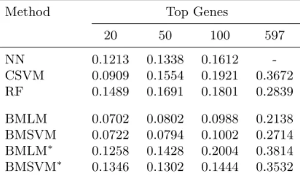
Table 1. Bootstrap error rate of misclassification in the glioma
cancer data. Genes selected by the BW S/BSS criterion.
Method Top Genes
20 50 100 597 NN 0.1213 0.1338 0.1612 -CSVM 0.0909 0.1554 0.1921 0.3672 RF 0.1489 0.1691 0.1801 0.2839 BMLM 0.0702 0.0802 0.0988 0.2138 BMSVM 0.0722 0.0794 0.1002 0.2714 BMLM∗ 0.1258 0.1428 0.2004 0.3814 BMSVM∗ 0.1346 0.1302 0.1444 0.3532
Table 1 reports the total .632 bootstrap estimate of the misclassification error using the formula (7.1). Initially, we used the BW S/BSS criterion as proposed by Dudoit et al. (2002) to order the genes. After we order the genes, we select the top 20, 50, 100 and 597 (i.e., all genes without any selection) genes and use them in the models to predict the class of the “out of bag” sample. The first row indicates the number of top genes included in
the model. As we have pointed out already that the classification of Glioma cancer is extremely difficult, we observe that most of the standard methods like neural network and random forest do equally poorly in classification. With top 20 genes selected by theBW S/BSS criterion, neural network and random forest give bootstrap misclassification errors as 0.1213 and 0.1489 respectively. As we went on adding genes to it, the performance of random forest decayed drastically. With 597 genes, the bootstrap error is nearly the double of what we obtained with top 20 genes. Neural network is much more stable in performance when more genes are added. But again it is impossible to fit a neural network with all the 597 genes. The CSVM worked very well with the top 20 genes, it gave 0.0909 bootstrap error, which is much lower than both the neural network and the random forest. But again, here also by increasing the number of genes to 50 and with any addition thereafter, the performance of the CSVM model diminishes drastically. Our BMLM and BMSVM models (the ones with multiple smoothing parameters) give much better results than all the previous standard models. With the top 20 genes, the bootstrap error is reduced by 20% to 50% in both of our models when compared to the three standard ones. Also, we see that as we increase the number of genes to 100 in our models, their performance is not as affected as the RF, CSVM and NN. But inclusion of all 597 genes gives very high error estimates for all the models, although BMLM and BMSVM continue to improve on CSVM and RF. A main limitation of our BMLM and BMSVM models is that they rely on a two step procedure of gene selection and subsequent class prediction. The main problem in the
BW S/BSS criterion is that we do not know exactly how many top genes we should use, so that we keep on adding more genes in the models.
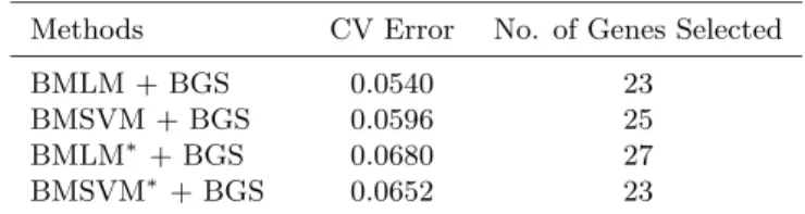
Table 2. Bootstrap error rate of misclassification glioma cancer data. Genes are adaptively selected by the models.
Methods CV Error No. of Genes Selected
BMLM + BGS 0.0540 23
BMSVM + BGS 0.0596 25
BMLM∗+ BGS 0.0680 27
BMSVM∗+ BGS 0.0652 23
In Table 2, we report the results of our models BMLM+BGS and BMSVM +BGS, where we adaptively select the important genes and make the class predictions simultaneously. Both BMLM+BGS and BMSVM+BGS mod-els reduce the bootstrap error by more than 20% than the BMLM and the BMSVM respectively. In BMLM+BGS model, on an average 23 genes are included, and in the BMSVM+BGS, on an average 25 genes are selected.
L06139 M35410 X51602 M92287 M28882 X70326 M34356 M36429 M36430 L05624 L25124 U15172 L29511 M74816 L07414 X90392 M87503 D26156 M97676 M95489 X06256 M64752 M37981 S71824 U60800 Gene Bank Accession ID
BWS/BSS
V00568 L06139 M35410 X51602 M28882 U22398 M25753 L20320 M34356 M36429 M36430 M97675 U34819 U09607 L29511 L07414 X90392 M80627 M95489 A09781 U60800 M36717 M92381 Gene Bank Accession ID
Relative Occurrance (%) in BMLM+BGS
L06139 M35410 X51602 X02751 X92669 X16706 M28882 U22398 M25753 L20320 M28215 M36429 M36430 U34819 M28210 L05624 X68676 L29511 L07414 X90392 M29038 M64752 L06622 S71824 M92381 Gene Bank Accession ID
Relative Occurr ance (%) in BMSVM+BGS 0 1 2 3 4 5 0 2 4 6 8 10 0 2 4 6 8 10
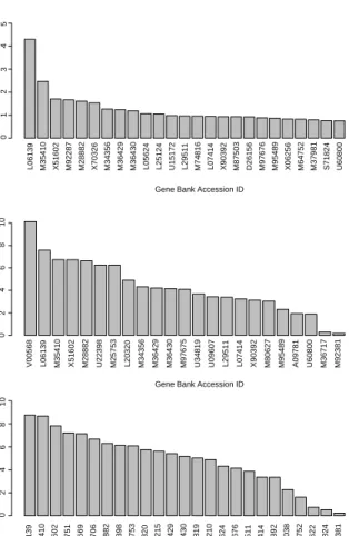
Figure 1. Glioma DNA data. (a) Marginal relevance of Genes by BW S/BSS criterion. (b) Relative number of times a gene is selected by our BMLM+BGS model. (c) Relative number of times a gene is selected by our BMSVM+BGS model.
Figure 1 plots the marginal relevance of each gene by the BW S/BSS
criterion and also the relative number of times each gene appeared in our BMLM+BGS and BMSVM+BGS models. From the figure, we can see that there is an overlap of active genes as suggested by the BW S/BSS criterion and our Bayesian variable selection approach. In fact, there are 8 common important genes selected by both methods. Kim et al. (2002) developed an algorithm for identification of gene sets important for glioma classification. In Table 3, we provide the names of the important genes, which are detected by both of our models and also found to be relevant by the algorithm of Kim et al. (2002). From Table 3, we get that 11 genes are found to match with
Kim’s algorithm, while between the 23 genes selected by BMLM+BGS and the 25 genes selected by BMSVM+BGS, there is a match for 14 such genes. A heat map of the genes selected by our two models and the BWS/BSS criterion is also provided in Figure 2.
Three genes, namely cyclin-dependent kinase inhibitor 1C (CDKN1C), G2/mitotic-specific cyclin B1 (CCNB1) and cell division protein kinase 7 (CDK7), are marked as important by both models but are not selected by Kim’s algorithm or BWS/BSS criterion. In Figure 3, we show the heat map of these three genes, and it appears that they might be important. It is well-known that inducible expression of CDKN1C in cell lines deficient in this cyclin-dependent kinase inhibitor reduces the motility and the invasiveness of malignant gliomas (Sakai et al., 2004). Presence of CCNB1 usually shows an increased growth rate of malignant glioma cell lines and plays a significant role in glioma tumorigenes (Weber et al., 2000). A further investigation may throw more light on the role of these three genes for glioma cancer.
From Tables 1 and 2, we see that we had a significant advantage of using multiple smoothing parameters over single smoothing parameters in terms of bootstrap misclassification error. In all the models with single smoothing parameter, we get higher bootstrap error than the corresponding model with multiple smoothing parameters.
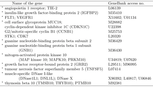
Table 3. Names of the genes selected by both of our models BMLM+BGS and BMSVM+BGS. The genes, which are also identified to be relevant
by the Kim et al. (2002) algorithm, are marked by a ‘∗’.
Name of the gene GeneBank access no.
∗angiopoietin 1 receptor; TIE-2 L06139
∗insulin-like growth factor-binding protein 2 (IGFBP2) M35410
∗FLT1; VEGFR1 X51602; U01134
∗cell surface glycoprotein MUC18; M28882
cyclin-dependent kinase inhibitor 1C (CDKN1C) U22398 G2/mitotic-specific cyclin B1 (CCNB1) M25753
STK1; CDK7 L20320
∗guanine nucleotide-binding protein beta subunit 2 M36429 ∗guanine nucleotide-binding protein beta 1 subunit
(GNB1) M36430
∗mitogen-activated protein kinase 10
(MAP kinase 10; MAPK10; PRKM10) U34819; U07620
∗growth factor receptor-bound protein 2 (GRB2) L29511; M96995 ∗tumour necrosis factor superfamily member 5 (TNFSF5) L07414
∗muscle-specific DNase I-like
(DNase1L1; DNL1L); DNase X X90392; L40817; U06846
Ge n e e x p re ss io n -ba se d g l io ma c l a ss if ic a t io n 53 7 L06139 M35410 X51602 M92287 M28882 X70326 M34356 M36429 M36430 L05624 L25124 U15172 L29511 M74816 L07414 X90392 M87503 D26156 M97676 M95489 X06256 M64752 M37981 S71824 U60800 4 4 4 4 4 3 3 3 3 2 3 3 3 3 2 3 3 2 4 2 2 1 1 1 1 V00568 L06139 M35410 X51602 M28882 U22398 M25753 L20320 M34356 M36429 M36430 M97675 U34819 U09607 L29511 L07414 X90392 M80627 M95489 A09781 U60800 M36717 M92381 4 4 4 4 4 3 3 3 3 2 3 3 3 3 2 3 3 2 4 2 2 1 1 1 1 L06139 M35410 X51602 X02751 X92669 X16706 M28882 U22398 M25753 L20320 M28215 M36429 M36430 U34819 M28210 L05624 X68676 L29511 L07414 X90392 M29038 M64752 L06622 S71824 M92381 4 4 4 4 4 3 3 3 3 2 3 3 3 3 2 3 3 2 4 2 2 1 1 1 1 ur e 2. G lio m a D N A da ta . (a ) H ea tm ap of 25 to p genes sel ect ed b y B W S /B S S er io n. (b) H ea tm ap of 23 to p genes sel ect ed b y our B M L M +B G S m o del . H ea tm ap of 25 to p genes sel ect ed b y our B M SV M +B G S m o del . On the ho ri-ta l ax is on the to p, w e ha ve the G ene B ank A cces sio n N o.
U22398 M25753 L20320 4 4 4 4 4 3 3 3 3 2 3 3 3 3 2 3 3 2 4 2 2 1 1 1 1 Samples
Gene Bank Accession No.
Figure 3. Heatmap of the 3 genes marked as significant by our two models but missed by the Kim’s algorithm and the BWS/BSS criterion.
8 Biological Significance of the Selected Genes in Glioma Cancer
Our BMLM+BGS and BMSVM models have selected 23 genes and 25 genes as relevant respectively based on a marginal posterior probability of 0.01. There is a significant overlap in the gene lists between the two models. In total, 14 genes are found to be common in both the models and are listed in Table 3.
Most of the selected genes carry a lot of biological significance and have putative roles in cancer biology. We focus on potential roles for a few of them. For example, Angiopoietin-2 (Ang2) induces human glioma invasion through the activation of matrix metalloprotease-2 and plays an important role in angiogenesis and tumour progression. Ang2 induces human glioma cell invasion. In invasive areas of primary human glioma specimens, up-regulated expression of Ang2 was detected in tumour cells. Correspondingly higher levels of MMP-2 expression were present in Ang2-expressing tumour cells in these glioma, (Hu et al., 2003).
Another molecule that appears in the list is insulin-like growth factor binding protein 2 (IGFBP2). Wang et al. (2003) showed that IGFBP2 contributes to glioma progression in part by enhancing MMP-2 gene tran-scription and in turn tumour cell invasion.
There is also speculation that progression to glioma requires activation of angiogenesis and has stimulated significant efforts in the development of agents that will block this process. In particular, two pathways have re-ceived considerable attention. They are vascular endothelial growth factor (VEGF) and its receptors, VEGFR1 (Flt-1) and VEGFR2 (Flk-1); note that VEGFR appears on our list of genes in Table 3. VEGF has been shown to be critical for the earliest stages of vasculogenesis, promoting endothelial cell proliferation, differentiation, migration and tubular formation. Gene target-ing studies have shown that deficiency of VEGF, Flt-1 or Flk-1 results in early embryonic lethality caused by defects in angiogenesis and vasculogen-esis (Elizabeth et al., 2001).
Another gene from the list is MUC18, which is a cell adhesion molecule. It has been observed that increased levels of MUC18 results in an increased potential of the cell to grow and divide uncontrollably and thus spreading the glioma (Heimberger et al., 2005). The GNB1 gene included in both of our models is also considered by the biologists as one of the candidate genes for glioma tumour suppressor gene (Collins, 2004).
Some recent experiments support that extracellular signal regulated ki-nase (ERK), a mitogen activated protein kiki-nase, MAPK2 might have a crit-ical role in cell proliferation (Bhaskara et al., 2005). FACS analysis and immunofluorescence studies using monoclonal antibodies, which specifically recognized EGFR, demonstrated that EGFR was expressed predominantly at the cell surface, similar to wild-type (wt) EGFR and to the expression seen in primary biopsy-derived glioma cells (Cavenee, 2002). Phosphotyro-sine residues in the carboxyl tail of wtEGFR provide sites for interaction with SRC homology 2 (SH2) domain-containing adaptor molecules such as SRC and GRB2. Immunoprecipitation studies have shown that EGFR is consti-tutively associated with phosphorylated SHC and GRB2 in several cell lines of different origins. This suggests that the low level constitutive activation of EGFR may cause coupling into unique pathways in these cells and may also point out an entry into interference therapies targeted at gliomas.
The tumour necrosis factor (TNF) superfamily member 5 is also selected by our model. At present, the anti-tumour activity of human recombinant TNF is being examined against various malignant tumours of human origin (Wakabayashi et al., 1997). In the study by Sawada et al. (2004) , they re-ported the anti-tumour activity of recombinant human TNF against human malignant glioma cell lines in vitro and in vivo.
The three genes like CDKN1C, CCNB1 and cell CDK7, which are missed by Kim’s algorithm but captured by us, also carries direct biological signifi-cance in glioma signifi-cancer as mentioned in the previous section.
9 Discussion
Gliomas are very complex cancers involving different growth characteris-tics and cell lineage features (Kleihuse and Cavenee, 2000). As the original clone of tumour cells may exist at any stage of cell differentiation and may have different transformation events, the boundaries between tumour grades and tumour lineages can be blurred. This is reflected in morphologically based tumour classification schemes that often mix cell lineage features with tumour growth characteristics. The results are subjective, and disagreement among pathologists regarding identity of the tumour are very common. The gene expression activities yielded by molecular and genomic biology are more objective to classify diseases as the usual belief is that cell phenotypes have genotypic origins. Recent success in subclassification of neoplasms within a
disease group using gene expression profiles (Golub et al., 1999, Hedenfalk et al., 2001) provide support for such a belief.
The major roadblock is the small sample size issue inherent to micro-array based classification effort. Contributing to this are the limited number of human tissues for study and the cost of such gene expression profiling projects. We want to identify classifiers which: (i) are flexible to execute complex classifications efficiently, (ii) automatically reduce the dimension to accommodate the small sample size problem and (iii) can identify the significant genes. The method based on RKHS developed here satisfies all of these criteria.
The use of RKHS theory helps us to change the dimension of the problem from p to n. In cases when we use the gene expression covariates, p, the number of covariates, is much greater thann, the number of samples. Hence RKHS method provides us with an automatic dimension reduction from p
ton. Earlier papers proposed Bayesian probit model approaches with latent variables for modelling cancer tumours with more than two classes. But all these methods are much restricted compared to ours in the sense that they used simple linear model to model the latent variables. In contrast, our model does not impose any kind of structure on the latent variables. The relationship between the latent variables and the microarray covariates is denoted by an unknown function f. and we assume that the function belongs to an abstract function space, the RKHS. This is the only assumption we make. Then maximize the penalized log likelihood or the posterior to estimate the unknown function. This type of function estimation helps us to come up with a more flexible class of models. Although the use of RKHS helps us to bypass the problem of gene selection by already reducing the dimension of the model from pton, in real life applications, an initial gene selection is always recommended. From Table 1, it is clearly seen that all the standard models and our two models gave extremely poor performance when all genes are used. Rather than doing a two step model fitting, which can induce possible bias in the classifier, i.e, an initial gene selection and then fitting the models using only the selected genes, in Section 6, we suggested an integrated Bayesian gene selection and model fitting approach with the help of indicator variables.
The multicategory SVM proposed by Lee et al. (2004) makes use of the RKHS theory and an extension of the hinge loss. Our BMSVM model is an extension of their approach in the Bayesian paradigm. Lee et al. (2004) treated the whole problem of multiclass classification from an optimization
standpoint, whereas our method treats the whole problem in a probabilis-tic framework. Unlike the frequentist approach, in our method, the kernel parameter θ is not fixed, and we put a prior on it. By putting the prior on the kernel parameter, we gain as we eventually use a mixture of kernels. We can also obtain the full posterior predictive probability distribution of
p(tnew=j), forj = 1, . . . , J, i.e., the probability that a new tumour belongs to thejth type. The full posterior predictive probability distribution con-tains much more information than just a point estimate, and we can easily construct a confidence interval based on it.
The use of near-diffused proper priors helps us to make our method less sensitive to the choice of prior parameters. It also ensures that the posterior is proper so that we can use all standard MCMC techniques to generate samples from it. The procedure is definitely sensitive to the choice ofω as it controls the number of genes each time it is included in the model. In both the examples, we have keptω= 0.01 as suggested by Lee et al. (2004), and Sha et al. (2004). It means that only 10% of the genes are expected to be included in the model, which indirectly implies that we are inducing sparsity. As an alternative, we can also assign a hierarchicalBeta(a, b) prior onω.
Our BMLM and BMSVM have lower misclassification errors than the standard methods like neural network, classical support vector machine and random forest in modelling the glioma cancer. Our methods gave better results than all three standard ones. Both BMLM and BMSVM, when inte-grated with the Bayesian variable selection technique, give improved perfor-mance. Hence we recommend either of our models with multiple smoothing parameters augmented with the Bayesian variable selection technique.
Identifying a particular class or type of glioma cancer is very important for its diagnosis and treatment. Targeting specific therapies to pathogenet-ically distinct tumour types is important for cancer treatment because it maximizes efficacy and minimizes toxicity (Golub et al., 1999). Toxicity plays a major role as the target area of the treatment is the brain or cen-tral nervous system, and any kind of toxic effect of the drug or treatment may lead to long lasting potential hazard to the patient. Diagnostic pathol-ogy has traditionally relied on macro- and microscopic histolpathol-ogy and tumour morphology as the basis for tumour classification. Of all cancers, the gliomas are the hardest to classify and current methods are often unable to do the correct classification. In this paper, our proposed models are able to iden-tify accurately different types of gliomas simultaneously with gene selection.
From Section 8, we see that the genes marked as active or important by our models carry some special biological significance as they can lead to some new lines of investigation for the biologists and geneticists.
In a broader context, the approach applied in this study can be used to identify genes that contribute to the major differences between any two groups of samples analysed. In the process of this, some less understood phe-notypes might be identified. For example, we might find significant genes that distinguish cancers with high metastatic potential from cancers with little or no metastatic potential or genes that identify cancers that will be sensitive to specific therapies versus those that will be resistant and con-tinue to grow unabated through therapy. Current histology-based classifi-cation and grading systems can do neither of these. Identificlassifi-cation of such significant genes may not only provide markers for diagnosis and disease management but may also provide novel potential targets for drug devel-opment. A method that could identify the strong features of cancer, both genotypically and phenotypically, would provide an ideal route to the heart of the problem and we will use our method for these future studies.
References
Albert, J. and Chib, S. (1993). Bayesian analysis of binary and polychotomous
re-sponse data,J. Amer. Statist. Assoc.,88, 669–679.
Allwein, E.L., Schapire, R.E.andSinger, Y.(2000). Reducing multiclass to binary:
a unifying approach for margin classifiers,J. Machine Learning Research, 1, 113– 141.
Alon, U., Barkai, N., Notterman, D.A., Gish, K., Ybarra, S., Mack, D.and
Levine, A.J. (1999). Broad patterns of gene expression revealed by clustering
analysis of tumor and normal colon tissues probed by oligonucleotide arrays. Proc. Natl. Acad. Sci. USA,96, 6745–6750.
Bae, K., Mallick, B.K., Elsik, C.G.(2005). Prediction of protein interdomain linker
regions by a hidden markov model.,Bioinformatics,21, 2264–2270.
Bailey, P.andCushing, H.(1928). A Classification of the Tumors of the Glioma Group
on a Histogenetic Basis with a Correlated Study of Prognosis. J.B. Lippincott, Philadelphia.
Bernardo, J.-M.andSmith, A.F.M.(1994). Bayesian Theory. Wiley Series in
Proba-bility and Mathematical Statistics: ProbaProba-bility and Mathematical Statistics, Wiley, Chichester.
Bhaskara, V.K., Panigrahi, M., Challa, S.andBabu, P.P. (2005). Comparative
status of activated ERK1/2 and PARP cleavage in human gliomas. Neuropathology, 2548.
Braga-Neto, U.M.and Dougherty, E.R.(2004).Is cross-validation valid for
Bredensteiner, E.J.andBennett, K.P.(1999). Multicategory classification by sup-port vector machines. Comput. Optim. Appl.,12, 53–79.
Cairncross, G., Macdonald, D., Ludwin, S., Lee, D., Cascino, T., Buckner,
J., Fulton, D., Dropcho, E., Stewart, D., Schold, C., Wainman, N. and
Eisenhauer, E.(1994). Chemotherapy for anaplastic oligodendroglioma. J.
Clin-ical Oncology,12, 2013–2021.
Cavenee, W.K., (2002). Genetics and new approaches to cancer therapy,
Carcinogene-sis,23, 683–686.
Collins, V.P. (2004). Brain tumours: classification and genes. J. Neurology,
Neuro-surgery and Psychiatry,75, ii2–ii11.
Cover, T.andvan Campenhout, J.(1977). On the possible orderings in the
measure-ment selection problem,IEEE Trans. Systems Man Cybernet.,7, 657–661.
Crammer, K.andSinger, Y.(2001). Ultraconservative online algorithms for multiclass
problems. InComputational Learning Theory(Amsterdam, 2001), D. Helmbold and W. Williamson, eds., Lecture Notes in Computer Science 2111, Springer, Berlin, 99–115.
Denison, D., Holmes, C., Mallick, B.andSmith, A.F.M.(2002). Bayesian Methods
for Nonlinear Classification and Regression. Wiley, London.
DeRisi, J.L., Iyer, V.R.andBrown, P.O.(1997). Exploring the metabolic and genetic
control of gene expression on a genomic scale,Science,278, 680–685.
Dietterich, T.G. and Bakiri, G. (1995). Solving multiclass learning problems via
error-correcting output codes,J. Artificial Intelligence Research,2, 263–286.
Do, K., M¨uller, P., Tang, F.(2004). A nonparametric bayesian mixture model for
gene expression,J. Roy. Statist. Inst., Ser. C,54, 1–18.
Dougherty, E.R.(2001). Small sample issues for microarray-based classification,
Com-parative Functional Genomics,2, 28–34.
Dudoit, S., Fridlyand, J. and Speed, T.P. (2002). Comparison of discrimination
methods for the classification of tumors using gene expression data, J. Amer. Statist. Assoc.,97, 77–87.
Efron, B. (1983). Estimating the error rate of a prediction rule, J. Amer. Statist.
Assoc.,78, 316–333.
Elizabeth et al. (2001)?
Gelfand, A. and Smith, A.F.M. (1990). Sampling-based approaches to calculating
marginal densities,J. Amer. Statist. Assoc.,85, 398–409.
George, E.I.and McCulloch, R. (1993). Variable selection via Gibbs sampling,J.
Amer. Statist. Assoc.,88, 881–889.
Golub, T.R., Slonim, D., Tamayo, P., Huard, C., Gaasenbeek, M., Mesirov,
J., Coller, H., Loh, M., Downing, J., Caligiuri, M., Bloomfield, C. and
Lander, E. (1999). Molecular classification of cancer: class discovery and class
prediction by gene expression monitoring, Science,286, 531–537.
Hastie, T., Tibshirani, R., Eisen, M.B., Alizadeh, A., Levy, R., Staudt, L.,
Chan, W.C., Botstein, D.andBrown, P.O.(2000). Gene shaving as a method
for identifying distinct sets of genes with similar expression patterns, Genome Bi-ology,1, research0003.0001–0003.0021.
Hedenfalk, I., Duggan, D., Chen, Y., Radmacher, M., Bittner, M., Simon, R., Meltzer, P., Gusterson, B., Esteller, M., Kallioniemi, O.P., Wilfond,
B., Borg, A.andTrent, J.(2001). Gene expression profiles in hereditary breast
cancer,New England J. Medicine,344, 539–548.
Heimberger, A.B., McGary, E.C., Suki, D., Ruiz, M., Wang, H., Fuller, G.N.
andBar-Eli, M.(2005). Loss of the AP-2alpha transcription factor is associated
with the grade of human gliomas,Clinical Cancer Research,11, 267–272.
Hu, B., Ping, G., Fang, Q., Tao, H.Q., Wang, D., Nagane, M., Huang, H.S.,
Gunji, Y., Nishikawa, R., Alitalo, K., Cavenee, W.K. and Cheng, S.Y.
(2003). Angiopoietin-2 induces human glioma invasion through the activation of matrix metalloprotease-2,Proc. Natl. Acad. Sci. USA,100, 8904–8909.
Hua, J., Xiong, Z., Lowey, E., Suh, E.andDougherty, E.R.(2005). Optimal
num-ber of features as a function of sample size for various classification rules, Bioinfor-matics,21, 1509–1515.
Hughes, G.F.(1968). On the mean accuracy of statistical pattern recognition, IEEE
Trans. Inform. Theory,14, 55–63.
Ibrahim, J.G., Chen, M.H.andGray, R.J.(2002). Bayesian models for gene
expres-sion with DNA microarray data,J. Amer. Statist. Assoc.,97, 88–99.
Khan, J., Simon, R., Bittner, M., Chen, Y., Leighton, S.B., Pohida, T., Smith,
P.D., Jiang, Y., Gooden, G.C., Trent, J.M.andMeltzer, P.S.(1998). Gene
expression profiling of alveolar rhabdomyosarcoma with cDNA microarrays,Cancer Research,58, 5009–13.
Khan, J., Wei, J.S., Ringn´e r, M., Saal, L.H., Ladanyi, M., Westermann, F.,
Berthold, F., Schwab, M., Antonescu, C.R., Peterson, C.and Meltzer, P.S.
(2001). Classification and diagnostic prediction of cancers using gene expression profiling and artificial neural networks,Nature Medicine,7, 673–679.
Kim, S., Dougherty, E.R., Shmulevich, I., Hess, K.R., Hamilton, S.R., Trent,
J.M., Fuller, G.N. and Zhang W. (2002). Identification of combination gene
sets for glioma classification,Molecular Cancer Therapy,1, 1153–1159.
Kimeldorf, G.andWahba, G.(1971). Some results on Tchebycheffian spline functions,
J. Math. Anal. Appl.,33, 82–95.
Kleihues, P.andCavenee, W.K.(eds.) (2000). Pathology & Genetics of Tumours of
the Nervous System. WHO Series on Pathology & Genetics1, International Agency for Research on Cancer, Lyon, France.
Lee, Y., Lin, Y.andWahba, G.(2004). Multicategory support vector machines, theory,
and application to the classification of microarray data and satellite radiance data,
J. Amer. Statist. Assoc.,99, 67–81.
Lee, K.E., Naijun S., Dougherty, E.R., Vannucci, M.andMallick, B.K.(2003).
Gene selection: a Bayesian variable selection approach,Bioinformatics,19, 90–97.
Mallick, B.K., Ghosh, D.andGhosh, M.(2005). Bayesian classification of tumours
using gene expression data,J. Roy. Statist. Soc. Ser. B,67, 219–232.
Medvedovic M., Sivaganesan S.(2002). Bayesian infinite mixture model based
clus-tering of gene expression profiles,Bioinformatics,18, 1194–1206.
Metropolis, N., Rosenbluth, A.W., Rosenbluth, M.N., Teller, A.H.andTeller,
E.(1953). Equations of state calculations by fast computing machines,J. Chemical Physics,21, 1087–1092.